A robust diagnostic approach for uncertain systems: An example for the jet engine sensor systems

A robust diagnostic approach for uncertain systems: an example for thejet engine sensor systems Pau-Lo

Hsu and Li-Cheng Shen

National Chiao Tung University, Institute of Control Engineering Hsinchu. Taiwan. 300 RO.C.

ABSTRACT

This paper presents a novel eigenstructure assignment approach for synthesizing robust fault detection and isolation (FDI) systems with known inputs. After formulating the FDI problem in eigenstructure assignment, we proceed to develop a parametric characterization of all allowable eigenspaces for disturbance decoupling to achieve robust fault detection. In addition to the structured uncertainties. the robustness of the diagnostic observer to unstructured modeling errors is discussed. A numerical algorithm is further proposed to suppress the effects due to the unstructured uncertainties. The overall robustness of the diagnostic strategy is verified through simulation studies on jet engine systems.

Keyword: fault detection and isolation. unknown inputs, eigenstructure assignment. unstructured uncertainties.

1. DTRODUCTION

The methodology of analytical redundancy is widely employed to economically perform fault detection and isolation (FDI) on controlled systems. The FDI concept based on analytical redundancy uses a mathematical model of the dynamic system to generate the redundancy required to detect malfunctions and isolate faulty components. Methods based on analytical redundancy have been surveyed by Frank,' Gertler,2 and Patton and Chen.3

Approaches based on state observers are now the most favored and important methods of performing FDI. However. limitations regarding accuracy, reliability, and robustness lead to restrictions on the applicability of model-based FDI in practice. Inevitable mismatches between the actual process and its mathematical model frequently render FDI systems unable to tell faults from disturbances. The result is false alarms which adjudge the physical system abnormal even if no fault has occurred and missing alarms when unexpected uncertainties are confused with effects due to faults. Robustness

thus has become a key issue in model-based FDI. The FDI robustness problem has been StUdied by Lou et al..'

Viswanadham and Sridiander,5 Frank Ct al.,6 Patton and Chen.7 and Frank8 In this paper. our interest lies in the problem of structured type of uncertainties in which all uncertainties are summarized as unknown inputs9 with the known distribution matrix acting on the nominal plant.

Eigenstructure assignment has gained special attention because of its flexibility in MIMO control system design, in which the eigenvalues determine the speed of response and the eigenvectors shape the transient espons' Patton and

Chen12 fij

_decoupled structured uncertainties and achieved fault detection by means of eigenstructure assignment. However, the applicability of their method is limited because no complete solution and physical design criterion are provided making it difficult for engineers to implement on physical systems. In a similar way, Watanabe and Himmelblau and Wii nnenberg and Frank proposed an unknown input observer (1.110) to achieve disturbance decoupling, in which the state estimate errors are decoupled from unknown input. Since the solution of an UTO is more complicated than the concept of disturbance decoupling with eigenstructure assignment. and the purpose of a FDI system is to detect fault occurrence instead of state estimate. we prefer the former way to achieve robust FDI design.

In this paper, we propose a robust FDI design based on disturbance decoupling using eigenstructure assignment. Complete solutions through disturbance decoupling with simple matrix computation are provided. In addition to structured uncertainties, the degree of robustness to unstructured type of uncertainties whose characteristics and distribution are unknown is also discussed. Based on time-domain analysis. we obtain robustness measure to bou.nded unstructured uncertainties that helps engineers determine which FDI system best satisfies their requirement. A reduced 5th-order model from a 17th-order jet engine model is presented to demonstrate this approach.

2. ROBUST FAULT DETECTION OBSERVER USING EIGENSTRUCTURE ASSIGNMENT 2.1. Problem statement

Consider the following uncertain system with sensor faults present

x(k+1)= Gx(lc)+Hu(k)+Ed(k)

(1)

y(k)

=

Cx(k)+Du(k)+Kf(k),

(2)

where

x(k) R' is the state vector, u(k) Rm the known input vector, y(k) R the measured signal vector,

d(k) E R formulates the unknown input vector, and f(k) R denotes a fault vector. G, H, C, D, E and K are

known matrices of proper dimensions and r > q. Without loss of generality we may assume that C, E,andK have full rank, and the pair (C, G) is completely observable. The term Kf(k) models the sensor fault effects. The FDI observer is constructed as:

2(k + 1) =(G —

LC)(k)

(H —

_LD)u(k)

+ Ly(k) (3)

5'(k) =C(k)+Du(k)

(4)

r(k) =

W[y(k)—5i(k)], (5)

where r(k) is the residual vector for fault monitoring, L eR is the observer feedback gain matrix, and W ER is a

constant weighting matrix to determine the dimension of residual vector. The corresponding FDI block diagram is

illustratedasinFig. 1.

Input Measurements

u(k) y(k)

r(k) Fig. 1 The block diagram of a FDI observer

To obtain the residual vector dynamics, let e(k) =

_x(k)

—

(k)

_{be the state estimation error. By Eqs. (1-5), we obtain}

e(k±1)=GLe(k)+Ed(k)—LKJ(k)

(6)

r(k) =

WCe(k)+WKJ

(k),

(7)

where GL =(G—

LC).

Therefore, the complete response of the residual vector is

r(z) =

_{Grd(Z)d(Z)+G(Z)f(Z),}

(8) where

Grd(Z)WC(ZJ GL)E

(9)

Grj(z)=WC(zJ

-GL)1 LK+WK = —WIC(zI—

_GL)'

L—_JJK. (10) SPIEVol. 2494 /49 Uncertainties/disturbances Noises Faults

(k)

To achieve robust fault detection, the following conditions must hold true: (i) Grd(Z) =0

_,

whichdecouples disturbances from residual vector r(k)

(ii)[G,- (z)J1 0 and [G,- (1)1 0 ,

wherethe subscript i represent the i-th column of G,-(z). which makes the i-th fault detectable by the residual vector r(z).

Expanding Eq. (9) in eigenstructure. we have

Grd(Z) = WC(flE.

(11)

There are two different ways to make Grd(Z) 0 With eigenstructure assigmnent. One is to choose a W R'"° ffia satisfies WCE = 0 first and, secondly, assign the rows of WC to be the first p left eigenvectors of (G —LC)

.

'fl1j

assignment

givesthatWCv1=Ofori=p+1 nandpE=<WC>1E=Ofori=1,2,...,p,andyieldsthat

Gd(z)=WC

_r

vipT

E=WC

vipT

E=O

z=1 (z—Z) (z—%1)

However, it is seen that the selection of weighting matrix W determines the assignability of eigenvectors. In other words, the rows of WC may be unassignable to the first p left eigenvectors of (G —_LC)even if WCE = 0 .Analternative method is to first determine the last (n —q) left eigenvectors which satisfy pfE = 0 for i = q + 1, .. . ,n from the assignable

eigenspaces of pair (C, G), then, arbitrarily assign the remaining eigenvectors from allowable eigenspaces and determine

w

ER'',

which makes WCv1 = 0 for i = 1,2,...,q .Theunknown inputs are decoupled from the residual vector. In this approach, there is no eigenstructure assignability problem. Therefore, we propose this idea to achieve robust FDI.

2.2. Robust fault detection using the Eigenstructure Assignment Approach

The following Theorem 1 is used to formulate the FDI robustness problem from unknown inputs in eigenstructure. Theorem 1:

Suppose that v and p' are respectively the right and left eigenvectors of GL corresponding to the

eigenvalue .

If

(i) p' E =0 for i = q + 1,... (12) and

(ii)WCv7=Ofori=l,2

q.

(13) then Grd(Z) =0. Proof:

Eq. (9) can be rewritten as

Grd(Z) = wCEl'z1E

[(WCvi)PiWwCE v7(pE)1

1=1 (z—A1) r=q+ (z—A)

It entails that Grd(Z) =0.

I

By Theorem 1, the residual vector is completely decoupled from the unknown inputs so that the robust fault detection is

achieved. Since it is obviously complicated to obtain the assignable eigenvectors fulfilling Eqs. (1243), efficient numerical algorithm for obtaining the allowable eigenvector subspaces is desirable.

2.3. Computation of allowable subspaces: the numerical solution

To systematically develop the numerical procedure for allowable eigenvector subspaces, we introduce a partitioned matrix,

(14)

whose columns constitute the basis of the augmented vector

[:]

(15)

where 1 =1,2,.. .,n

with respect to eigenvalue 2 .

Therefore,

the eigenvector p and the vector

are respectively

parametrized by a column vector a ,i.e.,

p, =

N.

a, and

=

M.

a, . Before computing the allowable subspaces that fulfill Eq. (12-13), we firstly examine the key idea of observer design using the eigenstructure assignment approach by the following Theorem.

Theorem 2.

Consider the nominal system representation R =

_{G,H.C,D}

as in Eqs. (1-2). Suppose that

1= {2 ,22

2, } is a distinct self-conjugate set including the unobservable eigenvalues of the pair (CG) and vectors

p ER" and ERT. If P =

_P2

_{p] being linearly independent and =}

[

•..

_i,,]

_satisfies

[Pi]EN([2J_GT C])fori=1,2....,n.

(16)

then, pT[1J —(G—_LC)1

=0 if L =

pT.T

Proof:

(=)

By Eq. (16), p,T(A,1J —G)-.

'C= 0. Since L =

p_TT

we have that pL =

' for

i =1,2 n. They yield pT[211 —(G— LC)]= 0.

(=)

If pT[211—(G—LCI=o, wehavethat

p(21J—G)—pLC=p(A,J—G)—'C.

or, equivalently, pLC =

'C

for I =1,2,...,n.Since C eRT'"' is full rowrank and r n, it yields that

pTL=fori=1,2

n.

Also, since P is linearly independent, then L =

pTT•

The bases N1 and M can be obtained as follows:

(i)pE=0fori=q+1

Since the assignable eigenvector p1 of the FDI observer with respect to the eigenvalue 2 must satisfy Eq. (16), we have the augmented equation

[21_GT Cnl[pilo

(17)

[

ET

_°iL1J

Sincer > q, Eq. (17) is always solvable so that we obtain the bases N1 and M directly with linear algebra. For arbitraiy

a,, p, =

NA.a1 is assignable in eigenstructu.re assignment.

(ii) WCv1 =0 for 1= 1,...,q:

The bases N and M1 can be directly obtained from the relationship stated in Eq. (16). i.e.. the columns of the partitioned matrix

r1

_,i

-L aJ

constitutethe basis of N([211 —GT

CT]) Arbitrarily choose a, for I =

1.2, ... n to detennine the linearly independent

eigenvector set P =

_[p

_P2 and obtain V =p—T•_{Consequently.}the weighting matrix W is determined by

wI

EN(CV).

(18)

wherewf isthei-throwofWandV1 ={v1 v, •..

_Vq].

Remark 1. If the effect of a fault or the fault itself is soft, the steady-state gain from fault to residual vector has to be scaled by W to avoid missing alarm.

2.4. Summarized numerical algorithm

Step 1. Given R =_{G,H,C. O}, disturbance distribution matrix E. and sensor fault distribution matrix K. Determine the eigenvalue set 1=

,

22

•

.

,

}whichis distinct self-conjugate including the unobservable eigenvalues ofthe pair (C,G).

Step 2. In the case of i =q+ 1, ... n

.

define

S,%1 [GT CT]

(19)

and a compatibly partitioned matrix,

rN2l

ZA [Mj'

(20)

whose coljixnns constitute the bases of N(S,2.).

Step 3. In the case of i =1,2 q ,define

_S,

_[AJ

—_{GT CT] and a compatibly partitioned matrix ., asdefined}

in Eq. (20), whose columns constitute the bases of N(S, ).

Step4. Determine the linear independent eigenvectors p1 =N2.

a1 and

=M2,

a, for I =

1,

2....,n. Obtain the

observer feedback gain L =

p_TT

Step 5. Compute V =

pT

Determine the weighting matrix W from WCV) that meets the specific steady-state gain from faults to residual vector.

3. ROBUSTNESS TO UNSTRUCTURED UNCERTAINTIES

In addition to so-called unknown inputs, another robustness problem arises when uncertainties affecting on system are unstructured for which both characteristics and distribution are unknown. Consider the fault-free and the unknown input-free system in Eqs. (1-2) involving the unstructured uncertainty

x(k + 1) =[G+ AG(x,u))x(k) +[H + MI(x,u)Ju(k) (21)

y(k) =

Cx(k)

+n(k),

(22)

where n(k) represents output noises, and itG(x, u) and EiFI(x,u) formulate the unstructured uncertainty. It is noted that AG(x,u) and LJI(x,u) are non-constant if AG(x,u) and Aff(x, u) are constant, they can be characterized as unknown inputs. The state estimate error and residual dynamics of the diagnostic observer in Eq. (6-7) then becomes

e(k +1)=

_GLe(k)+v(k)

—

_Ln(k)

(23)

r(k) =

WCe(k)+Wn(k). (24)

where v(k) =

_{EG(x,u)x(k) &ff(x,u)u(k)}

. Onecan see that the robust FDI observer of Eqs. (3)(5) is no longer reliable under such circumstances even if the unknown inputs are decoupled. To achieve robust FDI subject to system uncertainties. the observer feedback gain L must be appropriately specified from the allowable solution. Eqs. (2324) lead to the following time response equation for fault-free residuals:

r(k) =

_WC{GLke(O)+

_{GL2ls(k)}+ Wn (k),}

₍₂₅₎

where s(k) =

Ln(k

—i)±v(k —I), e(O) =x(O)—(O) is the initial error condition, and AL =_diag(21

_"2

_2).

_{By taking} the 2-norm ofboth sides ofEq. (25), we obtain the ith residual output (k) as

k

(k)I

=

wTC[GLke(O) + GL1Is(k i)J

+

_wTn(k)

fwfcIf .frALk pTe(O)

+ VAL'' pTs(k ')1

÷

PTII hhhl2 .WTC( .E(k)+JJwTJjn(k)Jl2 =

_K(P)

.JwTCJ . ,(k) + IwT 12 IIn(k)112 (26)

where A(k) =

J1ALc112 .IIe(O)Ij

+JJAL''

₁₂.jjs(k—)ll2 if E.(k) is bounded. K(P) ,_JwfCII and 1w1112 can be treated as

measures of robustness to unstructured uncertainties and measurement noises. i.e.. they should be designed to be as small as possible. Note that to reflect the magnitude of a fault and detect a soft fault, a specific steady state gain is desired. Consequently, K(P), Iwf cli , and are minimized in specific steady-state gain from certain fault to its corresponding residual. To minimize K(P), the eigenvectors must be determined as orthogonal as possible (reference). Unfortunately, the design of Wand P is coupled. By Eq. (10), the steady-state gain from i-th faults to i-th residuals is

—wf[C(J —_GL)' L —_{I]k1, (27)}

where k. is the i-th column of K. It is seen that in a specific DC gain of Eq. (27) the selection of wf is dependent on

[C(J —_GL

) L —

_I]k7and L depends on P. The most orthonormal modal matrix P does not guarantee small ll'T

112. No

optimal solution of Eq. (26) is provided here, while, the solution of wT for minimal 2-norm in specific eigenvectors P is developed by the following Lemma.

Lemma1._{Suppose that N is an orthonormal basis whose columns span the space of w1, then}

(i) if w. lies on the direction =N4 where 5 =

_{N[C(J—Gy'L—Jk7,}

we have minimal 11Wd12

in

constant wTEc(J_GLy1 L—I]kji;

(ii) following (i), if the steady state gain in Eq. (27) is specified as a, then

(28)

112

Proof:

(i) Suppose that w7 liesin the direction i) = Nf37 where/3 is a column vector. It is known that if 8 has minimal angle to b', then Eq. (27) is maximized in all w. N as 11wi112 isconstant. i.e.. we have minimal 11w112 in specific magnitude in

Eq. (27). In other words, the column vector /3;isthe least square solution of

This yields that

then, N/37 =—EC(J—GL)1L—I1kf.

NNWf3j =/

=â,

=

_{NJ7 = N8.}

(29) a.

w.=i1x T

ni a.

= x

5T.{—NEC(J—GL)1L—J]kI} a [—0.9813 I 0.2838 G= —6.8588 1.2235 13.2662 7.5320 —0.5983 0.48575 —0.6979

—0.0826 0.0779 —0.0617 0.0928

—2.2612 0.4141 5.3669 —0.000005 0.00060 1 . C='5x5' andD =05X2. —0.000273 —0.001516 1.6083 —0.3192 —3. 77 10 0.4126 1.0511 —0.0617 —0.1545

E= 1.5659

4.3087 —0.2776 —0. 9646 —2.923 1 —7.8282 (ii) By part (i), we have that

I

4. A DESIGN EXAMPLE: JET ENGINE SYSTEM

To demonstrate the numerical algorithm, a jet engine model are used. The complete system model is originally 17th-order, for practical reasons and convenience of design, Patton and Chen7 approximated the behavior of the engine with a reduced 5th.order model and a disturbance distribution mathx to cover the remaining nonlinearity and modeling error. Consider the following linearized 5th-order discrete time model with 0.026 sec. sampling time

28. 9161 —5.6607 —53.4047 —2.0561 0. 4020 4.7390

0.000139 0.000195

r

0.000067

H= 0.003188

0. 007840 0.003123

The disturbances were summarized in the dominant distribution matrix

and another minor part

0.5334 _{1.1580 i} —0.0768 —0.1644

E'= 1.9658 4.3874 —0.3698 —0.8722

[—3.7068 —8.2010j

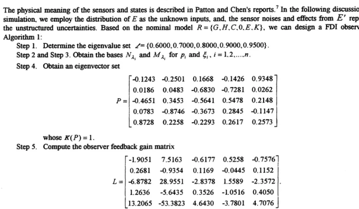
Thephysical meaning of the sensors and states is described in Patton and Chen's reports.7 In the following discussion and

simulation. we employ the distribution of E as the unknown inputs, and, the sensor noises and effects from E'represent the unstructured uncertainties. Based on the nominal model R =

{G,H,C,OEK},

we can design a FDI observer by

Algorithm 1:

Step 1. Determine the eigenvalue set 1 {O. 6000,0.7000,0.8000.0.9000,0.9500). Step 2 and Step 3. Obtain the bases N. and M,. for p7 and

,

i

=1.2

n.

Step4. Obtain an eigenvector set

[-0.1243 -0.2501 0.1668 O.1426 0.9348

0.0186 0.0483 M.6830 -0.7281 0.0262

P=J-0.4651

0.3453 0.564l 0.5478 0.21481 I 0.0783 -0.8746 M.3673 0.2845 -0.1147 L0.8728

0.2258 -0.2293 0.2617 0.2573

whose K(P)= 1.

Step 5. Compute the observer feedback gain matrix

-1.9051 7.5163 -0.6177 0.5258 -0.75761

0.2681

-0.9354 0.1169 -0.0445

0.1152

L= -6.8782 28.9551 -2.8378 1.5589 -2.3572

1.2636 -5.6435 0.3526 -1.0516 0.4050

L 13.2065 -53.3823 4.6430 -3.7801 4.7076]

Arbitrarilychoose weighting matrix w fromthe null space of CV1 such that the steady state gain from the 1st

sensor fault to residual output is 100 as

w=[54.6 —408.6 —152.7 —112.6 —54.8].

5. SIMULATION RESULTS

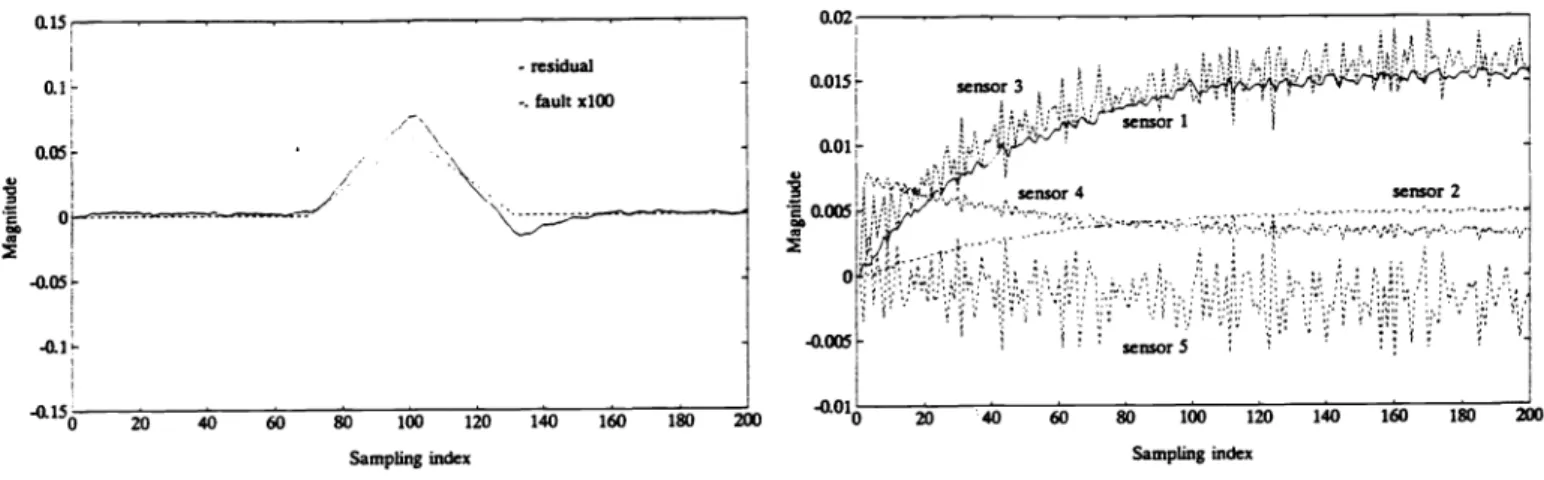
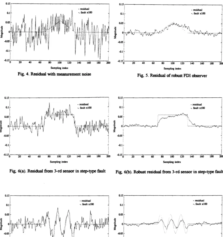
Fig. 2 shows the fault detection result from the first sensor. In this case, sensor noises are not present and a soft fault, whose pick value is 0.000 1, is detected. To observe the detection performance in the presence of measurement noise, we add bounded-random artificial noise with a standard deviation of 0.000 1 at each measurement. Fig. 3 shows the system outputs, and Fig. 4 indicates the detection results under the same operating conditions as those in Fig. 2 except that sensor noise is included. It can be seen that the detection perfonnance degrades in the presence of noise. According to the discussion in Sec. 3 on robustness to unstructured uncertainties, we apply Lemma 1 to determine an alternative weighting

matrix

w=[35.4426

16.3019

-30.4057 -23.6654 -9.3822].

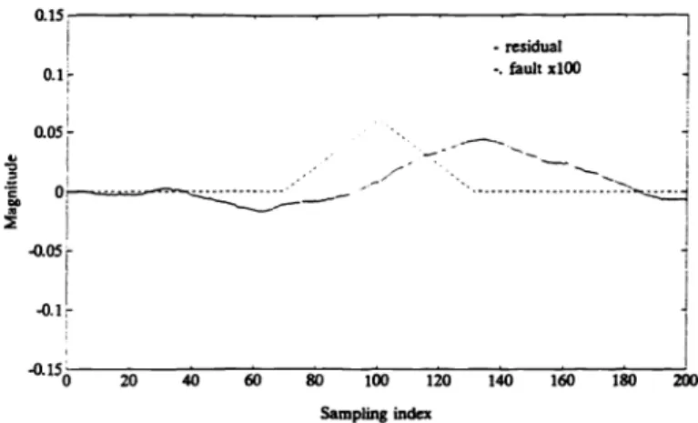
The corresponding diagnostic result is shown in Fig. 5. Clearly, the effects of noise on residual are suppressed without loss of detectionability. To verify our work, diagnostic results from the third sensor in the jet engine system are demonstrated in Figs. 6 and 7, with step-type and sinusoidal-type faults, respectively. Fig. 6(a) and Fig. 7(a) show the results in which the weighting matrix W is arbitrarily chosen to be

w=[—2L8 163.4 61.0 45.0 21.9],

and Fig. 6(b) and Fig. 7(b) are the diagnostic results of a robust weighting design by Lemma 1:

w

=_[0.4662 -7.9472 22.73 18 1 1.3300 11.3350].

Apparently,the proposed robust FDI design significantly improves the diagnostic performance when system uncertainty is

present. The simulation results in Figs. 6 and 7 provide a direct verification of our work.

Remark 2. Most published papers about eigenstructure assignment claim that the eigenvectors should be chosen as mutually orthogonal as possible to obtain a well-conditioned modal matrix. While, in Sec. 3. the robustness of detection performance to unstructured uncertainties is found to be dependent on the weighting matrix W and K(P) from which the effects are coupled. In other words, well-conditioned eigenvector assignment may result in high 2-norm of W. The conditioning ofthe observer modal matrix should be properly determined. Take the case in Fig. 3 above as an example, the eigenvectors are alternatively chosen as

-0.1226 0.2510 0.6294 0.4671 -0.46451

0.0183 0.0484 0.7040 0.0824 0.0790

P= -0.4674 0.3422 -0.2267 -0.7231 -0.7245

0.0841 -0.8740 -0.2371 -0.2585 -0.2601

0.8712 0.2316 -0.0250 -0.4305 -0.4307

whosecondition number is about 421. Consequently, the output feedback gain matrix 0.8892 7.1113

3.6208 2.0311

1.7732 -3.1170 -0.3467 -5.3067 -2.0136 -3.0935

L= -8.3418 29.1509 -5.1531 0.7197 -3.7288 1 -0.3431 -5.4144 -2.1485 -1.9504 -L0804 I 13.0411 -53.3688 4.3527 -3.8896 4.5386 j

isobtained and the W determined by Lemma 1 is

W=[0.2192 -0.2777 -0.1204 -0.1295 -0.0154].

The diagnostic result is shown in Fig. 8. It is seen that the noise rejection is improved but the detection time gets slower. Readers should note the trade-offbetween detection time and robustness to measurement noise.

6. CONCLUSION

In this paper, we proposed a FDI observer robust to unknown inputs through disturbance decoupling with

eigenstructure assignment. Other than the concept of disturbance decoupling proposed by Patton and Chen, we formulate the robustness problem starting from allowable eigenspaces decoupling unknown inputs so that the desired eigenstructure is always assignable. Our numerical treatment provides complete solutions for allowable FDI which decouples unknown inputs from failures. In addition to structured uncertainties, unstructured uncertainties, for which neither characteristics nor distribution are known in advance, were addressed in this paper since a physical system can not be completely described by analytical models. In our simulation results, the presence of measurement noise and modeling errors brought up the problem of robustness, even though the unknown inputs were decoupled. Also, the weighting matrix and the condition number of eigenvectors were treated as two important indices of the FDI system's robustness to unstructured uncertainties. In real applications, it would be more appropriate to use eigenvector assigiunent to decouple the dominant unknown inputs and then suppress theeffectsof unstructured uncertainties by_minimizingthetotalquantity of K(P) and _ll2

7. REFERENCES

1. P. M. Frank, "Fault Diagnosis in Dynamic Systems Using Analytical and Knowledge-Based Redundancy -

A

Survey and Some New Results," Automatica,Vol._{26, pp. 459-474, 1990.}

2. J. Gertler, "Residual Generation in Model-Based Fault Diagnosis," Control-Theory and Advanced Technology, Vol. 9, No. 1, pp.259-285,1993.

3. R. J. Patton and 3. Chen, "Review of Parity Space Approaches to Fault Diagnosis for Aerospace Systems" AJAA

JournalofGuidance, Control, andDynamics. Vol. 17, pp. 278-285. 1994.

4. X. C. Lou. A. S. Wilisky. and. G. L. Verghese. "Optimally Robust Redundancy Relations for Failure Detection in Uncertain System," Automatica, Vol. 22, pp. 333.334. 1986

5. N. Viswanadham and R. Srichander. "Fault Detection Using Unknown Input Observers," Control Theory and Advanced Technology, Vol. 3. No. 2, pp. 91-101, 1 987.

6. P. M. Frank, B. Koeppen. and, J. Wil nnenberg, "General Solution of Robustness Problem in Linear-Fault

Detection Filters," First European Control Conference ECC 91, pp. 1407-1412, 1991.

7. R. J. Patton and J. Chen, "Robust Fault Detection of Jet Engine Sensor Systems Using Eigenstructure

Assignment," Journal ofGuidance. Control, andDynamics. Vol. 15. No. 6. pp. 1491-1497. 1992.

8. P. M. Frank, "Enhancement of Robustness in Observer-Based Fault Detection," mt. J.Control, Vol. 59. pp. 955-981, 1994.

9. R. J. Patton and J. Chen._"Optimal Unknown Input Distribution Mathx Selection in RObUSt Fault Diagnosis,"

Automatica,Vol.29, No. 4, pp. 1491-1497. 1993.

10. B. C. Moore, "On the Flexibility Offered by State Feedback in Multivariable Systems Beyond Closed Loop

EigenvalueAssignment,"IEEE Trans. Automatic Control, Vol. AC-21, pp. 689-692. 1976.

11. A. N. Andry, J. C. Chung, and E. Y. Shapiro, "Modalized Observer." IEEE Trans. Automatic Control, Vol.

AC-29,pp. 669-672, 1984.

12. R. J.Pattonand_{J. Chen,}"RobustFaultDetection UsingEigenstructure Assignment: A Tutorial Consideration and

Some New Result," Proc. of the 30th Conf on Detection and Control, pp. 2242-2247. Brighton, England, 1991.

residual 0.1-..faultxlOO 0.05[ .

/

.05L .o.iL -0.15 io so 6o 80 100 12 140 160 180 200 Sampling index

Fig.3. Measurementwith disturbance and noise

SPIEVol. 2494 /57

Sampling index

Fig.2. Residualwithout measurement noise

sensor 2

sensor 4

' '-- - -"--- --- - -. -.

00

Sampling index

Fig. 5.Residualof robust FDI observer

00

00

Sampling index

Fig. 6(a). Residual from 3-rd sensor in step-type fault

- residual

fault xlOO

jr-•u•L0 20 40 60 80 100 120 140 160 180 200

Sampling index

Fig. 6(b). Robust residual from 3-rd sensor in step-type fault

Fig. 7(a). Residual from 3-rd sensor in sin.-type fault

58/ SPIE Vol. 2494

Fig. 7(b). Robust residual from 3-rd sensor in sin-type fault

- residual

-.faultxlOO

Sampling index

Fig. 4. Residual with measurement noise

-.--0 20 40 60 80 100 120 140 - 160 180 200 - residual -. faultxlOO Sampling index

'0 20

40 60 80 100 120 140 160 180 200 Sampling index

- residual

O.lr -.fault xlOO

°•°5r

oH

-O.O5-•vlSÔ

o

80 100 120 140 160 180 200 Sampling index

Fig. 8. Residual output with ill-conditioned eigenvector deisgn