SVM-RFE Based Feature Selection and Taguchi Parameters Optimization for Multiclass SVM Classifier

(1)

Research Article

SVM-RFE Based Feature Selection and Taguchi Parameters

Optimization for Multiclass SVM Classifier

Mei-Ling Huang,

1

Yung-Hsiang Hung,

1

W. M. Lee,

2

R. K. Li,

2

and Bo-Ru Jiang

1

1_{Department of Industrial Engineering and Management, National Chin-Yi University of Technology, No. 57, Sec. 2,}

Zhong-Shan Road, Taiping District, Taichung 41170, Taiwan

2_{Department of Industrial Engineering & Management, National Chiao-Tung University, No. 1001, Ta-Hsueh Road,}

Hsinchu 300, Taiwan

Correspondence should be addressed to Mei-Ling Huang; [email protected]

Received 20 June 2014; Revised 5 August 2014; Accepted 5 August 2014; Published 10 September 2014 Academic Editor: Shifei Ding

Copyright © 2014 Mei-Ling Huang et al. This is an open access article distributed under the Creative Commons Attribution License, which permits unrestricted use, distribution, and reproduction in any medium, provided the original work is properly cited.

Recently, support vector machine (SVM) has excellent performance on classification and prediction and is widely used on disease diagnosis or medical assistance. However, SVM only functions well on two-group classification problems. This study combines feature selection and SVM recursive feature elimination (SVM-RFE) to investigate the classification accuracy of multiclass problems for Dermatology and Zoo databases. Dermatology dataset contains 33 feature variables, 1 class variable, and 366 testing instances; and the Zoo dataset contains 16 feature variables, 1 class variable, and 101 testing instances. The feature variables in the two datasets were sorted in descending order by explanatory power, and different feature sets were selected by SVM-RFE to explore classification accuracy. Meanwhile, Taguchi method was jointly combined with SVM classifier in order to optimize parameters𝐶 and 𝛾 to increase classification accuracy for multiclass classification. The experimental results show that the classification accuracy can be more than 95% after SVM-RFE feature selection and Taguchi parameter optimization for Dermatology and Zoo databases.

1. Introduction

The support vector machine (SVM) is one of the important tools of machine learning. The principle of SVM operation is as follows: a given group of classified data is trained by the algorithm to obtain a group of classification models, which can help predict the category of the new data [1, 2]. Its scope of application is widely used in various fields, such as disease or medical imaging diagnosis [3–5], financial crisis prediction [6], biomedical engineering, and bioinformatics classification [7,8]. Although SVM is an efficient machine learning method, its classification accuracy requires further improvement in the case of multidimensional space clas-sification and dataset for feature interaction variables [9]. Regarding such problems, in general, feature selection can be applied to reduce data structure complexity in order to identify important feature variables as a new set of testing instances [10]. By feature selection, inappropriate, redundant, and noise data of each problem can be filtered to reduce

the computational time of classification and improve classi-fication accuracy. The common methods of feature selection include backward feature selection (BFS), forward feature selection (FFS), and ranker [11]. Another feature selection method, support vector machine recursive feature elimina-tion (SVM-RFE), can filter relevant features and remove relatively insignificant feature variables in order to achieve higher classification performance [12]. The research findings of Harikrishna et al. have shown that computation is simpler and can more effectively improve classification accuracy in the case of datasets after SVM-REF selection [13–15].

As SVM basically applies on two-class data [16], many scholars have explored the expansion of SVM on multiclass data [17–19]. However, classification accuracy is not ideal. There are many studies on choosing kernel parameters for SVM [20–22]. Therefore, this study applies SVM-RFE to sort the 33 variables for Dermatology dataset and 16 variables for Zoo dataset by explanatory power in descending order and selects different feature sets before using the Taguchi

Volume 2014, Article ID 795624, 10 pages http://dx.doi.org/10.1155/2014/795624

(2)

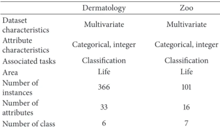
Table 1: Feature information for Dermatology and Zoo databases.

Dermatology Zoo

Dataset

characteristics Multivariate Multivariate Attribute

characteristics Categorical, integer Categorical, integer Associated tasks Classification Classification

Area Life Life

Number of

instances 366 101

Number of

attributes 33 16

Number of class 6 7

parameter design to optimize Multiclass SVM parameters𝐶 and𝛾 to improve the classification accuracy for SVM multi-class multi-classifier.

This study is organized as follows.Section 2describes the research data; Section 3 introduces methods used through this paper; Section 4discusses the experiment and results. Finally,Section 5presents our conclusions.

2. Study Population

This study used the Dermatology dataset from University of California at Irvine (UCI) and the Zoo database from its College of Information Technology and Computers to conduct experimental tests, parameter optimization, and classification accuracy performance evaluation, using the SVM classifier.

In medicine, dermatological diseases are diseases of the skin that have a serious impact on health. As frequently occurring types of diseases, there are more than 1000 kinds of dermatological diseases, such as psoriasis, seborrheic dermatitis, lichen planus, pityriasis, chronic dermatitis, and pityriasis rubra pilaris. The Dermatology dataset was estab-lished by Nilsel in 1998 and contains 33 feature variables and 1 class variable (6-class).

The dermatology feature variables and data summary are as shown inTable 1. The Dermatology dataset has eight omissions. After removing the eight omissions, we retained 358 (instances) for this study. The instances of data of various categories are psoriasis (Class 1): 111 instances, seborrheic dermatitis (Class 2): 71 instances, lichen planus (Class 3): 60 instances, pityriasis (Class 4): 48 instances, chronic dermatitis (Class 5): 48 instances, and pityriasis rubra pilaris (Class 6): 20 instances. The Zoo dataset contains 17 Boolean-valued attributes and 101 instances. The instances of data of various categories are as follows: bear, and so forth (Class 1) 41 instances; chicken, and so forth (Class 2) 20 instances; seasnake, and so forth (Class 3) 5 instances; bass, and so forth (Class 4) 13 instances; (Class 5) 4 instances; frog, and so forth (Class 6) 8 instances; and honeybee, and so forth (Class 7) 10 instances.

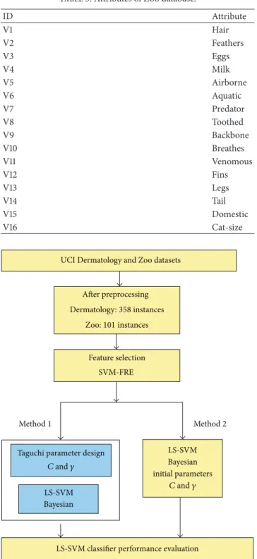
Before feature selection, we conducted feature attribute coding. The feature attribute coding of Dermatology and Zoo databases is as shown in Tables2and3.

Table 2: Attributes of Dermatology database.

ID Attribute V1 Erythema V2 Scaling V3 Definite borders V4 Itching V5 Koebner phenomenon V6 Polygonal papules V7 Follicular papules

V8 Oral mucosal involvement

V9 Knee and elbow involvement

V10 Scalp involvement

V11 Family history

V12 Melanin incontinence

V13 Eosinophils in the infiltrate

V14 PNL infiltrate

V15 Fibrosis of the papillary dermis

V16 Exocytosis

V17 Acanthosis

V18 Hyperkeratosis

V19 Parakeratosis

V20 Clubbing of the rete ridges V21 Elongation of the rete ridges

V22 Thinning of the suprapapillary epidermis

V23 Spongiform pustule

V24 Munro microabscess

V25 Focal hypergranulosis

V26 Disappearance of the granular layer V27 Vacuolisation and damage of basal layer

V28 Spongiosis

V29 Saw-tooth appearance of retes

V30 Follicular horn plug

V31 Perifollicular parakeratosis

V32 Inflammatory mononuclear infiltrate

V33 Band-like infiltrate

V34 Age

3. Methodology

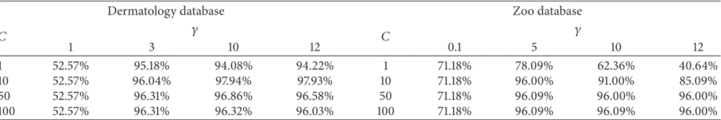
3.1. Research Framework. The research framework of the

study is shown inFigure 1. Steps are as follows.

(1) Database preprocessing: delete the omissions and feature variable coding for Dermatology and Zoo datasets. And there are 358 and 101 instances left for Dermatology and Zoo databases for further experi-ment, respectively.

(2) Feature selection: apply SVM-RFE ranking according to the order of importance of the features, and determine the feature set that contributes to the classification.

(3) Parameter optimization: apply Taguchi parameter design in the parameters (𝐶 & 𝛾) optimization of a Multiclass SVM Classifier in order to enhance the classification accuracy for the multiclass dataset.

(3)

Table 3: Attributes of Zoo database. ID Attribute V1 Hair V2 Feathers V3 Eggs V4 Milk V5 Airborne V6 Aquatic V7 Predator V8 Toothed V9 Backbone V10 Breathes V11 Venomous V12 Fins V13 Legs V14 Tail V15 Domestic V16 Cat-size

UCI Dermatology and Zoo datasets

After preprocessing Dermatology:358 instances Zoo:101 instances Feature selection SVM-FRE Method1 Method2

Taguchi parameter design C and 𝛾 LS-SVM Bayesian LS-SVM Bayesian initial parameters C and 𝛾

LS-SVM classifier performance evaluation

Figure 1: Research framework.

3.2. Feature Selection. Feature selection implies not only

cardinality reduction, which means imposing an arbitrary or predefined cutoff on the number of attributes that can be considered when building a model, but also the choice of attributes, meaning that either the analyst or the modeling tool actively selects or discards attributes based on their usefulness for analysis. The feature selection method is a search strategy to select or remove some features of the

original feature set to generate various types of subsets to obtain the optimum feature subset. The subsets selected each time are compared and analyzed according to the formulated assessment function. If the subset selected in step𝑚 + 1 is better than the subset selected in step𝑚, the subset selected in step𝑚 + 1 can be selected as the optimum subset.

3.3. Linear Support Vector Machine (Linear SVM). SVM is

developed from statistical learning theory, as based on SRM (structural risk minimization). It can be applied on classifica-tion and nonlinear regression [6]. Generally speaking, SVM can be divided into linear SVM (linear SVM) and nonlinear SVM, described as follows.

(1) Linear SVM. The linear SVM encodes the training data

of different types by classification with Class 1 as being “+1” and Class 2 as being “−1” and the mathematical symbol is {{𝑥_𝑖, 𝑦_𝑖}𝑇_𝑖−1, 𝑥_𝑖 ∈ R𝑚, 𝑦_𝑖 ∈ {−1, +1}}; the hyperplane is represented as follows:

𝑤 ⋅ 𝑥 + 𝑏 = 0, (1)

where𝑤 denotes weight vector, 𝑥 denotes the input dataset, and 𝑏 denotes a constant as a bias (displacement) in the hyperplane. The purpose of bias is to ensure that the hyper-plane is in the correct position after horizontal movement. Therefore, bias is determined after training𝑤. The parameters of the hyperplane include𝑤 and 𝑏. When SVM is applied on classification, the hyperplane is regarded as a decision function:

𝑓 (𝑥) = sign (𝑤 ⋅ 𝑥 + 𝑏) . (2)

Generally speaking, the purpose of SVM is to obtain the hyperplane of the maximized marginal distance and improve the distinguishing function between the two categories of the dataset. The process of optimizing the distinguishing function of the hyperplane can be regarded as a quadratic programming problem:

minimize 𝐿_𝑝= 1 2‖𝑤‖2

subject to 𝑦_𝑖(𝑥_𝑖⋅ 𝑤 + 𝑏) − 1 ≥ 0, 𝑖 = 1, . . . , 𝑙. (3)

The original minimization problem is converted into a maximization problem by using the Lagrange Theory:

max 𝐿_𝐷(𝛼) = 𝑙 ∑ 𝑖=1 𝛼_𝑖−1 2 𝑙 ∑ 𝑖=1 𝑙 ∑ 𝑗=1 𝛼_𝑖𝛼_𝑗𝑦_𝑖𝑦_𝑗(𝑥_𝑖𝑥_𝑗) subject to 𝑙 ∑ 𝑖=1 𝛼_𝑖𝑦_𝑖= 0, 𝑖 = 1, . . . , 𝑙 𝛼𝑖≥ 0, 𝑖 = 1, . . . , 𝑙. (4)

Finally, the linear divisive decision making function is 𝑓 (𝑥) = sign (∑𝑛

𝑖=1

(4)

If𝑓(𝑥) > 0, it means the sample is in the same category as samples marked with “+1”; otherwise, it is in the category of samples marked with “−1.” When the training data include noise, the linear hyperplane cannot accurately distinguish data points. By introducing slack variables𝜉_𝑖in the constraint, the original (3) can be modified into the following:

minimize 1 2‖𝑤‖2+ 𝐶 ( 𝑙 ∑ 𝑖=1 𝜉_𝑖) subject to 𝑦_𝑖(𝑥_𝑖⋅ 𝑤 + 𝑏) − 1 + 𝜉_𝑖≥ 0, 𝑖 = 1, . . . , 𝑙 𝜉_𝑖≥ 0, 𝑖 = 1, . . . , 𝑙, (6)

where𝜉_𝑖is the distance between the boundary and the clas-sification point and penalty parameter𝐶 represents the cost of the classification error of training data during the learning process, as determined by the user. When𝐶 is greater, the margin will be smaller, indicating that the fault tolerance rate will be smaller when a fault occurs. Otherwise, when 𝐶 is smaller, the fault tolerance rate will be greater. When 𝐶 → ∞, the linear inseparable problem will degenerate into a linear separable problem. In this case, the solution of the above mentioned optimization problem can be applied to obtain the various parameters and optimum solution of the target function using the Lagrangian coefficient; thus, the linear inseparable dual optimization problem is as follows:

Max 𝐿_𝐷(𝛼) = 𝑙 ∑ 𝑖=1 𝛼_𝑖−1₂∑𝑙 𝑖=1 𝑙 ∑ 𝑗=1 𝛼_𝑖𝛼_𝑗𝑦_𝑖𝑦_𝑗(𝑥_𝑖𝑥_𝑗) Subject to 𝑙 ∑ 𝑖=1 𝛼_𝑖𝑦_𝑖= 0, 𝑖 = 1, . . . , 𝑙 0 ≤ 𝛼_𝑖≤ 𝐶, 𝑖 = 1, . . . , 𝑙. (7)

Finally, the linear decision-making function is 𝑓 (𝑥) = sign (∑𝑛

𝑖=1

𝑦_𝑖𝛼∗_𝑖 (𝑥 ⋅ 𝑥_𝑖) + 𝑏∗) . (8)

(2) Nonlinear Support Vector Machine (Nonlinear SVM).

When input training samples cannot be separated using linear SVM, we can use conversion function 𝜑 to convert the original 2-dimensional data into a new high-dimensional feature space for linear separable problem. SVM can effi-ciently perform a nonlinear classification using what is called the kernel trick, implicitly mapping their inputs into high-dimensional feature spaces. Presently, many different core functions have been proposed. Using different core functions regarding different data features can effectively improve the computational efficiency of SVM. The relatively common core functions include the following four types:

(1) linear kernel function:

𝐾 (𝑥_𝑖, 𝑦_𝑖) = 𝑥𝑡_𝑖⋅ 𝑦_𝑗, (9)

(2) polynomial kernel function:

𝐾 (𝑥_𝑖, 𝑦_𝑗) = (𝛾𝑥𝑡_𝑖𝑥_𝑗+ 𝑟)𝑚, 𝛾 > 0, (10) (3) radial basis kernel function:

𝐾 (𝑥_𝑖, 𝑦_𝑗) = exp (−󵄩󵄩󵄩󵄩󵄩𝑥𝑖− 𝑦𝑗󵄩󵄩󵄩󵄩󵄩

2

2𝜎2 ) , 𝛾 > 0, (11)

(4) sigmoid kernel function:

𝐾 (𝑥_𝑖, 𝑦_𝑗) = tanh (𝛾𝑥𝑡_𝑖⋅ 𝑦_𝑗+ 𝑟) , (12) where the emissive core function is more frequently applied in high feature dimensional and nonlinear problems, and the parameters to be set are 𝛾 and 𝐶, which can slightly reduce SVM complexity and improve calculation efficiency; therefore, this study selects the emissive core function.

3.4. Support Vector Machine Recursive Feature Elimination (SVM-RFE). A feature selection process can be used to

remove terms in the training dataset that are statistically uncorrelated with the class labels, thus improving both efficiency and accuracy. Pal and Maiti (2010) provided a supervised dimensionality reduction method. The feature selection problem has been modeled as a mixed 0-1 inte-ger program [23]. Multiclass Mahalanobis-Taguchi system (MMTS) is developed for simultaneous multiclass classi-fication and feature selection. The important features are identified using the orthogonal arrays and the signal-to-noise ratio and are then used to construct a reduced model measurement scale [24]. SVM-RFE is an SVM-based feature selection algorithm created by [12]. Using SVM-RFE, Guyon et al. selected key and important feature sets. In addition to reducing classification computational time, it can improve the classification accuracy rate [12]. In recent years, many schol-ars improved the classification effect in medical diagnosis by taking advantage of this method [22,25].

3.5. Multiclass SVM Classifier. SVM’s basic classification

principle is mainly based on dual categories. Presently, there are three main methods, one-against-all, one-against-one, and directed acyclic graph, to process multiclass problems [26], described as follows.

(1) One-Against-All (OAA). Proposed by Bottou et al., (1994)

the one-versus-rest converts the classification problem of𝑘 categories into𝑘 dual-category problems [27]. Scholars have also proposed subsequent effective classification methods [28]. In the training process, it must train𝑘 dual-category SVMs. When training the 𝑖th classifier, data in the 𝑖th category is regarded as “+1” and the data of the remaining categories is regarded as “−1” to complete the training of 𝑘 dual-category SVM; during the testing process, each testing instance is tested by trained𝑘 dual-category SVMs. The classification results can be determined by comparing the outputs of SVM. Regarding unknown category 𝑥, the

(5)

decision function arg max_{𝑖=1,...,𝑘}(𝑤𝑖)𝑡𝜙(𝑥) + 𝑏𝑖can be applied to generate𝑘 decision-making values, and category 𝑥 is the category of the maximum decision making value.

(2) One-Against-One (OAO). When there are𝑘 categories,

two categories can produce an SVM; thus, it can produce𝑘(𝑘− 1)/2 classifiers and determine the category of the samples by a voting strategy [28]. For example, if there are three categories (1, 2, and 3) and a sample to be classified with an assumed category of 2, the sample will then be input into three SVMs. Each SVM will determine the category of the sample using decision making function sign((𝑤𝑖𝑗₎𝑡_{Φ(𝑥) + 𝑏}𝑖𝑗_{) and adds 1 to}

the votes of the category. Finally, the category with the most votes is the category of the sample.

(3) Directed Acyclic Graph (DAG). Similar to OAO method,

DAG is to disintegrate the classification problem𝑘 categories into a𝑘(𝑘 − 1)/2 dual-category classification problem [18]. During the training process, it selects any two categories from𝑘 categories as a group, which it combines into a dual-category classification SVM; during the testing process, it establishes a dual-category acyclic graph. The data of an unknown category is tested from the root nodes. In a problem with𝑘 classes, a rooted binary DAG has 𝑘 leaves labeled by the classes where each of the𝑘(𝑘 − 1)/2 internal nodes is labeled with an element of a Boolean function [19].

4. Experiment and Results

4.1. Feature Selection Based on SVM-RFE. The main purpose

of SVM-RFE is to compute the ranking weights for all features and sort the features according to weight vectors as the classification basis. SVM-RFE is an iteration process of the backward removal of features. Its steps for feature set selection are shown as follows.

(1) Use the current dataset to train the classifier. (2) Compute the ranking weights for all features. (3) Delete the feature with the smallest weight.

Implement the iteration process until there is only one feature remaining in the dataset; the implementation result provides a list of features in the order of weight. The algorithm will remove the feature with smallest ranking weight, while retaining the feature variables of significant impact. Finally, the feature variables will be listed in the descending order of explanatory difference degree. SVM-RFE’s selection of feature sets can be mainly divided into three steps, namely, (1) the input of the datasets to be classified, (2) calculation of weight of each feature, and(3) the deletion of the feature of minimum weight to obtain the ranking of features. The computational step is shown as follows [12].

(1) Input

Training sample:𝑋₀= [𝑥₁, 𝑥₂, . . . , 𝑥_𝑚]𝑇. Category:𝑦 = [𝑦₁, 𝑦₂, . . . , 𝑦_𝑚]𝑇.

The current feature set:𝑠 = [1, 2, . . . , 𝑛]. Feature sorted list:𝑟 = [].

(2) Feature Sorting

Repeat the following process until𝑠 = [].

To obtain the new training sample matrix according to the remaining features:𝑋 = 𝑋₀(:, 𝑠).

Training classifier:𝛼 = SVM-train(𝑋, 𝑦). Calculation of weight:𝑤 = ∑_𝑘𝛼_𝑘𝑦_𝑘𝑥_𝑘. Calculation of sorting standards:𝑐_𝑖= (𝑤_𝑖)2.

Finding the features of the minimum weight: 𝑓 = arg min(𝑐).

Updating feature sorted list:𝑟 = [𝑠(𝑓), 𝑟].

Removing the features with minimum weight:𝑠 = 𝑠(1 : −1, 𝑓 + 1 : length(𝑠)).

(3) Output: Feature Sorted List𝑟. In each loop, the feature

with minimum(𝑤_𝑖)2will be removed. The SVM then retrains the remaining features to obtain the new feature sorting. SVM-RFE repeatedly implements the process until obtaining a feature sorted list. Through training SVM using the feature subsets of the sorted list and evaluating the subsets using the SVM prediction accuracy, we can obtain the optimum feature subsets.

4.2. SVM Parameters Optimization Based on Taguchi Method.

Taguchi Method rises from the engineering technological perspective and its major tools include the orthogonal array and𝑆𝑁 ratio, where 𝑆𝑁 ratio and loss function are closely related. A higher𝑆𝑁 ratio indicates fewer losses [29]. Param-eter selection is an important step of the construction of the classification model using SVM. The differences in parameter settings can affect classification model stability and accuracy. Hsu and Yu (2012) combined Taguchi method and Staelin method to optimize the SVM-based e-mail spam filtering model and promote spam filtering accuracy [30]. Taguchi parameter design has many advantages. For one, the effect of robustness on quality is great. Robustness reduces variation in parts by reducing the effects of uncontrollable variation. More consistent parts are equal to better quality. Also, the Taguchi method allows for the analysis of many different parameters without a prohibitively high amount of experimentation. It provides the design engineer with a systematic and efficient method for determining near optimum design parameters for performance and cost. Therefore, by using the Taguchi qual-ity parameter design, this study conducts the optimization design of parameters𝐶 and 𝛾 to enhance the accuracy of SVM classifier on the diagnosis of multiclass diseases.

This study uses the multiclass classification accuracy as the quality attribute of the Taguchi parameter design [21]. In general, when the classification accuracy is higher, it means the accuracy of the classification model is better; that is, the quality attribute is larger-the-better (LTB), and𝑆𝑁LTBis

defined as: 𝑆𝑁LTB= −10 log₁₀(𝑀𝑆𝐷) = −10 log₁₀[ 1 𝑛 𝑛 ∑ 𝑖=1 1 𝑦2 𝑖 ] . (13)

(6)

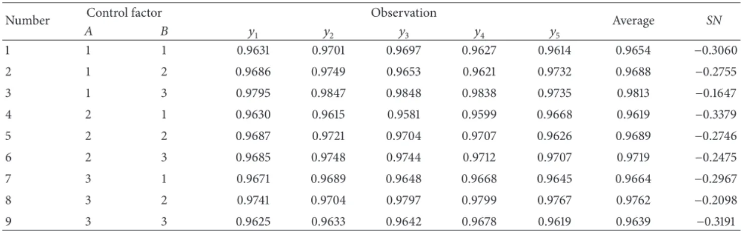
Table 4: Classification accuracy comparison.

Dermatology database Zoo database

𝐶 𝛾 𝐶 𝛾 1 3 10 12 0.1 5 10 12 1 52.57% 95.18% 94.08% 94.22% 1 71.18% 78.09% 62.36% 40.64% 10 52.57% 96.04% 97.94% 97.93% 10 71.18% 96.00% 91.00% 85.09% 50 52.57% 96.31% 96.86% 96.58% 50 71.18% 96.09% 96.00% 96.00% 100 52.57% 96.31% 96.32% 96.03% 100 71.18% 96.09% 96.09% 96.00%

Table 5: Factor level configuration of LS-SVM parameter design.

Dermatology database Zoo database

Control factor Level Control factor Level

1 2 3 1 2 3

𝐴(𝐶) 10 50 100 𝐴(𝐶) 5 10 50

𝐵(𝛾) 2.4 5 10 𝐵(𝛾) 0.08 4 11

4.3. Evaluation of Classification Accuracy. Cross-validation

measurement divides all the samples into a training set and a testing set. The training set is the learning data of the algorithm to establish the classification rules; the samples of the testing data are used as the testing data to measure the performance of the classification rules. All the samples are randomly divided into𝑘-folds by category, and the data are mutually repelled. Each fold of the data is used as the testing data and the remaining𝑘−1 folds are used as the training set. The step is repeated𝑘 times, and each testing set validates the classification rules learnt from the corresponding training set to obtain an accuracy rate. The average of the accuracy rates of all𝑘 testing sets can be used as the final evaluation results. The method is known as𝑘-fold cross-validation.

4.4. Results and Discussion. The ranking order of all features

for Dermatology and Zoo databases, using RFE-SVM, is summarized as follows: Dermatology ={V1, V16, V32, V28, V19, V3, V17, V2, V15, V21, V26, V13, V14, V5, V18, V4, V23, V11, V8, V12, V27, V24, V6, V25, V30, V29, V10, V31, V22, V20, V33, V7, V9} and Zoo = {V13, V9, V14, V10, V16, V4, V8, V1, V11, V2, V12, V5, V6, V3, V15, V7}. According to the suggestions of scholars, the classification error rate of OAO is relatively lower when the number of testing instances is below 1000. Multiclass SVM parameter settings can affect the Multi-class SVM’s Multi-classification accuracy. Arenas-Garc´ıa and P´erez-Cruz applied SVMs’ parameters setting in the multiclass Zoo dataset [31]. They have carried out simulation, using Gaussian kernels, for all possible combinations of𝐶 and Garmar from 𝐶 = [𝑙, 3, 10, 30, 100] and Garmar = sqrt(0.25d), sqrt(0.5d), sqrt(d), sqrt(2d), and sqrt(4d) with d being the dimension of the input data. In this study, we have executed wide ranges of the parameter settings for Dermatology and Zoo databases. Finally, the parameter settings are suggested as Dermatology (𝐶, 𝛾) = {𝐶 = 1, 10, 50, 100 and 𝛾 = 1, 3, 10, 12}, Zoo (𝐶, 𝛾) = {𝐶 = 1, 10, 50, 100 and 𝛾 = 0.1, 5, 10, 12}, and the testing accuracies are shown inTable 4.

As shown inTable 4, regarding parameter𝐶, when 𝐶 = 10 and 𝛾 = {5, 10, 12}, the accuracy of the experiment is higher than that of the experimental combination of𝐶 = 1

and 𝛾 = {5, 10, 12}; moreover, regarding parameter 𝛾, the experimental accuracy rate in the case of𝛾 = 5 and 𝐶 = {1, 10, 50, 100} is higher than that of the experimental com-bination of𝛾 = 0.1 and 𝐶 = {1, 10, 50, 100}. The near optimal value of𝐶 or 𝛾 may not be the same for different databases. Finding the appropriate parameter settings is important for the performance of classifiers. Practically, it is impossible to simulate every possible combination of parameter settings. And that is the reason why Taguchi methodology is applied to reduce the experimental combinations for SVM. The experimental step used in this study was first referred to the related study, ex,𝐶 = [1, 3, 10, 30, 100], [31]; then set a possible range for both databases (𝐶 = 1∼100, 𝛾 = 1∼12). After that, we slightly adjusted the ranges to understand if there will be better results in Taguchi quality engineering parameter optimization for each database. According to our experimental result, the final parameter settings𝐶 and 𝛾 range 10∼100 and 2.4∼10, respectively, for Dermatology database; the parameters settings𝐶 and 𝛾 range 5∼50 and 0.08∼11, respectively, for Zoo databases. Within the range of Dermatology and Zoo databases parameters𝐶 and 𝛾, we select three parameter levels and two control factors,𝐴 and 𝐵, to represent parameters 𝐶 and 𝛾, respectively. The Taguchi orthogonal array experiment selects𝐿₉(32) and the factor level configuration is as illustrated inTable 5.

After data preprocessing, Dermatology and Zoo databases include 358 and 101 testing instances, respectively. The various experiments of the orthogonal array are repeated five times (𝑛 = 5); the experimental combination and observations are summarized, as shown in Tables6 and 7. According to (13), we can calculate the𝑆𝑁 ratio for Taguchi experimental combination #1 as 𝑆𝑁LTB= −10 log₁₀[ 1 5 × ( 1 0.96312 + 1 0.97012 + 1 0.96972 + _0.96271 ₂ +_0.96141 ₂)] = −0.3060. (14)

(7)

Table 6: Summary of experiment data of Dermatology database.

Number Control factor Observation Average SN

𝐴 𝐵 𝑦1 𝑦2 𝑦3 𝑦4 𝑦5 1 1 1 0.9631 0.9701 0.9697 0.9627 0.9614 0.9654 −0.3060 2 1 2 0.9686 0.9749 0.9653 0.9621 0.9732 0.9688 −0.2755 3 1 3 0.9795 0.9847 0.9848 0.9838 0.9735 0.9813 −0.1647 4 2 1 0.9630 0.9615 0.9581 0.9599 0.9668 0.9619 −0.3379 5 2 2 0.9687 0.9721 0.9704 0.9707 0.9626 0.9689 −0.2746 6 2 3 0.9685 0.9748 0.9744 0.9712 0.9707 0.9719 −0.2475 7 3 1 0.9671 0.9689 0.9648 0.9668 0.9645 0.9664 −0.2967 8 3 2 0.9741 0.9704 0.9797 0.9799 0.9767 0.9762 −0.2098 9 3 3 0.9625 0.9633 0.9642 0.9678 0.9619 0.9639 −0.3191 (𝐴1= 10, 𝐴2= 50, 𝐴3= 100; 𝐵1= 2.4, 𝐵2= 5, 𝐵3= 10).

Table 7: Summary of experiment data of Zoo database.

Number Control factor Observation Average SN

𝐴 𝐵 𝑦₁ 𝑦₂ 𝑦₃ 𝑦₄ 𝑦₅ 1 1 1 0.9513 0.9673 0.9435 0.9567 0.9546 0.9547 −0.4037 2 1 2 0.9600 0.9616 0.9588 0.9611 0.9608 0.9605 −0.3504 3 1 3 0.7809 0.7833 0.7820 0.7679 0.7811 0.7790 −2.1694 4 2 1 0.7118 0.6766 0.7368 0.7256 0.7109 0.7123 −2.9571 5 2 2 0.9600 0.9612 0.9604 0.9519 0.9440 0.9555 −0.3960 6 2 3 0.8900 0.8947 0.9214 0.9050 0.9190 0.9060 −0.8598 7 3 1 0.7118 0.7398 0.7421 0.7495 0.7203 0.7327 −2.7064 8 3 2 0.9610 0.9735 0.9709 0.9752 0.9661 0.9693 −0.2709 9 3 3 0.9600 0.9723 0.9707 0.9509 0.9763 0.9660 −0.3013 (𝐴1= 5, 𝐴2= 10, 𝐴3= 50; 𝐵1= 0.08, 𝐵2= 4, 𝐵3= 11).

The calculation results of the𝑆𝑁 ratios of the remaining eight experimental combinations are summarized, as in Table 6. The Zoo experimental results and𝑆𝑁 ratio calculation are as shown inTable 7. According to the above results, we then calculate the average𝑆𝑁 ratios of the various factor levels. With the experiment ofTable 8 as an example, the average 𝑆𝑁 ratio 𝐴1of Factor𝐴 at Level 1 is

𝐴₁= 1₃[−0.3060 + (−0.2755) + (−0.1647)] = −0.2487. (15) Similarly, we can calculate the average effects of𝐴₂ and 𝐴₃fromTable 6. The difference analysis results of the various factor levels of Dermatology and Zoo databases are as shown inTable 8. The factor effect diagrams are as shown in Figures 2 and 3. As a greater 𝑆𝑁 ratio represents better quality, according to the factor level difference and factor effect diagrams, the Dermatology parameter level combination is 𝐴₁𝐵₃; in other words, parameters 𝐶 = 10, 𝛾 = 10, Zoo parameter level combination is 𝐴₁𝐵₂, and the parameter settings are𝐶 = 5, 𝛾 = 4.

When constructing the Multiclass SVM model using SVM-RFE, three different feature sets are selected according

−0.24 −0.25 −0.26 −0.27 −0.28 −0.29 −0.30 −0.31 −0.32 1 2 3 1 2 3 A B SN

Figure 2: Main effect plots for𝑆𝑁 ratio of Dermatology database.

to their significance. At the first stage, Taguchi quality engineering is applied to select the optimum values of parameters𝐶 and 𝛾. At the second stage, it constructs the Multiclass SVM Classifier and compares the classification performance according to the above parameters. In the Dermatology experiment,Table 9illustrates the two feature subsets containing 23 and 33 feature variables. The 33 feature

(8)

Table 8: Average of each factor at all levels.

Dermatology Zoo

Control factor Level Control factor Level

1 2 3 Difference 1 2 3 Difference

𝐴(𝐶) −0.2487 −0.2867 −0.2752 0.0380 𝐴(𝐶) −0.9745 −1.4043 −1.0929 0.4298

𝐵(𝛾) −0.3135 −0.2533 −0.2438 0.0697 𝐵(𝛾) −2.0224 −0.3391 −1.1102 1.6833

Table 9: Classification performance comparison of Dermatology database.

Methods Dimensions 𝐶 𝛾 Accuracy

SVM 33 100 5 95.10%± 0.0096

SVM-RFE 23 50 2.4 89.28%± 0.0139

SVM-RFE-Taguchi 23 10 10 95.38%± 0.0098

Table 10: Classification performance comparison of Zoo database.

Methods Dimensions 𝐶 𝛾 Accuracy

SVM 16 10 11 89%± 0.0314 SVM-RFE 6 50 0.08 92%± 0.0199 SVM-RFE-Taguchi 12 5 4 97%± 0.0396 3 2 1 1 2 3 −0.5 −1.0 −1.5 −2.0 A B SN

Figure 3: Main effect plots for𝑆𝑁 ratio of Zoo database.

sets are tested by SVM and SVM, as based on Taguchi. The parameter settings and testing accuracy rate results are as shown in Table 9. The experimental results, as shown in

Figure 4, show that the SVM (𝐶 = 10, 𝛾 = 10) testing

accuracy rate of the 17-feature sets datasets can be higher than 90%, which is better than the accuracy rate of 20-feature sets dataset SVM (𝐶 = 10, 𝛾 = 11), up to 90%. Moreover, regardless of how many sets of feature variables are selected, the accuracy of SVM (𝐶 = 50, 𝛾 = 2.4) cannot be higher than 90%.

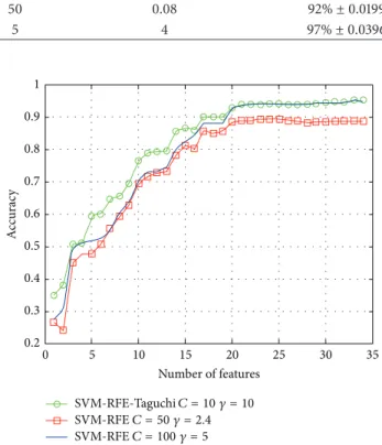
Regarding the Zoo experiment,Table 10summarizes the experimental test results of sets containing 6, 12, and 16 feature variables using SVM and SVM based on Taguchi. As shown in Table 10, the experimental results show that the classification accuracy rate of the set of 12-feature variables in the classification experiment using SVM-RFE-Taguchi (𝐶 = 10, 𝛾 = 10) is the highest, up to 97% ± 0.0396. As shown in Figure 5, the experimental results show that the classification

1 0.9 0.8 0.7 0.6 0.5 0.4 0.3 0.2 A cc u rac y 0 5 10 15 20 25 30 35 Number of features SVM-RFE-TaguchiC = 10 𝛾 = 10 SVM-RFEC = 50 𝛾 = 2.4 SVM-RFEC = 100 𝛾 = 5

Figure 4: Classification performance comparison of Dermatology database.

accuracy rate of the dataset containing 7 feature variables by SVM-RFE-Taguchi (𝐶 = 50, 𝛾 = 2.4) can be higher than 90%, which can obtain relatively better prediction effects.

5. Conclusions

As the study on the impact of feature selection on the multiclass classification accuracy rate becomes increasingly attractive and significant, this study applies SVM-RFE and SVM in the construction of a multiclass classification method in order to establish the classification model. As RFE is a

(9)

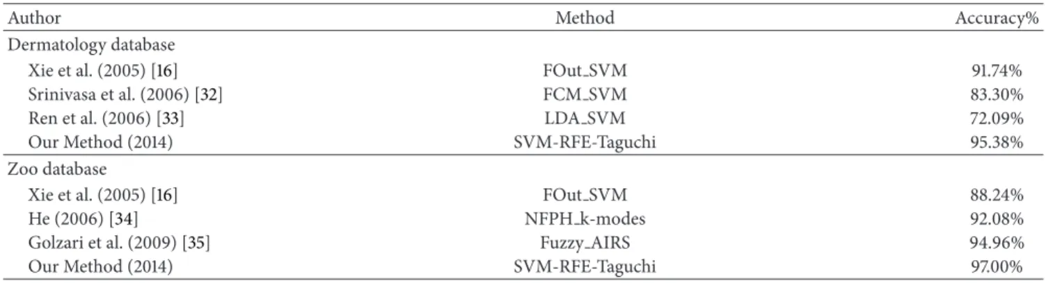
Table 11: Comparison of classification accuracy in related literature.

Author Method Accuracy%

Dermatology database

Xie et al. (2005) [16] FOut SVM 91.74%

Srinivasa et al. (2006) [32] FCM SVM 83.30%

Ren et al. (2006) [33] LDA SVM 72.09%

Our Method (2014) SVM-RFE-Taguchi 95.38%

Zoo database

Xie et al. (2005) [16] FOut SVM 88.24%

He (2006) [34] NFPH k-modes 92.08%

Golzari et al. (2009) [35] Fuzzy AIRS 94.96%

Our Method (2014) SVM-RFE-Taguchi 97.00%

1 0.95 0.9 0.85 0.8 0.75 0.7 0.65 A cc urac y 0 2 4 6 8 10 12 14 16 Number of features SVM-RFE-Taguchi_{C = 5 𝛾 = 4} SVM-RFEC = 10 𝛾 = 11 SVM-RFE_{C = 50 𝛾 = 0.08}

Figure 5: Classification performance comparison of Zoo database.

feature selection method of a wrapper model, it requires a previously defined classifier as the assessment rule of feature selection; therefore, SVM is used as the RFE assessment standard to help RFE in the selection of feature sets.

According to the experimental results of this study, with respect to parameter settings, the impact of parameter selection on the construction of SVM classification model is huge. Therefore, this study applies the Taguchi parameter design in determining the parameter range and selection of the optimum parameter combination for SVM classifier, as it is a key factor influencing the classification accuracy. This study also collected the experimental results of using different research methods in the case of Dermatology and Zoo databases [16,32,33], as shown inTable 11. By comparison, the proposed method can achieve higher classification accuracy.

Conflict of Interests

The authors declare that there is no conflict of interests regarding the publication of this paper.

References

[1] N. Cristianini and J. Shawe-Taylor, An Introduction to Support Vector Machines and Other Kernel-based Learning Methods, Cambridge University Press, Cambridge, UK, 2000.

[2] J. Luts, F. Ojeda, R. van de Plas Raf, B. de Moor, S. van Huffel, and J. A. K. Suykens, “A tutorial on support vector machine-based methods for classification problems in chemometrics,” Analytica Chimica Acta, vol. 665, no. 2, pp. 129–145, 2010. [3] M. F. Akay, “Support vector machines combined with feature

selection for breast cancer diagnosis,” Expert Systems with Applications, vol. 36, no. 2, pp. 3240–3247, 2009.

[4] C.-Y. Chang, S.-J. Chen, and M.-F. Tsai, “Application of support-vector-machine-based method for feature selection and clas-sification of thyroid nodules in ultrasound images,” Pattern Recognition, vol. 43, no. 10, pp. 3494–3506, 2010.

[5] H.-L. Chen, B. Yang, J. Liu, and D.-Y. Liu, “A support vector machine classifier with rough set-based feature selection for breast cancer diagnosis,” Expert Systems with Applications, vol. 38, no. 7, pp. 9014–9022, 2011.

[6] P. Danenas and G. Garsva, “Credit risk evaluation modeling using evolutionary linear SVM classifiers and sliding window approach,” Procedia Computer Science, vol. 9, pp. 1324–1333, 2012.

[7] C. L. Huang, H. C. Liao, and M. C. Chen, “Prediction model building and feature selection with support vector machines in breast cancer diagnosis,” Expert Systems with Applications, vol. 34, no. 1, pp. 578–587, 2008.

[8] H. F. Liau and D. Isa, “Feature selection for support vector machine-based face-iris multimodal biometric system,” Expert Systems with Applications, vol. 38, no. 9, pp. 11105–11111, 2011. [9] Y. Zhang, Z. Chi, and Y. Sun, “A novel multi-class support vector

machine based on fuzzy theories,” in Intelligent Computing: International Conference on Intelligent Computing, Part I (ICIC ’06), D. S. Huang, K. Li, and G. W. Irwin, Eds., vol. 4113 of Lecture Notes in Computer Science, pp. 42–50, Springer, Berlin, Germany.

[10] Y. Aksu, D. J. Miller, G. Kesidis, and Q. X. Yang, “Margin-maximizing feature elimination methods for linear and nonlin-ear kernel-based discriminant functions,” IEEE Transactions on Neural Networks, vol. 21, no. 5, pp. 701–717, 2010.

[11] P. Pudil, J. Novoviˇcov´a, and J. Kittler, “Floating search methods in feature selection,” Pattern Recognition Letters, vol. 15, no. 11, pp. 1119–1125, 1994.

(10)

[12] I. Guyon, J. Weston, S. Barnhill, and V. Vapnik, “Gene selec-tion for cancer classificaselec-tion using support vector machines,” Machine Learning, vol. 46, no. 1–3, pp. 389–422, 2002. [13] S. Harikrishna, M. A. H. Farquad, and Shabana, “Credit scoring

using support vector machine: a comparative analysis,” in Advanced Materials Research, Trans Tech Publications, Z¨urich, Switzerland, 2012.

[14] X. Lin, F. Yang, L. Zhou et al., “A support vector machine-recursive feature elimination feature selection method based on artificial contrast variables and mutual information,” Journal of Chromatography B: Analytical Technologies in the Biomedical and Life Sciences, vol. 10, pp. 149–155, 2012.

[15] R. Zhang and M. Jianwen, “Feature selection for hyperspectral data based on recursive support vector machines,” International Journal of Remote Sensing, vol. 30, no. 14, pp. 3669–3677, 2009. [16] Z. X. Xie, Q. H. Hu, and D. R. Yu, “Fuzzy output support

vector machines for classification,” in Advances in Natural Computation, L. Wang, K. Chen, and Y. S. Ong, Eds., vol. 3612, pp. 1190–1197, Springer, Berlin, Germany.

[17] Y. Liu, Z. You, and L. Cao, “A novel and quick SVM-based multi-class multi-classifier,” Pattern Recognition, vol. 39, no. 11, pp. 2258– 2264, 2006.

[18] J. Platt, N. C. Cristianini, and J. Shawe-Taylor, “Large margin DAGs for multiclass classification,” in Advances in Neural Information Processing Systems, S. A. Solla, T. K. Leen, and K. R. Muller, Eds., vol. 12, pp. 547–553, 2000.

[19] Y. Xu, S. Zomer, and R. G. Brereton, “Support vector machines: a recent method for classification in chemometrics,” Critical Reviews in Analytical Chemistry, vol. 36, no. 3-4, pp. 177–188, 2006.

[20] M. L. Huang, Y. H. Hung, and E. J. Lin, “Effects of SVM parameter optimization based on the parameter design of Taguchi method,” International Journal on Artificial Intelligence Tools, vol. 20, no. 3, pp. 563–575, 2011.

[21] H.-C. Lin, C.-T. Su, C.-C. Wang, B.-H. Chang, and R.-C. Juang, “Parameter optimization of continuous sputtering pro-cess based on Taguchi methods, neural networks, desirability function, and genetic algorithms,” Expert Systems with Applica-tions, vol. 39, no. 17, pp. 12918–12925, 2012.

[22] Y. Mao, D. Pi, Y. Liu, and Y. Sun, “Accelerated recursive feature elimination based on support vector machine for key variable identification,” Chinese Journal of Chemical Engineering, vol. 14, no. 1, pp. 65–72, 2006.

[23] A. Pal and J. Maiti, “Development of a hybrid methodology for dimensionality reduction in Mahalanobis-Taguchi system using Mahalanobis distance and binary particle swarm optimization,” Expert Systems with Applications, vol. 37, no. 2, pp. 1286–1293, 2010.

[24] C.-T. Su and Y.-H. Hsiao, “Multiclass MTS for simultane-ous feature selection and classification,” IEEE Transactions on Knowledge and Data Engineering, vol. 21, no. 2, pp. 192–205, 2009.

[25] X. Lin, F. Yang, L. Zhou et al., “A support vector machine-recursive feature elimination feature selection method based on artificial contrast variables and mutual information,” Journal of Chromatography B, vol. 910, pp. 149–155, 2012.

[26] E. H¨ullermeier and S. Vanderlooy, “Combining predictions in pairwise classification: an optimal adaptive voting strategy and its relation to weighted voting,” Pattern Recognition, vol. 43, no. 1, pp. 128–142, 2010.

[27] L. Bottou, C. Cortes, J. Denker et al., “Comparison of classifier methods—a case study in handwritten digit recognition,” in

Proceedings of the 12th Iapr International Conference on Pattern Recognition, vol. 2, pp. 77–82, IEEE Computer Society Press, Los Alamitos, Calif, USA, 1994.

[28] J. Furnkranz, “Round robin rule learning,” in Proceedings of the 18th International Conference on Machine Learning (ICML '01), pp. 146–153, 2001.

[29] M. R. Sohrabi, S. Jamshidi, and A. Esmaeilifar, “Cloud point extraction for determination of Diazinon: optimization of the effective parameters using Taguchi method,” Chemometrics and Intelligent Laboratory Systems, vol. 110, no. 1, pp. 49–54, 2012. [30] W. C. Hsu and T. Y. Yu, “Support vector machines parameter

selection based on combined taguchi method and staelin method for e-mail spam filtering,” International Journal of Engineering and Technology Innovation, vol. 2, no. 2, pp. 113–125, 2012.

[31] J. Arenas-Garc´ıa and F. P´erez-Cruz, “Multi-class support vector machines: A new approach,” in Proceeding of the IEEE Interna-tional Conference on Accoustics, Speech, and Signal Processing (ICASSP '03), vol. 2, pp. 781–784, April 2003.

[32] K. G. Srinivasa, K. R. Venugopal, and L. M. Patnaik, “Feature extraction using fuzzy c-means clustering for data mining sys-tems,” International Journal of Computer Science and Network Security, vol. 6, no. 3A, pp. 230–236, 2006.

[33] Y. Ren, H. Liu, C. Xue, X. Yao, M. Liu, and B. Fan, “Classification study of skin sensitizers based on support vector machine and linear discriminant analysis,” Analytica Chimica Acta, vol. 572, no. 2, pp. 272–282, 2006.

[34] Z. He, Farthest-point heuristic based initialization methods for K-modes clustering [thesis], Department of Computer Science and Engineering, Harbin Institute of Technology, Harbin, China, 2006.

[35] S. Golzari, S. Doraisamy, M. N. Sulaiman, and N. I. Udzir, “Effect of fuzzy resource allocation method on AIRS classifier accu-racy,” Journal of Theoretical and Applied Information Technology, vol. 5, no. 1, pp. 18–24, 2009.

(11)

Submit your manuscripts at

http://www.hindawi.com

Computer Games Technology International Journal of

Hindawi Publishing Corporation

http://www.hindawi.com Volume 2014

http://www.hindawi.com Volume 2014 Distributed Sensor Networks International Journal of Advances in

Fuzzy

Systems

International Journal of

Reconfigurable Computing

Applied

Computational

Intelligence and Soft

Computing

Advances in

Artificial

Intelligence

Hindawi Publishing Corporation http://www.hindawi.com Volume 2014 Advances in Software Engineering Hindawi Publishing Corporation

Electrical and Computer Engineering

Journal of

Computer Networks and Communications

Hindawi Publishing Corporation

http://www.hindawi.com Volume 2014

Multimedia

International Journal of

Biomedical Imaging

Artificial

Neural Systems

Advances in

Robotics

Journal of

http://www.hindawi.com Volume 2014 Hindawi Publishing Corporationhttp://www.hindawi.com Volume 2014

Computational Intelligence and Neuroscience

Modelling & Simulation in Engineering

The Scientific

World Journal

Human-Computer Interaction

Advances in

Computer EngineeringAdvances in