關於邊連通數和邊度數的問題 - 政大學術集成

全文

(1)國立政治大學應用數學系碩士學位論文. ‧. ‧ 國. 學. 政治大立 Some Topics on Edge Connectivity and Edge Degrees 關於邊連通數和邊度數的問題 n. er. io. sit. y. Nat. al. Ch. engchi. i Un. v. 碩士班學生：陳玫芳. 撰. 指導教授：張宜武博士中華民國一百年七月五日.

(2) Contents. Abstract. ii. 中文摘要. iii. 1 Introduction. 1. 2 Some Properties of Locally Connected Graphs and Locally Coconnected Graphs. 立. 2. 政治大. 3 The Number of Edge Cuts of k-regular Graphs. 7. ‧ 國. 學. 4 The Maximum Difference of the Minimum Edge Degree and the Minimum Vertex Degree of a Graph. 23. ‧ 28. sit. n. al. er. io. References. y. Nat. 5 Open Problems and Further Directions of Studies. Ch. engchi. i. i Un. v. 29.

(3) Abstract In this thesis, we classify some graphs into locally coconnected graphs or locally connected graphs, compute the number of its edge cuts of size 2k − 1 and 2k in a Harary graph, and show some properties of the number of vertices of degree 1 when the graph has the maximum difference of minimum edge degree and minimum vertex degree. keywords: Locally Connected Graphs; Edge Cuts; Restricted Edge Connectivity.. 立. 政治大. ‧. ‧ 國. 學. n. er. io. sit. y. Nat. al. Ch. engchi. ii. i Un. v.

(4) 中文摘要在這篇論文中，我們根據局部連通和局部補連通性質將圖分類，計算在 Harary 圖裡大小為 2k − 1 和 2k 邊切集的個數，和證明當圖形有最大的最小邊度數和最小點度數差，一些關於度數為 1 的點個數性質。關鍵詞：局部連通圖；邊切集；限制邊連通數。. 立. 政治大. ‧. ‧ 國. 學. n. er. io. sit. y. Nat. al. Ch. engchi. iii. i Un. v.

(5) 1. Introduction It is convenient to travel among cites by airplane, ship, or train. Every traffic. system is just a graph consisting of stations and routes. Nevertheless, if the system sometimes gets paralyzed at certain lines or certain locations because of earthquakes, tsunamis, or bad weathers, then we have to spend more time on traveling. Now, we put our attention on the connectivity among stations and the relationships of lines and stops. We follow [4] for notations in graph theory and define a graph G(V, E), where V = V (G) is the vertex set and E = E(G) is the edge set. It is very hard to. 治政大and introduce the definitions our focus on the neighborhood of a vertex in a graph of locally connected graphs立 and locally coconnected graphs. In chapter 3, we study study the connectivity of an arbitrary graph. Therefore, in chapter 2, we reduce. ‧ 國. 學. the number of the edge cut of a fixed size in k-regular graphs. Ou Jianping and Fuji Zhang provide some new ideas for counting it in [2]. They introduce optimal. ‧. graphs and super restricted edge connected graphs in order to show the number of the edge cuts of sizes less than 2k − 1. We extend the size of the edge cuts to 2k − 1. sit. y. Nat. and 2k, and get the number of the different edge cuts for specific Harary graphs. In chapter 4, we study the difference of the minimum edge degree and the minimum. io. er. vertex degree of a graph. When the graph has the maximum difference, we compute. al. n. iv n C the number of edges in these graphs. U up some open problems and h eFinally, n g c hwei bring further directions of research. the upper bound of the number of vertices with degree 1 and the lower bound of. 1.

(6) 2. Some Properties of Locally Connected Graphs and Locally Coconnected Graphs To determine the connectivity of any graph is actually difficult, so we reduce. the problem to study the connectivity of the neighborhood of a vertex. Definition 2.1. The graph G is called locally connected if the neighborhood NG (v) of every vertex v in G is connected. Definition 2.2. A vertex v of a graph G is called locally coconnected if the neigh¯ of G is connected. A graph G is called borhood NG (v) of v in the complement G. 政治大. locally coconnected if every vertex in G is locally coconnected.. 立. A locally connected city is very important to its neighbor zones. Let us see. ‧ 國. 學. some examples of locally conconnected graph.. Theorem 2.3. Every triangle-free graph is locally coconnected.. ‧. Proof. Let G be a triangle-free graph. For every vertex v of G, let N (v) denote the. Nat. n. al. er. io. sit. y. neighborhood of v in G. N (v) is an independent set. Then G is locally coconnected.. i Un. v. Corollary 2.4. Every bipartite graph is locally coconnected.. Ch. engchi. Proof. Since any bipartite graph G is triangle-free, G is locally coconnected by Theorem 2.3. A paw is defined to be a triangle with an additional vertex adjacent to one of the vertices of the triangle and the graph is drawn in Figure 1.. Figure 1: Paw.. 2.

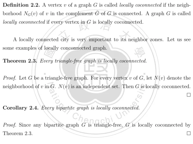
(7) Definition 2.5. A chord of a cycle C is an edge not in C whose endpoints lie in C. A chordless cycle in G is a cycle of length at least 4 in G that has no chord. A graph G is chordal if it is simple and has no chordless cycle. Theorem 2.6. Let G be a chordal graph with minimum degree δ(G) ≥ 2 and it contains no paw. Then G is a locally connected graph. Proof. Let x be any vertex of G. Because the degree d(x) of x is greater than or equal to 2, we have at least two vertices in N (x). If any two vertices are adjacent to each other, then G is locally connected. So, we may assume there exist two vertices u and v in N (x) such that u is not adjacent to v and consider the following two cases.. 政治大 Case 1: All u, v-paths contain x. Since the degree of each vertex in G is greater 立 than or equal to 2 and G is chordal, x is contained in a cycle C . Then it 3. ‧ 國. 學. forms a paw, which contradicts our assumption.. Case 2: There is a path u, v-path P that does not contain x. For any vertex w. ‧. in P , it is a neighbor of x because G has no Cn , n ≥ 4. If there is a vertex. y. Nat. y in N (x) and y does not belong to P , then the triangle x, u, w and edge xy. n. al. er. io. connected.. sit. form a paw in Figure 2, which contradicts to our assumption. Hence, N (x) is. Ch. engchi. i Un. v. Figure 2: The graph shows the relationship of the neighbors of the vertex x in G.. Definition 2.7. Three vertices v1 , v2 , v3 in a graph G form an asteroidal triple or AT of G if, for i, j ∈ {1, 2, 3} and i < j, there is a path from vi to vj which avoids using any vertex in the closed neighborhood N [vk ] = {vk } ∪ N (vk ).. 3.

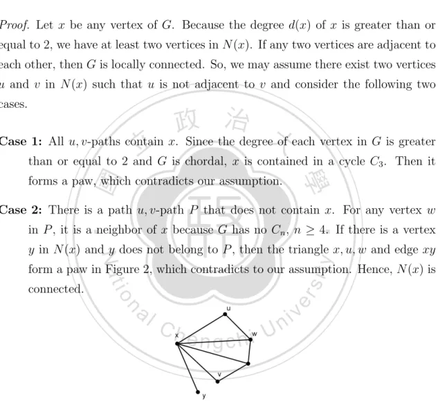
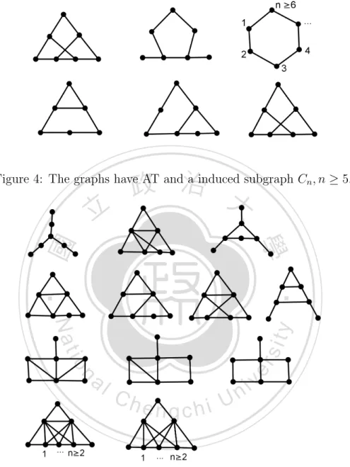
(8) An easy way to verify this for vertices v1 , v2 , v3 in a graph G is to examine whether v1 , v2 are connected in G − N [v3 ], v2 , v3 are connected in G − N [v1 ] ,and v1 , v3 are connected in G − N [v2 ]. Ekkehard G. K¨ohler shows an important theorem about the AT-free graph in [3]. Lemma 2.8. A graph G is AT-free if and only if it does not contain any of the graphs in Figure 3 as induced subgraph.. 立. 政治大. ‧. ‧ 國. 學. n. er. io. sit. y. Nat. al. Ch. engchi. i Un. v. Figure 3: The structure of forbidden subgraphs of asteroidal triple-free graphs. Theorem 2.9. Let G be a graph without Cn , n ≥ 5 and K1,3 as an induced subgraph. ¯ is a locally coconnected graph. G has AT and δ(G) ≥ 2. Then G Proof. Let G be a graph with AT. Then G has induced subgraphs in Figure 3 and we have to check the assumptions in them. The graphs in Figure 4 contain Cn , n ≥ 5 as an induded subgraph, the graph in Figure 5 have an induced subgraph K1,3 , and there exist some vertices with degree 1 in Figure 6. The only graphs which satisfy. 4.

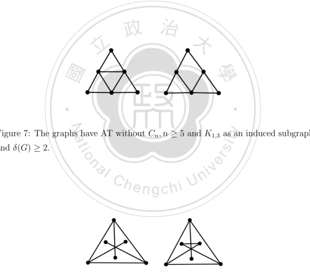
(9) the conditions are in Figure 7 and the complement of them in Figure 8. It is obvious that every vertex in Figure 8 is locally coconnected.. 政治大. Figure 4: The graphs have AT and a induced subgraph Cn , n ≥ 5.. 立. ‧. ‧ 國. 學. n. er. io. sit. y. Nat. al. Ch. engchi. i Un. v. Figure 5: The graphs have AT and a induced subgraph K1,3 .. 5.

(10) Figure 6: The graphs have AT and some vertices with degree 1.. 立. 政治大. ‧. ‧ 國. 學 y. Nat. n. al. er. io. and δ(G) ≥ 2.. sit. Figure 7: The graphs have AT without Cn , n ≥ 5 and K1,3 as an induced subgraph. Ch. engchi. i Un. v. Figure 8: The graphs are the complement of graphs which have AT without Cn , n ≥ 5 and K1,3 as an induced subgraph and δ(G) ≥ 2.. 6.

(11) 3. The Number of Edge Cuts of k-regular Graphs First, we give some condition to an edge cut of a graph G and observe the. relationship between the conditional edge connectivity and the minimal edge degree. Abdol-Hossein Esfahanian and S. Louis Hakimi studied the conditional edge connectivity in [1]. In this chapter, we call a disconnected graph, a triangle, or a star trivial and all other graphs non-trivial. Definition 3.1. Let G be a non-trivial simple graph and S ⊆ E(G). The set S is called a restricted edge cut of G if G − S is disconnected and each component has at least two vertices. The restricted edge connectivity λ0 (G) of G, is defined as the. 政治大 Definition 3.2. Let G be a simple graph. For an edge e = xy in G, we denote 立 ξ(e) = d(x) + d(y) − 2 and call the ξ(G) = min{ξ(e)|e ∈ E(G)} as minimum edge. minimum size of all restricted edge cuts of G.. ‧ 國. 學. degree of G.. Nat. λ0 (G) ≤ ξ(G).. sit. y. inequality. ‧. Obviously, for any non-trivial graph G, λ0 (G) exists and satisfies the following. al. er. io. Definition 3.3. Let G be a non-trivial simple graph. We say G is optimal if. n. the equality λ0 (G) = ξ(G) holds; otherwise G is non-optimal. We call G is super. Ch. i Un. v. restricted edge connected if G − S has a component consisting of an isolated edge. engchi. for every restricted edge cut S of the minimum size in G. A graph G is called k-regular if every vertex of G has degree k. In the following statements, the graph G is simple if not specially stated. Jun-Ming Xu and Ke-Li Xu had some research for optimal and non-optimal graphs in [5]. It is clearly to see that super restricted edge connected graphs are optimal, but the converse is not true. Ou Jianping and Fuji Zhang showed that a sufficient condition for k-regular graphs to be optimal and super restricted edge connected. Lemma 3.4. [2] Let G be a k-regular connected graph of order n. (i) If k >. n , then G is optimal. 2 7.

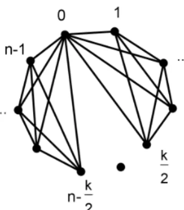
(12) (ii) If k >. n + 1, then G is super restricted edge connected. 2. When we study the system reliability, we often focus on the model whose nodes never fail but lines have a breakdown independently of each other with equal probability. Suppose every station has the same number of branches and the system n is very dense, then we describe it as a k-regular graph with k > + 1 . After some 2 edges are broken such that the graph decomposes into more than one component, we call the edge set as an edge cut. When the size of an edge cut is not more than 2k − 2, we only consider the component which is a single vertex or an isolated edge by Lemma 3.4. In a graph G, we use the notation Ch to be the number of its edge cuts of size h in G.. 政治大. Theorem 3.5. [2] Let G be a connected k-regular graph of order n. If k >. , if h = k . 學. , if k < h < 2k − 2. . ‧. . y.  + nk , if h = 2k − 2. 2. io. n. er. Nat. al. , if h < k. sit. 立.   0      n      nk   −k n 2 Ch =  h−k      nk   −k    n 2   k−2. ‧ 國. then. n + 1, 2. i Un. v. In [4], given k < n, the construction of Harary graphs Hk,n is to place n. Ch. engchi. vertices uniformly around a circle and label the vertices by the integers modulo n, k each vertex is adjacent to the nearest vertices in clockwise and counterclockwise 2 k−1 vertices in directions if k is even, and each vertex is adjacent to the nearest 2 each direction and to the diametrically opposite vertex if k is odd and n is even. In these two cases, Hk,n is a k-regular graph. When k and n are both odd, the n−1 n−1 structure of Hk,n is Hk−1,n adding the edges i ↔ i + for 0 ≤ i ≤ . It 2 2 indicates that every vertex has degree k except one vertex with degree k − 1. n It is convenient to call an edge xy in Hk,n as diagonal edge if |x − y| = . In 2 ! n addition, given n, r ∈ Z, we define the notation to be zero if r < 0. In the r following statement, we compute the number of triangles in Hk,n .. 8.

(13) Lemma 3.6. Let T (k, n) be the number of triangles in Hk,n and t n2 be the number of triangles containing a diagonal edge.  k (i) If k is even, then T (k, n) = n  2  + t0 , where 2 . t0 =. n [ 3. n−1. !. n−3. .  k  n− 2 −1  −3   +3 k n− −3 2. n−k−1. !. n−k−3.  3  n − 2k − 1  − ]. 3 n− k−3 2 .  k−1 (ii) If k is odd and n is even, then T (k, n) = n  2  + t0 + t n2 , where 2 .    n k−1 n − −1  −k 2 2 ]. + n 2 n k−1 −k−1 − −2 2 2 2. n. er. io. al. n−k−2. ‧. Nat.   n  −1 2  − 2 t n2 = n[ n  −2 2. n−k. y. n−3. 立.  n− 2 −1  −3  +3 k−1 −3 n− 2. .  3  n − 2k  − ] 3 n− k−2 2. !. sit. n−1. 政治 大 k−1. 學. and. n [ 3. ‧ 國. t0 =. !. . i Un. v. Proof. (i) Let k be even. We name the distance d between two vertices x, y in Hk,n as the following. Ch. engchi. d = minimum{|x − y|, n − |x − y|}. For any three vertices in Hk,n , every vertex is incident to two edges, say two hands, of this triangle. Hence, we consider the following two cases. If two hands of a vertex x are incident to neighbors of x in the clockwise direction, then there is an edge adjacent two neighbors of x since the distance of any k two neighbors of x in the same direction is less than . It is similar for the 2  k  2  × 2 triangles in counterclockwise direction, so each vertex provides 2 Figure 9.. 9.

(14) Figure 9: The graph shows that each vertex in Hk,n has triangles in the same. 政治大 In addition, every triangle is counted two times, so there are 立  . direction of hands.. ‧ 國.  k = n 2  2 . ‧. 2. 學. k  2 ×2 n 2. y. Nat. triangles. If two hands of a vertex are in the different directions, then we have. sit. the following model. n. al. er. io. x1 + x2 + x3 = n k 1 ≤ x1 , x2 , x3 ≤ , 2 where x1 , x2 , and x3 are the distances between every pair of vertices of trian-. Ch. engchi. i Un. v. gles in Hk,n . We solve the model by using the generating function k. g(x) = (x + x2 + ... + x 2 )3 k. = x3 (1 + x + ... + x 2 −1 )3 k. 1 − x2 3 =x ( ) 1−x k 1 3 = x3 ( ) (1 − x 2 )3 . 1−x 3. Moreover, we have the polynomial expansions ! ! 3 4 1 3 ) =1+ x+ x2 + ... + ( 1−x 1 2. 10. r+2 r. ! xr + ....

(15) and k. k. 3. (1 − x 2 )3 = 1 − 3x 2 + 3xk − x 2 k . The coefficient cn−3 of xn−3 in g(x) is   ! k n−1  n− 2 −1  − 3 +3 k n−3 n− −3 2. .  3 n−k−1  n − 2k − 1  − . 3 n−k−3 n− k−3 2 n Since every triangle is counted three times, we get t0 = × cn−3 triangles. 3 !. (ii) Let k be odd and n be even. By similar argument, we consider three cases for each vertex, two hands are in the same direction, two hands are in different directions, or the triangle has a diagonal edge.  If two hands  of a vertex are k−1 in the same direction, then each vertex provides  2  × 2 triangles. In 2 addition, every triangle is counted two times, so there are   k−1   n 2  × 2 k−1 2 = n 2  2 2. 立. 政治大. ‧. ‧ 國. 學. y. Nat. triangles. If two hands of a vertex are in the different directions, then we have. sit. the following model. n. al. er. io. x1 + x2 + x3 = n k−1 1 ≤ x1 , x2 , x3 ≤ , 2 where x1 , x2 , and x3 are the distances between every pair of vertices of trian-. Ch. engchi. i Un. v. gles in Hk,n . We solve the model by using the generating function g(x) = (x + x2 + ... + x. k−1 2. = x3 (1 + x + ... + x. )3. k−1 −1 2. )3. k−1. 1−x 2 3 =x ( ) 1−x k−1 1 3 = x3 ( ) (1 − x 2 )3 . 1−x 3. The coefficient cn−3 of xn−3 in g(x) is   ! k−1 n−1  n− 2 −1  − 3 +3 k−1 n−3 n− −3 2 11. n−k n−k−2. !. .  3  n − 2k  − . 3 n− k−2 2.

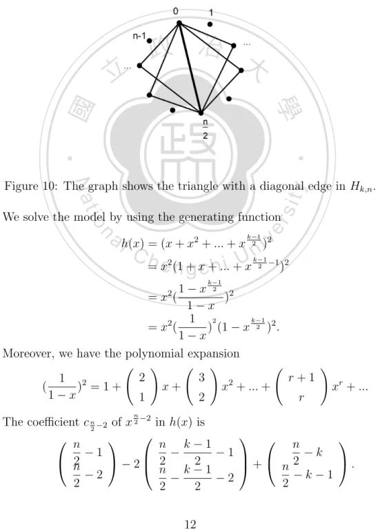
(16) n × cn−3 triangles. 3 If the triangle contains a diagonal edge xy in the Figure 10, then we find a. Since every triangle is counted three times, we get t0 =. common neighbor z of x and y to form a triangle and yields the following model n 2 k−1 1 ≤ x1 , x2 ≤ , 2 where x1 and x2 are the distances between every pair of vertices of triangles x1 + x2 =. in Hk,n .. 政治大. 立. ‧. ‧ 國. 學. Nat. sit. y. Figure 10: The graph shows the triangle with a diagonal edge in Hk,n .. er. io. We solve the model by using the generating function. n. a lh(x) = (x + x2 + ... + x )i2v n Ch 2 =e xn (1 g + xc+h...i +Ux −1 )2 k−1 2. k−1 2. k−1. 1−x 2 2 =x ( ) 1−x k−1 1 2 = x2 ( ) (1 − x 2 )2 . 1−x Moreover, we have the polynomial expansion ! ! ! 2 3 r + 1 1 2 ( ) =1+ x+ x2 + ... + xr + ... 1−x 1 2 r 2. n. The coefficient c n2 −2 of x 2 −2 in h(x) is     n   n k−1 n −1 − − 1 − k   2 2 2 2  n  − 2 .  n + n k − 1 −2 − k − 1 − −2 2 2 2 2 12.

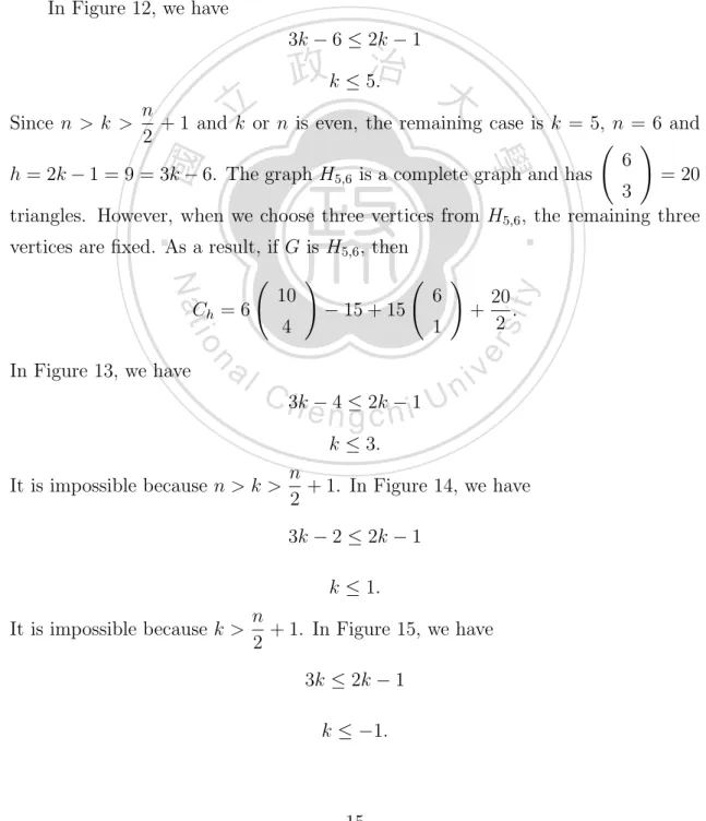
(17) Since x and y have a corresponding common neighbor in the other direction n n and there are diagonal edges, we get t n2 = 2× ×c n2 −2 = n×c n2 −2 triangles. 2 2. Now, we extend Theorem 3.5 to h = 2k − 1 and h = 2k, and the k-regular graph is restricted to a Harary graph. When cutting more edges in a graph, a smaller component can be a single vertex, an isolated edge, a triangle, or K4 . We need Lemma 3.6 to compute the number of triangles in these cases and the number of triangles that are counted twice. Theorem 3.7. Let G be a Harary graph Hk,n with k >. 政治大. n + 1 and h = 2k − 1. If k 2. or n is even, then      nk nk     2 − k  − nk + nk  2 − 2k + 1  , if G is not H5,6    n 2 2 k−1 1 Ch = ! !   10 6 20   − 15 + 15 + , if G is H5,6 .   6 2 4 1. 立. ‧. ‧ 國. 學. y. Nat. sit. n. al. er. io. Proof. Let S be an edge cut of Hk,n and G − S has a component with p vertices, n where p ≤ b c. Since k or n is even, Hk,n is a k-regular graph and it implies that 2 nk there are edges. If p is 1, then S is a disjoint union of two edge sets. One consists 2 of k edges incident to a single vertex chosen from Hk,n and the other contains k − 1 nk edges chosen arbitrarily from the remaining −k edges of Hk,n . However, when we 2 cut all incident edges of two vertices which are adjacent  to each other,  see Figure 11, nk − k  nk this edge cut is counted two times. Hence, there are n  2 − ways. 2 k−1. Ch. engchi. i Un. v. If p is 2, then S is composed of 2k − 2 edges incident to a specific edge chosen nk from edges in Hk,n and one edge in the remaining edges. As a result, there are 2  nk − 2k + 1  nk  2 ways. If p is 3, then Hk,n has at least six vertices and we 2 1 have four following cases about this three vertices of Hk,n in Figure 12, Figure 13, Figure 14, Figure 15.. 13.

(18) Figure 11: Two adjacent vertices in Hk,n have 2k − 1 incident edges.. 立. 政治大. ‧ 國. 學. Figure 12: Three vertices x, y, z of Hk,n are adjacent to each other and there are additional 3k − 6 edges which are incident to x, y, z.. ‧. n. er. io. sit. y. Nat. al. Ch. engchi. i Un. v. Figure 13: The graph of three vertices x, y, z of Hk,n forms a path and there are additional 3k − 4 edges which are incident to x, y, z.. Figure 14: Two of three vertices x, y, z of Hk,n are adjacent and there are additional 3k − 2 edges which are incident to x, y, z.. 14.

(19) Figure 15: Three vertices x, y, z of Hk,n form an independent set and there are additional 3k edges which are incident to x, y, z. In Figure 12, we have 3k − 6 ≤ 2k − 1. 政k ≤ 治 5. 大. 立. n + 1 and k or n is even, the remaining case is k = 5, n = 6 and 2 ! 6 h = 2k − 1 = 9 = 3k − 6. The graph H5,6 is a complete graph and has = 20 3 triangles. However, when we choose three vertices from H5,6 , the remaining three Since n > k >. n. al. 1. y. ! +. 20 . 2. sit. 6. er. io. In Figure 13, we have. ‧. ‧ 國. 學. Nat. vertices are fixed. As a result, if G is H5,6 , then ! 10 Ch = 6 − 15 + 15 4. C h3k − 4 ≤ 2k − 1 U n i engchi. v. k ≤ 3. It is impossible because n > k >. n + 1. In Figure 14, we have 2 3k − 2 ≤ 2k − 1 k ≤ 1.. It is impossible because k >. n + 1. In Figure 15, we have 2 3k ≤ 2k − 1 k ≤ −1.. 15.

(20) It is impossible. If p > 3, then we have p. pk − 2. ! ≤ 2k − 1. 2. p(p − 1) ≤ 2k − 1 2 (p − 2)k ≤ p(p − 1) − 1 1 k ≤p+1+ p−2 n +1<k ≤p+1 2 n < 2p. pk − 2 ×. 政治大. n − p ≤ p − 1 ≤ (n − p) − 1,. 立. which is a contradiction. Therefore, G − S has a smaller component which is either. Theorem 3.8. Let G be a Harary graph Hk,n with k >. n + 1 and h = 2k. If k or 2. ‧. ‧ 國. 學. a single vertex or an isolated edge when G is not H5,6 .. n. al. Ch. engchi U. er. io. (i) If G is not H5,6 , H6,7 , H6,8 , or H6,9 , then     nk nk − k  nk  − 2k + 1  2 Ch = n  2 − −( 2 k 1. sit. y. Nat. n is even, then the following statements are true.. v! n in 2.  nk − 2k + 1  nk nk − )+  2 . 2 2 2 . (ii) If G is H5,6 , then 10. Ch = 6. !. 5. − 15. 6. ! −(. 1. 6. ! − 15) + 15. 2. 6. !. 2. + 60.. (iii) If G is H6,7 , then Ch = 7. 15 6. ! − 21. 10 1. ! −(. 16. 7 2. ! − 21) + 21. 10 2. ! + 35..

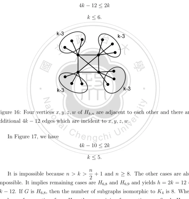
(21) (iv) If G is H6,8 , then Ch = 8. 18. ! − 24. 6. 13. ! −(. 1. 8. ! − 24) + 24. 2. 13. ! + 32 + 4.. 2. (v) If G is H6,9 , then Ch = 9. 21. ! − 27. 6. 16. ! −(. 1. 9. !. 2. − 27) + 27. 16 2. ! + 30 + 9.. Proof. Let S be an edge cut of Hk,n and G − S has a component with p vertices, n where p ≤ b c. Since k or n is even, Hk,n is a k-regular graph and it implies that 2 nk there are edges. 2. 政治大 If p is 1, then S is a disjoint union of two edge sets. One consists of k edges 立 incident to a vertex chosen from H and the other contains k edges chosen ark,n. ‧ 國. 學. nk bitrarily from the remaining − k edges of Hk,n . However, there are two cases 2 in which some triangles are counted two times. One is cutting all incident edges. ‧. of two vertices which are adjacent to each other plus an extra edge, and the other. n. al. er. io. sit. y. Nat. is cutting all incident which are  not adjacent to each other.  edges oftwo vertices  ! nk nk n − k − 2k + 1 nk nk  2 − −( Hence, there are n  2 ) ways. − 2 2 2 k 1. i Un. v. If p is 2, then S is composed of 2k − 2 edges incident to a specific edge chosen nk from edges in Hk,n and two edges in the remaining edges. As a result, there are  2 nk − 2k + 1  nk  2 ways. 2 2. Ch. engchi. By an argument similar to the one of Theorem 3.7, if p is 3, then Hk,n has at least six vertices and we only need to consider the case S contains 3k − 6 edges incident to a triangle in Hk,n . It yields the following inequalities 3k − 6 ≤ 2k k ≤ 6. When k = 6, h = 2k = 12 = 3k − 6 and we have three cases H6,7 , H6,8 and H6,9 n since n > k > + 1. By Lemma 3.6, there are T (6, 7) = 35, T (6, 8) = 32, and 2 17.

(22) T (6, 9) = 30 triangles, respectively. When k = 5, h = 2k = 10 = (3k − 6) + 1 and n we get the case H5,6 since n > k > + 1 and k or n is even. As we pick a triangle in 2 ! 6 T (5, 6) H5,6 , the remaining three vertices are fixed. Hence, there are × = 60 2 1 ways. If p is 4, then Hk,n has at least eight vertices and we consider the case in Figure 16. We have 4k − 12 ≤ 2k k ≤ 6.. 立. 政治大. ‧. ‧ 國. 學 sit. y. Nat. al. er. io. Figure 16: Four vertices x, y, z, w of Hk,n are adjacent to each other and there are. n. additional 4k − 12 edges which are incident to x, y, z, w. In Figure 17, we have. Ch. engchi. i Un. v. 4k − 10 ≤ 2k k ≤ 5. n + 1 and n ≥ 8. The other cases are also 2 impossible. It implies remaining cases are H6,8 and H6,9 and yields h = 2k = 12 = It is impossible because n > k >. 4k − 12. If G is H6,8 , then the number of subgraphs isomorphic to K4 is 8. When we choose four vertices from H6,8 , then remaining four vertices are fixed. Hence, 8 there are = 4 ways. If G is H6,9 , then the number of subgraphs isomorphic to K4 2 is 9.. 18.

(23) Figure 17: Four vertices x, y, z, w of Hk,n are adjacent to each other except one pair vertices and there are additional 4k − 10 edges which are incident to x, y, z, w.. 政治大 !. If p > 4, then we have. p. pk − 2. ≤ 2k. 2. p(p − 1) ≤ 2k 2 (p − 2)k ≤ p(p − 1) 2 k ≤p+1+ p−2 n +1<k ≤p+1 2 n < 2p. 學. ‧ 國. 立. pk − 2 ×. n. engchi. y. sit er. io. Ch. ‧. Nat. al. i Un. v. n − p ≤ p − 1 ≤ (n − p) − 1,. which is a contradiction. Therefore, G − S has a smaller component which is either a single vertex or an isolated edge when G is not H5,6 , H6,7 , H6,8 , or H6,9 . If G is H5,6 , then Ch = 6. 10. !. 5. − 15. 6. ! −(. 1. 6. ! − 15) + 15. 2. 6. !. 2. + 60.. If G is H6,7 , then Ch = 7. 15 6. ! − 21. 10 1. ! −(. 19. 7 2. ! − 21) + 21. 10 2. ! + 35..

(24) If G is H6,8 , then 18. Ch = 8. ! − 24. 6. 13. ! −(. 1. 8. !. 13. − 24) + 24. 2. ! + 32 + 4.. 2. If G is H6,9 , then 21. Ch = 9. ! − 27. 6. 16. ! −(. 1. 9 2. !. 16. − 27) + 27. !. 2. + 30 + 9.. After cutting a specific number of edge from a k-regular graph, we observe the remaining components.. 立. 政治大. Theorem 3.9. Let G be a k-regular connected graph of order n. We obtain two. ‧ 國. 學. components A and B by removing ξ(G) edges from G and 1 < |A| ≤ |B|. (i) If n is odd and k =. ‧. n+1 , then |A| = 2 or |A| + 1 = |B| > 3. In particular, A 2. is a clique.. Nat. n + 1, then |A| = 2 or |A| = |B| > 2. In particular, if 2 |A| > 2 ,then A and B are cliques.. n. al. er. io. sit. y. (ii) If n is even and k =. i Un. v. Proof. (i) If |A| = 2, then A is K2 and we are done. So, we consider the case n+1 n |A| > 2. Since k = > , G is optimal by Lemma 3.4. That is 2 2 λ0 (G) = ξ(G) = 2k − 2 = n − 1. After we cut n − 1 edges in G, it forms two n−1 components A and B and |A| ≤ . In addition, G is a k-regular graph, 2 n+1 so every vertex in A has at least k − (|A| − 1) = − |A| + 1 neighbors 2 which belong to B in G. n−1 . Since |A| > 2, multiply both sides by |A| − 2 and we Assume |A| < 2 obtain n−1 (|A| − 2)|A| < (|A| − 2) 2 n−1 (|A| − 2)|A| < |A| × − (n − 1) 2 n−1 |A|( − (|A| − 2)) > n − 1 2. Ch. engchi. 20.

(25) n+1 − |A| + 1) > n − 1. 2 It means that there are more than n − 1 edges between A and B in G, which |A|(. is a contradiction to the fact that A and B are disconnected after removing n−1 n − 1 edges in G. So, we get |A| = and |B| = |A| + 1. 2 n+1 If A is not a clique, then every vertex in A has more than − |A| + 1 2 neighbors in B. We obtain more than |A|(. n−1 n+1 n−1 n+1 − |A| + 1) = ( − + 1) = n − 1 2 2 2 2. edges between A and B in G which contradicts to our assumption. Hence, A is a clique.. 治政 (ii) If |A| = 2, then we are done. So, we consider大 the case |A| > 2. Since k = n n 立 by Lemma 3.4. That is λ (G) = ξ(G) = 2k − 2 = n. + 1 > , G is optimal 2 2 0. ‧. ‧ 國. 學. After we cut n edges in G, it forms two components A and B and |A| ≤ n . In addition, G is a k-regular graph, so every vertex in A has at least 2 n n k − (|A| − 1) = ( + 1) − |A| + 1 = − |A| + 2 neighbors which belong to B 2 2 in G. n Assume |A| < . Since |A| > 2, multiply both sides by |A| − 2 and we obtain 2. n. er. io. n 2. sit. y. Nat. al. (|A| − 2)|A| < (|A| − 2). v C(|A|h − 2)|A| < |A| ×Unn−i n engchi 2. n − (|A| − 2)) > n 2 n |A|( − |A| + 2) > n. 2 It means that there are more than n edges between A and B in G, which is |A|(. a contradiction to the fact that A and B are disconnected after removing n n edges in G. So, we get |A| = and |B| = |A|. 2 n If A is not a clique, then every vertex in A has more than −|A|+2 neighbors 2 in B. We obtain more than |A|(. n n n n − |A| + 2) = ( − + 2) = n 2 2 2 2. 21.

(26) edges between A and B which contradicts to our assumption. Hence, A is n2 n a clique and there are − edges in A. We need to n edges in order to 8 4 separate A and B. We can compute the number of edges in B by |E(G)| − |E(A)| − n =. nk n2 n n2 n −( − )−n= − . 2 8 4 8 4. So, B is also a clique.. 立. 政治大. ‧. ‧ 國. 學. n. er. io. sit. y. Nat. al. Ch. engchi. 22. i Un. v.

(27) 4. The Maximum Difference of the Minimum Edge Degree and the Minimum Vertex Degree of a Graph In this chapter, we study the difference of the minimum edge degree ξ(G) and. the minimum vertex degree δ(G) of a graph G, say m00 = ξ(G)−δ(G). For example, every path of length at least 2 has m00 = 1 − 1 = 0 and the complete graph of order n , n > 1, has m00 = 2(n − 1) − 2 − (n − 1) = n − 3. Theorem 4.1. Let G be a simple graph without isolated vertices. Then the maximum of m00 is n − 3.. 政治大 and w be a vertex of G with minimum vertex degree δ(G) = d(w). Since G has no 立 isolated vertices, we can find a vertex z in G adjacent to w. Then. Proof. Let uv be an edge of G with minimum edge degree ξ(G) = d(u) + d(v) − 2. ‧ 國. 學. m00 = (d(u)+d(v)−2)−δ(G) ≤ (d(w)+d(z)−2)−δ(G) ≤ δ(G)+(n−1)−2−δ(G) = n−3.. of m00 is n − 3.. ‧. In addition, the complete graph of order n, n > 1, has m00 = n−3. So, the maximum. sit. y. Nat. Lemma 4.2. Let G be a simple graph of order n without isolated vertices and has. n. al. er. io. m00 = n − 3. If the vertex v in G has minimum vertex degree, then for any neighbor u of v has degree n − 1.. Ch. engchi. i Un. v. Proof. Since G is a simple graph, d(u) ≤ n − 1. The minimum edge degree ξ(G) is less than or equal to d(v) + d(u) − 2 and m00 = ξ(G) − δ(G) = ξ(G) − d(v) = n − 3. We have d(u) ≥ n − 1. Hence, the degree of u is n − 1. In a simple graph of order n without isolated vertices and m00 = n − 3, the vertex with minimum degree is adjacent to the vertex with maximum degree and it is a connected graph. Theorem 4.3. Let G be a simple graph of order n without isolated vertices and has n−3 m00 = n − 3. If G is not a star, then p ≤ d e, where p is the number of vertices 2 with degree 1.. 23.

(28) Proof. Let v be a vertex in G with minimum degree and u be a neighbor of v. By Lemma 4.2, the degree of u is n − 1, that is, u is adjacent to every vertex in G except itself. Let S = {x ∈ V (G)|d(x) = 1} and G0 = G − S − {u}. Because G is not a star, G0 has at least an edge wz in Figure 18.. 政治大. 立. ‧ 國. 學. Figure 18: The graph shows the relationship between the maximum degree u and. ‧. the subgraph G0 in G.. io. sit. y. n−3 e. 2. er. Nat. Suppose p = |S| > d. n 1 n−3 n 1 Case 1: If n is odd, then p ≥ + 1 = − and |V (G0 )| ≤ n − ( − ) − 1 = 2 2 2 2 2 n 1 − . Then we have the inequality, 2 2. n. al. Ch. ξ(G) ≤ d(w) + d(z) − 2 ≤ (. engchi. i Un. v. n 1 n 1 − − 1 + 1) + ( − − 1 + 1) − 2 = n − 3. 2 2 2 2. It contradicts to ξ(G) − δ(G) = n − 3. n−3 3 n n n + = and |V (G0 )| ≤ n − − 1 = − 1. 2 2 2 2 2 Then we have the inequality,. Case 2: If n is even, then p ≥. ξ(G) ≤ d(w) + d(z) − 2 ≤ (. n n − 1 − 1 + 1) + ( − 1 − 1 + 1) − 2 = n − 4. 2 2. It contradicts to ξ(G) − δ(G) = n − 3. Hence, p ≤ d. n−3 e. 2 24.

(29) If G is a star with order n, then m00 = (n − 2) − 1 = n − 3. However, the n−3 e. In the number of vertices with degree 1 is n − 1 which is greater than d 2 following discussion, we use the same notation, S = {x ∈ V (G)|d(x) = 1} and G0 = G − S − {u} . Theorem 4.4. Let G be a simple graph of order n without isolated vertices and has m00 = n − 3. (i) If n is even and p = |S| = d (ii) If n is odd and p = |S| = d. n−3 e, then G0 is K n2 . 2. n−3 e, then G0 is K n + 1 or K n + 1 − e. 2 2 2 2 2. 治 n n n 政 − 1 and |V (G )| = n − ( − 1) − 1 = . If the 大 2 2 2 0. Proof. (i) Suppose n is even, p =. 立. order of G0 is 2, then G0 is K2 . Suppose G0 has at least 3 vertices and there. ‧ 國. 學. exist two vertices w, z in G0 such that w is not adjacent to z, for any edge yz in G0 , we have. n n − 1 + 1) + ( − 2 + 1) − 2 = n − 3. 2 2. ‧. ξ(G) ≤ d(y) + d(z) − 2 ≤ (. sit. y. Nat. It contradicts to ξ(G) − δ(G) = n − 3.. n 3 n 3 n 1 − and |V (G0 )| = n − ( − ) − 1 = + . If 2 2 2 2 2 2 the order of G0 is 2 or 3, then G0 is K2 , K3 or K3 − e, respectively. Suppose ¯0 , we have the G0 has at least 4 vertices and there are two edges e1 , e2 in G. n. al. er. io. (ii) Suppose n is odd, p =. following two cases.. Ch. engchi. i Un. v. Case 1: Assume e1 , e2 have the same endpoint w in G0 . Because d(w) > 1, there exists a vertex z which is adjacent to w in G as the following Figure 19. We have n 1 n 1 ξ(G) ≤ d(w) + d(z) − 2 ≤ ( + − 3 + 1) + ( + − 1 + 1) − 2 = n − 3. 2 2 2 2 It contradicts to ξ(G) − δ(G) = n − 3. Case 2: Assume e1 , e2 have different endpoints in G0 , say e1 = xy and e2 = ¯0 , then it is back to Case 1. Hence, wz. If xz, xw, yz, or yw are edges in G. 25.

(30) we consider x, y, z, w are pairwise adjacent to each other except x, y and w, z as in Figure 20, then n 1 n 1 ξ(G) ≤ d(x) + d(z) − 2 ≤ ( + − 2 + 1) + ( + − 2 + 1) − 2 = n − 3. 2 2 2 2 It contradicts to ξ(G) − δ(G) = n − 3. Therefore, G0 is K n + 1 or K n + 1 − e. 2. 立. 2. 2. 2. 政治大. Figure 19: The edges e1 , e2 in G0 have the same endpoint.. ‧. ‧ 國. 學. n. er. io. sit. y. Nat. al. Ch. i Un. v. Figure 20: The edge e1 , e2 in G0 have different endpoints.. engchi. A star with order n has n − 1 edges. Now, we discuss the lower bound of number of edges when the graph of order n has m00 = n − 3. Theorem 4.5. Let G be a simple graph of order n without isolated vertices and has m00 = n − 3. If G is not a star, then G has at least 2n − 4 edges. Proof. Case 1: If S is not an empty set, then the minimum vertex degree δ(G) is 1 and ξ(G) = n − 2. Now, we compute the number of edges in G0 . Since G is not a star, there is a vertex x in G0 . Without loss of generality, let x be the. 26.

(31) vertex with maximum vertex degree dG0 (x) = d in G0 , 1 ≤ d ≤ n − 3. If d is 1, then ξ(G) is 2. Because ξ(G) − δ(G) is n − 3, it implies that n is 4 and G is a paw. A paw has 4 edges and we are done. It remains to prove the case d ≥ 2. For a neighbor y of x in G0 , we have n − 2 = ξ(G) ≤ d(x) + d(y) − 2 d(x) + d(y) ≥ n. It implies dG0 (x) + dG0 (y) ≥ n − 2 and dG0 (y) ≥ n − d − 2. Thus, the number of edges in G0 is at least dG0 (x) +. P. dG0 (y). d + d(n − d − 2) . 2 2 It implies that there exist at least n − 3 edges in G0 . Therefore, we get y∈NG0 (x). =. 政治大. |E(G)| = |E(G0 )| + d(u) ≥ (n − 3) + (n − 1) = 2n − 4. The bound is. 立. best possible since the equality holds for the graph G in which |S| = 1 and. ‧. ‧ 國. 學. maximum vertex degree in G0 is n − 3 as in the Figure 21.. n. er. io. sit. y. Nat. al. Ch. engchi. i Un. v. Figure 21: The graph shows that there are n − 3 edges in G0 . Case 2: If S is an empty set, then the degree of every vertex in G is greater than 1. Suppose the vertex x in G has minimum vertex degree d, 2 ≤ d ≤ n − 1. For a neighbor y of x in G, the degree of y is n − 1 by Lemma 4.2. Thus, the number of edges in G is at least P P d(x) + y∈N (x) d(y) + z∈G−N (x)−{x} d(z) 2 Hence, we get |E(G)| ≥ 2n − 4.. 27. =. d + d(n − 1) + (n − d − 1)d . 2.

(32) 5. Open Problems and Further Directions of Studies In this article, we prove some graphs are locally connected or locally cocon-. nected, compute the number of edge cuts with size 2k − 1 and 2k in a Harary graph Hk,n , and show that the upper bound of the number of vertices with degree 1 and the lower bound of the number of edges in the graph with maximum difference of minimum edge degree and minimum vertex degree. There are still some open problems for future studies. 1. In Chapter 2, we have known some classes of locally connected graphs or locally coconnected graphs. Furthermore,. 治政大with these properties. a. We would like to characterize more graphs 立 b. We would like to study the relationship of a locally connected graph and ‧ 國. 學. a connected graph.. 2. When we enlarge the size of an edge cut, it is more difficult to predict the. ‧. remaining graph.. y. Nat. sit. a. We would like to find out the method of counting the number of Ks ’s. io. al. n. larger size.. er. with s ≥ 4 in a Harary graph and count the number of edge cuts with. Ch. i Un. v. b. We would like to count the number of edge cuts with a larger size in other k-regular graphs.. engchi. 28.

(33) References [1] A.-H. Esfahanian and S. L. Hakimi, On computing a conditional edgeconnectivity of a graph, Information Processing Letters, 27 (1988), pp. 195–199. [2] O. Jianping and F. Zhang, Super restricted edge connectivity of regular graphs, Graphs and Combinatorics, 21 (2005), pp. 459–467. ¨ hler, Graphs Without Asteroidal Triples, PhD thesis, Technischen [3] E. G. Ko Universit¨at Berlin, 1999. [4] D. B. West, Introduction to Graph Theory, Prentice Hall, 2001.. 政治大 Mathematics, 243 (2002), 立 pp. 291–298.. [5] J.-M. Xu and K.-L. Xu, On restricted edge-connectivity of graph, Discrete. ‧. ‧ 國. 學. n. er. io. sit. y. Nat. al. Ch. engchi. 29. i Un. v.

(34)