從序列回憶到再認：Serial-Order in a Box的延伸 - 政大學術集成

全文

(1)國立政治大學心. 理. 學. 系. 碩士論文. 治. 政從序列回憶到再認：Serial-Order 大 in a Box的延伸. 立. sit. io. 研究生：林軒宇 a l 指導教授：顏乃欣博士 v i 楊立行博士 n C. n. er. Nat. y. ‧. ‧ 國. 學. From Recall to Recognition: An Extension of Serial Order in a Box Model. hengchi U. 中華民國一百年六月.

(2) 從序列回憶到再認：Serial-Order in a Box的延伸 From Recall to Recognition: An Extension of Serial Order in a Box Model 研究生：林軒宇. Student: Hsuan-Yu Lin. 指導教授：顏乃欣博士. Advisor: Dr. Nai-Shing Yen. 楊立行博士. 治政大學國立政治大心. 理. 學. 系. 學. ‧ 國. 立. Dr. Lee-Xieng Yang. 碩士論文. ‧. A Thesis. y. Nat. n. al. College of Science. er. io. sit. Submitted to Department of Psychology. iv. Nactional Chengchi University n C. hengchi U. in Partial Fulfillment of the Requirements for the Degree of Master of Philosophy in Department of Psychology June 2011 Taipei City, Taiwan. 中華民國一百年六月.

(3) 立. 政治大. ‧. ‧ 國. 學. n. er. io. sit. y. Nat. al. Ch. engchi. i n U. v.

(4)

(5) 從序列回憶到再認：Serial-Order in a Box的延伸學生：林軒宇. 指導教授：顏乃欣博士楊立行博士國立政治大學心理學系摘. 要. 常久以來，序列回憶與再認被視為兩個不同的心理歷程，被分別的研究與探討。. 治政大因此本研究假設這兩個作業使用了相同的登入歷程與記憶表徵，只有在進行提立取時的歷程有所不同。為了驗證本研究假設，原先用來模擬序列回憶作業的類. 然而這兩個作業不僅有相似的實驗程序，受試者在作業的表現上也相當類似，. ‧ 國. 學. 神經網路模型Serial–Order in a Box (SOB) (Farrell & Lewandowsky, 2002)與其後繼C-SOB(Farrell, 2006; Lewandowsky & Farrell, 2008)被加以延伸，使其能夠進行. ‧. 再認。延伸的模型保留了SOB中的網路結構與登入歷程，僅使用了不同的提取歷. y. Nat. 程，便得以模擬再認作。此研究發現序列回憶與再認並不如先前認為的不相同歷. n. er. io. al. sit. 程，而是有相同的登入歷程與記憶表徵。. Ch. engchi. iv. i n U. v.

(6) From Recall to Recognition: An Extension of Serial Order in a Box Model Student: Hsuan-Yu Lin. Advisor: Dr. Nai-Shing Yen Dr. Lee-Xieng Yang. Submitted to Department of Psychology College of Science Nactional Chengchi University ABSTRACT. 政治大 Serial recall and recognition 立 are usually studied separately. However, it is reasonable. ‧ 國. 學. to assume that those two processes have the same encoding process and representation in memory trace, due to the fact that the two tasks share a similar experimental regime and similar behavioral findings. In this study, the difference between. ‧. those tasks is thought to be the retrieval process. In order to verify this hypothe-. sit. y. Nat. sis, a successful serial order recall model, Serial–Order in a Box (SOB) (Farrell &. io. er. Lewandowsky, 2002), and its successor, C-SOB (Farrell, 2006; Lewandowsky & Farrell, 2008), are extended to account for recognition. By keeping the encoding process. n. al. Ch. i n U. v. and structure in SOB unchanged, the performance of recognition task can be mod-. engchi. eled by modifying only retrieval process. This finding supports the assumption that serial recall and recognition share the same encoding process and representation.. v.

(7) Table of Content 書名頁 . . . . . . . . . . . . . . . . . . . . . . . . . . . . . . . . . . . . . . . .. i. 授權書 . . . . . . . . . . . . . . . . . . . . . . . . . . . . . . . . . . . . . . . .. ii. 論文口試委員審定書 . . . . . . . . . . . . . . . . . . . . . . . . . . . . . . . .. iii. 摘要 . . . . . . . . . . . . . . . . . . . . . . . . . . . . . . . . . . . . . . . . .. iv. Abstract . . . . . . . . . . . . . . . . . . . . . . . . . . . . . . . . . . . . . . .. v. Table of Content . . . . . . . . . . . . . . . . . . . . . . . . . . . . . . . . . .. vi. 立. 政治大. List of Tables . . . . . . . . . . . . . . . . . . . . . . . . . . . . . . . . . . . . viii. ‧ 國. 學. List of Figures . . . . . . . . . . . . . . . . . . . . . . . . . . . . . . . . . . .. ix. ‧. 符號說明 . . . . . . . . . . . . . . . . . . . . . . . . . . . . . . . . . . . . . . xii. Nat. sit. n. al. er. Recall and recognition . . . . . . . . . . . . . . . . . . . . . . . . . .. io. 1.1. y. 1. Introduction . . . . . . . . . . . . . . . . . . . . . . . . . . . . . . . . . . .. Ch. i n U. v. 1 1. 1.1.1. Serial recall task . . . . . . . . . . . . . . . . . . . . . . . . .. 1. 1.1.2. Sternberg’s task . . . . . . . . . . . . . . . . . . . . . . . . . .. 6. 1.2. Mental process in serial recall and recognition tasks . . . . . . . . . .. 9. 1.3. Computational modeling . . . . . . . . . . . . . . . . . . . . . . . . . 12. engchi. 2. Serial–Order in the Box and C-SOB . . . . . . . . . . . . . . . . . . . . . . 16 2.1. 2.2. Serial-Order in a Box model . . . . . . . . . . . . . . . . . . . . . . . 16 2.1.1. Encoding process . . . . . . . . . . . . . . . . . . . . . . . . . 17. 2.1.2. Retrieval process . . . . . . . . . . . . . . . . . . . . . . . . . 18. C-SOB model . . . . . . . . . . . . . . . . . . . . . . . . . . . . . . . 19. vi.

(8) 2.2.1. Encoding process . . . . . . . . . . . . . . . . . . . . . . . . . 22. 2.2.2. Recall process in serial recall . . . . . . . . . . . . . . . . . . . 23. 3. SOB model for recognition . . . . . . . . . . . . . . . . . . . . . . . . . . . 25 3.1. The extension of SOB and C-SOB . . . . . . . . . . . . . . . . . . . . 26 3.1.1. Measuring energy of probe . . . . . . . . . . . . . . . . . . . . 27. 3.1.2. Placing decision criterion of energy . . . . . . . . . . . . . . . 32. 政治大 Discussion . . . . . . . . . . . . . . . . . . . . . . . . . . . . . . . . . 立. 3.2. Simulation method and results . . . . . . . . . . . . . . . . . . . . . . 33. 3.3. 34. ‧ 國. Corbin and Macquar’s finding . . . . . . . . . . . . . . . . . . . . . . 38. io. y. Simulation of distant/recent negatives . . . . . . . . . . . . . 43. al. n. v i n Extralist–featureC effect . . . . . . i. .U. . . . . . . . . . . . . . . . . . hen gch. 4.3.1 4.4. sit. Distant/recent negatives . . . . . . . . . . . . . . . . . . . . . . . . . 42 4.2.1. 4.3. Simulations of Corbin and Macquar’s finding . . . . . . . . . . 41. Nat. 4.2. ‧. 4.1.1. Conclusion . . . . . . . . . . . . . . . . . . . . . . . . . . . . . . . . . 50 . . . . . . . . . . . . . . . . . . . . . . . . . . . . . . . 52. C-SOB . . . . . . . . . . . . . . . . . . . . . . . . . . . . . . . . . . . 53 5.1.1. 5.2. 45. Simulation of extralist–feature effect . . . . . . . . . . . . . . 46. 5. General discussion 5.1. er. 4.1. 學. 4. Follow up simulations . . . . . . . . . . . . . . . . . . . . . . . . . . . . . . 38. Simulations . . . . . . . . . . . . . . . . . . . . . . . . . . . . 53. Future works . . . . . . . . . . . . . . . . . . . . . . . . . . . . . . . 55. Reference . . . . . . . . . . . . . . . . . . . . . . . . . . . . . . . . . . . . . . 56. vii.

(9) List of Tables 3.1. The best fitting parameters for both model. . . . . . . . . . . . . . . 34. 4.1. The stimulus and negative probe design in Mewhort and Johns(2000)’s Experiment 1. Table adapted from Mewhort and Johns(2000)’s Table 1. . . . . . . . . . . . . . . . . . . . . . . . . . . . . . . . . . . . . . . 46 The stimulus and negative probe design in Mewhort and Johns(2000)’s. 政治大 . . . . . . . . . . . . . . . . . . . . . . . . . . . . . . . . . . 立. Experiment 1. Table adapted and reformed from Mewhort and Johns(2000)’s Table 3.. 學 ‧. ‧ 國 io. sit. y. Nat. n. al. er. 4.2. Ch. engchi. viii. i n U. v. 46.

(10) List of Figures 1.1. The procedure of serial recall task with list length 3. . . . . . . . . .. 1.2. The serial position effect in serial recall task. This figure is adapted. 2. from the left pannel of Figure 2 in Lewandowsky and Farrell (2008) .. 3. 1.3. The procedure of recognition task with list length 3. . . . . . . . . . .. 6. 1.4. The results from Sternberg(1969)’s experiment 1, adopted from Stern-. 政治大. berg(1969)’s Figure 4. . . . . . . . . . . . . . . . . . . . . . . . . . . 1.5. 立. The serial position curve in recognition task. This figure is adapted. ‧ 國. 學. from McElree and Dosher (1989)’s Figure 9. . . . . . . . . . . . . . . 1.6. 7. 8. The experiment procedure in Oberauer (2003). Each row represents. ‧. one display on screen. Presenting sequence is from top to bottom.. y. Nat. Items are presented in random order during learning phrase. While. io. sit. testing, a question mark cue shows in a frame. Participant has to. n. al. er. recall previous items presented in the frame. This figure is adapted. i n U. from the Figure 1 in Oberauer (2003). 1.7. Ch. engchi. v. . . . . . . . . . . . . . . . . . 10. Serial position curves in serial presentation condition in Oberauer (2003). This figure is adapted from Oberauer (2003)’s figure 2. . . . . 11. 2.1. The energy and encoding strength curve among different serial position in SOB. . . . . . . . . . . . . . . . . . . . . . . . . . . . . . . . . 18. 2.2. The structure of SOB. . . . . . . . . . . . . . . . . . . . . . . . . . . 20. 2.3. The energy and encoding strength curve among different serial position in C-SOB. . . . . . . . . . . . . . . . . . . . . . . . . . . . . . . 23. 3.1. The energy of positive probe and negative probe among different set sizes in SOB. . . . . . . . . . . . . . . . . . . . . . . . . . . . . . . . 27 ix.

(11) 3.2. The energy position curve among different serial position. . . . . . . . 28. 3.3. The energy of positive probe and negative probe among different set sizes in C-SOB. . . . . . . . . . . . . . . . . . . . . . . . . . . . . . . 30. 3.4. The energy position curve among different set size and serial position. 30. 3.5. Two different method to place decision criterion. Left figure is the constant criterion. Right figure is the linear criterion. Dash–dot line indicates the decision criterion. Solid line and dot line are the mean energy of positive probe and negative probe, respectively. Errorbar. 政治大. is one standard deviation of mean energy. . . . . . . . . . . . . . . . . 33 3.6. 立. The response tendency among serial position of four models. The up-. ‧ 國. 學. per left and figures show the response tendency of SOB with constant and linear criterion, respectively. The button left and right figures. The mean response tendency of four models. The upper left and. y. Nat. 3.7. ‧. show the response tendency for constant and linear criterion in C-SOB. 35. io. sit. figures show the response tendency of SOB with constant and linear. n. al. er. criterion, respectively. The button left and right figures show the. i n U. v. response tendency for constant and linear criterion in C-SOB. . . . . 36. 4.1. Ch. engchi. The RT of recognition in additional serial recall/recognition only condition. Figure is adapted from Corbin and Macquar (2008)’s figure 2.. 39. 4.2. The encoding strength (ηe ) from different ϕe . . . . . . . . . . . . . . . 40. 4.3. The probability of correct (P C) in serial recall task from different tc .. 4.4. The response tendency of changing ϕe or tc among different setsize.. 40. Upper figure shows the response tendency of different ϕe . Lower one shows the response tendency of different tc . . . . . . . . . . . . . . . . 41 4.5. The similarity between context for within trials context and between context. . . . . . . . . . . . . . . . . . . . . . . . . . . . . . . . . . . 44. x.

(12) 4.6. The simulation result of distant/recent negatives. . . . . . . . . . . . 45. 4.7. The representation of content layer for simulating extralist–feature effect. . . . . . . . . . . . . . . . . . . . . . . . . . . . . . . . . . . . 47. 4.8. The simulation for Mewhort and Johns (2000)’s Experiment 1. . . . . 47. 4.9. The redesigned representation of content layer for simulating extralist– feature effect. . . . . . . . . . . . . . . . . . . . . . . . . . . . . . . . 48. 4.10 The energy and response tendency of the simulation with redesigned. 政治大 4.11 The response tendency of the simulation with redesigned representa立 tion for Mewhort and Johns (2000)’s study. . . . . . . . . . . . . . . .. representation for Mewhort and Johns (2000)’s Experiment 1. . . . . 49. ‧. ‧ 國. 學. n. er. io. sit. y. Nat. al. Ch. engchi. xi. i n U. v. 50.

(13) 符號說明 vi. vector for item i.. sc. similiarity between each items.. pi. vector for item i’s position marker.. tc. similiarity between items’ position markers.. W. auto-associative network of content layer.. C. hetro-associative network between content and context layer.. ϕe. energy scale parameter for encoding.. ‧ 國. al. n. tp. Ch. er. standard deviation of noise.. sit. y. updating parameter in deblurring process.. io. σ0. preservation parameter in deblurring process.. Nat. α. energy of item i.. ‧. γ. 學. Ei. 立. 政治大. i n U. v. similiarity between probe’s position marker and last item’s position marker.. engchi. q. energy scaling parameter in EZ-diffusion model. T er. non-decision time in EZ-diffusion model. a. decision boundary in EZ-diffusion model. xii.

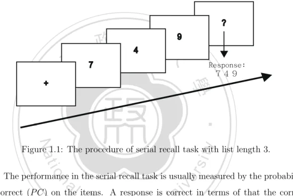
(14) 1.. Introduction. Memory is one of the most well-discussed field in cognitive psychology. Researchers in the past one hundred years have devoted to understanding the nature of it, including how we represent what we experience and how we encode and retrieve them. Among the various memory phenomena, recall and recognition are the two most studied. Also, there have been proposed a great deal of models respectively for each of these two phenomena. In the past researches, these two kinds of memory were often addressed separately. However, these two kinds of memory might not be com-. 政治大 processing of human cognition and the evidence implying shared mental process 立. pletely separated, according to the common understanding about the information. and representation between them. The principal goal of this study is to examine. ‧ 國. 學. this possibility via computer simulation and modeling. The main hypothesis of this study is that the processes of recall and recognition actually have the same encod-. ‧. ing process and form the same representation, with the retrieval process as the only. sit. y. Nat. difference. In order to verify this hypothesis, a contemporary successful model for serial recall, the SOB (Serial–Order in a Box) model, will be extended to accounting. io. n. al. er. for recognition results. Specifically, in accordance with the hypothesis, the encoding. i n U. v. process and the representation generating mechanism in SOB model for serial recall. Ch. engchi. will be remained in the series of modeling. Only will the retrieval process of the SOB model be modified to suit the recognition task. The hypothesis will be supported if the behavioral results of recognition can be accommodated by such a modified model.. 1.1 1.1.1. Recall and recognition Serial recall task. Since Ebbinghaus (1885) studied how well the learned items could be memorized along time, human recall process has been widely investigated. There are various. 1.

(15) kinds of recall task developed for different purposes, such as free recall, cued recall, forward recall, backward recall and so forth. Among these recall tasks, the serial recall task is one of the most typical case in examining recall performance in STM (Short-Term Memory). Normally, in doing the serial recall task, participants will be given a list of items (e.g., digits, characters, or words) to learn and asked to recall them in their presenting orders after learning. An example of the experimental procedure of serial recall task can be seen in Figure 1.1.. ?. 立. 9 政治 4 大 Response: ７４９. 7. ‧. ‧ 國. 學. +. y. Nat. er. io. sit. Figure 1.1: The procedure of serial recall task with list length 3. The performance in the serial recall task is usually measured by the probability. n. al. Ch. i n U. v. of correct (P C) on the items. A response is correct in terms of that the correct. engchi. item is recalled in the correct position in the memory list. The P C of item typically varies along the item position in the memory list. The P C is higher at the beginning of serial position (the primacy effect), lowest at mid of memory list, and rising at the end of the list (the recency effect), as a U-shape curve in Figure 1.2. Plenty theories of serial recall are conducted to explain the wealthful phenomena found by previous studies. Many theories go into computation model level and proposed different assumptions in detail about representations of memory, encoding/retrieval processes, and sources of errors, and their assumptions are supported/rejected by carefully designed experiments. The following section describes the major arguments between those models. The representations of memory trace mainly concerned in models are what 2.

(16) Proportion Correct. 1.0. 0.8. 0.6. 0.4. 0.2. 0.0. 治政 Serial 大 Position 1. 立. 2. 3. 4. 5. 6. 7. ‧ 國. 學. Figure 1.2: The serial position effect in serial recall task. This figure is adapted from the left pannel of Figure 2 in Lewandowsky and Farrell (2008). ‧. participants learded for certain task. In serial recall task, participants have to. sit. y. Nat. remember both the items in the trial and the serial order of those items. Different. io. er. models purpose different nature of how serial position is memorized. Generally, three types of representation are used for memorizing serial position: chaining, position. al. n. marker, and ordinal.. Ch. engchi. i n U. v. Chaining models assume that the serial position is coded by the association between neighbor items (Lewandowsky & Murdock, 1989; Elman, 1990). In the chainging model purposed by Lewandowsky and Murdock (1989), current presenting item and the association between the current and the previous item are encoded to the same memory storage. The first and the last item are associated with the start and end signal for each trial, respectively. While recalling, the start signal is served as the retrieval cue to retrieve the first reponse. The retrieved item is then used for retrieving following item as retrieval cue. This cycle continues till the ending signal is retrieved. Models with position markers propose that serial position is memorized through the association between items and markers with positional information. The posi-. 3.

(17) tion marker could be the temporal-based context or event-based context. In OSCAR (Brown, Hulme, & Preece, 2000), context markers which items associate with are generated by a set of oscillators which gradually change with time. Similiar temporal-based context is adapted in the phonological loop model proposed by Burgess and Hitch (1999) and SIMPLE (Brown, Neath, & Chater, 2002, 2007). Event-based context, unlike temporal-based context changes with time passing, evolves through event happening. C-SOB (Farrell, 2006; Lewandowsky & Farrell, 2008) and SEM (Henson, 1998) adopte event-based markers. In C-SOB model, the context which associates with item gradually changes with item presenting. There. 政治大. are two contexts mark the start and the end of trial in SEM, and those contexts have similiar role as the context in C-SOB. Regardless the base of context, the retrieval. 立. process is quite similar as that the context is treated as retrieval cue for response.. ‧ 國. 學. However, the difference in inter-item interval does not influence the prediction of event-based context models but temporal-based context. This difference is exam-. ‧. ined by the studies around teimpral isolation effect (Morin, Brown, & Lewandowsky, 2010). Temporal-based models predict that the temporal isolated items should per-. y. Nat. sit. form better than crowded items. In contract, event-based models predict no tempo-. al. er. io. ral isolation effect. Researches do find temporal isolation effect in serial recall and. v. n. suggest that memory trace consists of temporal information (Morin et al., 2010).. Ch. engchi. i n U. Ordinal models suggest that positional informaion is not memorized through item-item associaions or item-context associations but primacy gradient and response supression (Page & Norris, 1998; Farrell & Lewandowsky, 2002). Primacy gradient is that the encoding strength gradually decreases along with serial position. While retrieval, the item with hightest activation (eg., first item) is most likely to be responsed. Responsed item is then supressed from memory trace, thus the second item becomes the hightest activated and is most likely to be recalled next. There is no specific representation of serial order in ordinal models, instead the encoding and retrieval mechanism along are enough for reporting items serially. Primacy gradient and response supression are essential functions in ordinal models and also adopted in many context models. OSCAR , C-SOB, and SEM both have primacy gradient while encoding. However, it is important to note that the 4.

(18) course of primacy gradient is only explaimed by SOB (Farrell & Lewandowsky, 2002) and C-SOB (Farrell, 2006; Lewandowsky & Farrell, 2008). In both models, primacy gradient is the consquence of energy-gated encoding. Energy-gated encoding served as that the novelty of incomming information (energy) will modulate the encoding strength of incomming item. The novel items are encoded with greater strength, and the familiar items are encoded lighter. The more items storaged in memory trace, the more overlapping between incomming item and previous storaged memory trace and results in lesser novelty for later items. Interference from the other items in the memory trace is one of the major. 政治大 trieving process will be interference by the non-target chains and items since that 立 source of error in the models previous mentioned. In the chaining model, the re-. every information are stored in the same place. In position marker models, similiar. ‧ 國. 學. mechanism is applied as that the context-item association crosstalk to each other and cause interference while the context cue is used for retrieval. In ordinal model,. ‧. like Primacy model, the activation of item is noisy, and the item with highest acti-. sit. y. Nat. vation is responsed. The target item, theoretically should be the highest activated item, has to compete with remaining items because of the activation is noisy (Page. io. n. al. er. & Norris, 1998). The interference of non-target items happens in the deblurring. i n U. v. process in SOB model with similiar fasion (Farrell & Lewandowsky, 2002). Besides. Ch. engchi. interference, decay is also a common mechanism that couses error in serial recall. The activation of item decays over time, and the influence from noise increases along with more decay (Page & Norris, 1998; Burgess & Hitch, 1999). The debate between decay and interference is one of the heavly discussed topic in memory, and the evidence from researches did not converge. Some researches support that forgetting in retrieval is cuased by interference not decay (Oberauer & Lewandowsky, 2008; Lewandowsky & Oberauer, 2009; Brown & Lewandowsky, 2010), and some researches against this (Portrat, Barrouillet, & Camos, 2008).. 5.

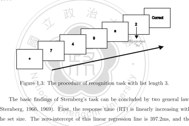
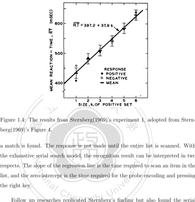
(19) 1.1.2. Sternberg’s task. In recognition, Sternberg’s memory scanning paradigm is the most classical paradigm. In the original task, participants are successively presented a list of single digits to learn, followed by another digit (i.e., the probe). The participants are asked to judge if the probe was presented in the memory list as quickly as possible (Sternberg, 1966, 1969). The paradigm is shown in Figure 1.3. If the probe is actually presented in the memory list, then it is called the positive probe, otherwise it is called the negative probe.. 立. 政治大. 2. * 4. 學. 9. ‧ 國. Correct. Response “No”. 7. ‧. +. sit. y. Nat. io. er. Figure 1.3: The procedure of recognition task with list length 3.. al. n. v i n (Sternberg, 1966, 1969). C First, response time (RT) is linearly increasing with h ethe ngchi U the set size. The zero-intercept of this linear regression line is 397.2ms, and the. The basic findings of Sternberg’s task can be concluded by two general laws. slope is 37.9 ms for each additional item in memory list. Second, the slope of RT for “yes” response is equal to “no” response. The result is shown in Figure 1.4. The similar results are replicated with characters, artificial symbols, words, and colors (Sternberg, 1975). Sternberg explains this finding with his exhaustive serial search model (Sternberg, 1966, 1969). In his model, the items in the memory list are marked with special markers serially during initial learning. When determining if the probe has been presented or not, a high-speed exhaustive scanning process compares the item in the list with the probe serially. If a match is found, then response is “yes”, and response is “no” otherwise. However, the scanning process does not stop even when. 6.

(20) 立. 政治大. ‧ 國. 學. Figure 1.4: The results from Sternberg(1969)’s experiment 1, adopted from Sternberg(1969)’s Figure 4.. ‧. a match is found. The response is not made until the entire list is scanned. With. y. Nat. the exhaustive serial search model, the recognition result can be interpreted in two. sit. respects. The slope of the regression line is the time required to scan an item in the. al. n. the right key.. er. io. list, and the zero-intercept is the time required for the probe encoding and pressing. Ch. engchi. i n U. v. Follow up researches replicated Sternberg’s finding but also found the serial position effect in recognition task (Monsell, 1978; McElree & Dosher, 1989). Alike the serial position effect in serial recall task, it also shows a primacy and a recency effect. That is, the RT is shorter at beginning and the end of the list, and the RT is much longer for the items at mid of list. The inverse–U shape serial position effect is shown in Figure 1.5. This finding is strongly against Sternberg’s exhaustive serial search model since Sternberg’s model should produce no serial position effect. The current debate in recognition is set around the mechanism of probe judgement. One approach of the recognition theory argues that there is only one process in recognition, and another proposes that the recognition is accomplished by two parallel processes. In single-process models, the response is made by measuring the. 7.

(21) 立. 政治大. Figure 1.5: The serial position curve in recognition task. This figure is adapted from. ‧ 國. 學. McElree and Dosher (1989)’s Figure 9.. similiarity between the probe and the items in memory trace or retrieving the con-. ‧. text of probe. The similiarity-based models rely on the matchness between the probe. sit. y. Nat. and the global states of memory trace, instead of the specific items. In MINERVA. io. er. 2 (Hintzman, 1988) and its successor IRM (Mewhort & Johns, 2005), the probe is compared with an echo which is the summerize of memory trace. The response is. n. al. Ch. i n U. v. made based on the similiarity between the probe and the echo. Unlike MINERVA. engchi. 2 and IRM model that the probe is compared to a global state of memory trace, the FESTHER model explains that the similiarity is the sum of the individual comparison between the probe and the previous learned items (Brockdorff & Lamberts, 2000). Retrieving the context of probe is a possible process in recognition and is adopted in VRTM (Sikström, 2004). VRTM assumes that the memory trace for recognition is the connection between context and items. While retrieval, the probe is served as retrieval cue which activates the nodes in item layer. The response is based on the context which corresponding to the activation. Dual-process models, unlike single-process models have only one retrieval process, have two parrell process, namely familiarity process and recollection process, and both process contributes to make response. The familiarity process is a fast and global matchness process which without involves the specific trace in memory. 8.

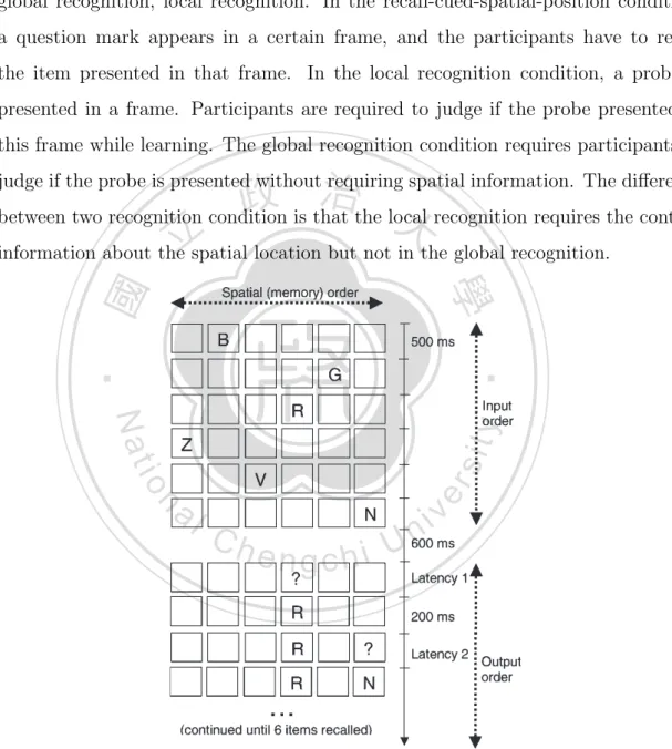
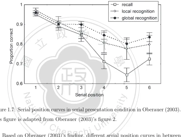
(22) Along with the familiarity process, the recollection is a slow and local matchness process which reaches the specific events (Yonelinas, 2002). The interaction between two processes differs from model to model. The intergration model (eg., STREAK; Rotello, Macmillan, & Reeder, 2004) assumes that the information from familiarity process and recollection intergrate together and the decision is made by the intergrated strength. The dominance model proposes that the old/new response is made by the first process which reaches conclusion (eg., SAC Diana, Reder, Arndt, & Park, 2006).. 1.2. 治. 政 in serial大 Mental process recall and recognition. 立. tasks. ‧ 國. 學. It is not hard to find via looking through the experimental procedure that the. ‧. serial recall and recognition paradigms actually share an almost identical encoding. y. Nat. procedure except the instruction. Both tasks ask participants to remember memory. io. sit. list. Items are presented sequentially on the screen, and the length of memory list. n. al. er. is similar. Also, both tasks share plenty of findings, eg. list length effect, temporal. i n U. v. isolation effect (Morin et al., 2010), and serial postion effect.. Ch. engchi. The serial position effect is that the performance of reponse differs along with the serial position while learning. Both tasks show a similar but different serial position effect. The serial recall task shows a stronger primacy than the recency effect on P C. However the recognition task shows a reversed pattern. An explanation for this difference is that there are different number of responses in two tasks. Serial recall task requires multiple responses, but recognition task only requires one in each trial. Oberauer (2003) examines this hypothesis and other possible sources of the serial effect in both the recall and recognition tasks. He conducted an experiment, in which items are presented in six frames on the screen as shown in Figure 1.6. Two item-presenting sequences are manipulated as: serial and random sequence.. 9.

(23) With the serial presentation sequence, items are presented from left to right in both learning and testing phrases. With the random sequence, items are presented in random order in both phrases. Besides the presentation sequence, participants are instructed with three different retrieval tests applied: recall-cued-spatial-position, global recognition, local recognition. In the recall-cued-spatial-position condition, a question mark appears in a certain frame, and the participants have to recall the item presented in that frame. In the local recognition condition, a probe is presented in a frame. Participants are required to judge if the probe presented in this frame while learning. The global recognition condition requires participants to. 政治大. judge if the probe is presented without requiring spatial information. The difference between two recognition condition is that the local recognition requires the context. 立. information about the spatial location but not in the global recognition.. ‧. ‧ 國. 學. n. er. io. sit. y. Nat. al. Ch. engchi. i n U. v. Figure 1.6: The experiment procedure in Oberauer (2003). Each row represents one display on screen. Presenting sequence is from top to bottom. Items are presented in random order during learning phrase. While testing, a question mark cue shows in a frame. Participant has to recall previous items presented in the frame. This figure is adapted from the Figure 1 in Oberauer (2003).. 10.

(24) The serial presentation condition examines the performance in serial recall and multi–response recognition with/without referencing the contextual information. Serial position curves are shown in Figure 1.7. By adding multiple responses to recognition, both conditions show a greater primacy effect than the recency effect. This supports the hypothesis that the serial position effect difference between serial recall and recognition comes from different numbers of response.. 立. 政治大. ‧. ‧ 國. 學 sit. y. Nat. n. al. er. io. Figure 1.7: Serial position curves in serial presentation condition in Oberauer (2003).. i n U. v. This figure is adapted from Oberauer (2003)’s figure 2.. Ch. engchi. Based on Oberauer (2003)’s finding, different serial position curves in between serial recall and recognition result from that those task have different response processes. The difference disappears after less response process are applied. This leads to an idea that both tasks might have employed the same mental representation underlying. In other words, the same representation in both memory tasks should be conducted with the same encoding process. The only difference between serial recall and recognition task is retrieval process.. 11.

(25) 1.3. Computational modeling. In order to examine the above idea, computational modeling would be the best way to go. The most typical instance about the implication of computational modeling in psychology comes from the seminal study of Nosofsky (1986). Before his study, the identification task and categorization task were usually considered as two separated tasks. That is, the mental processes as well as the mental representation of identification and categorization were thought to be different. In identification, participants are given a list of learned items and asked to identify them. In catego-. 治政 categories. Intuitively, the regime of these two大 tasks are quite similar that implies 立 might be shared between them. Nosofsky (1986) verisome cognitive components. rization, participants are given a list of items and asked to classify them to different. ‧ 國. 學. fied this idea using his categorization model, the GCM (General Context Model). According to this model, the stimuli are encoded as exemplars in our mind which in. ‧. turn are used for categorization. With differential attention allocation on stimulus dimensions, the GCM was evident to be able to account for both the performance. y. Nat. io. sit. in the identification task as well as the categorization task.. n. al. er. The GCM model assumes that an item would be classified to be the category. i n U. v. whose exemplars are much similar to the item. The similarity is transferred from. Ch. engchi. the distance between the items in the psychological space. In addition, the distance on each dimension is weighted by attention weight. For instance, if a dimension is more valid for correct categorization, it will be more attended to, whereas the other dimensions will be less attended to. Therefore, if we regard the identification task as a categorization task with multiple target categories instead of just two or one category in the categorization task, then identification can have a great deal of parts overlapped with categorization. That is, to identify an item is equivalent to examining how similar this item is to the learned exemplar, which is actually itself for successful identification. In the study of Nosofsky (1986), participants were asked to do both the identification and categorization tasks. In the categorization task, all stimuli were composed of two features, one of which was valid for categorization. The GCM was evident 12.

(26) being able to account for the performance in both tasks, with different attention weights on dimensions. That is, for accounting for categorization performance, attention weight on the valid dimension was extremely high, however, for accounting for identification performance, attention weights on both dimensions were almost the same. Thus, this modeling result shows that with the same set of exemplars (i.e., representation), plus different attention weights on stimulus dimensions, the two tasks previously thought different are actually quite similar to each other. This is the instance for the contribution of modeling in psychology. Following Nosofsky (1986)’s methodology, if serial recall and recognition share. 政治大 model which can account for performance of both serial recall and recognition task 立 the same encoding process and representation, there must exist a mathematical. well. For this aim, the present models for serial recall and recognition will be. ‧ 國. 學. discussed to see whether any one of them can actually be the candidate model to examine the hypothesis in this study.. ‧. Previous researches proposed several models which could account for recall and. y. Nat. sit. recognition. For instance, Search of Associative Memory (SAM) model can account. er. io. for recall and recognition in long–term memory. Though many phenomena can. al. v i n Gillund & Shiffrin, 1984).CRetrieving Effectively h e n g c h i U from Memory (REM) model and its extension ARC–REM could also account for recognition and cued recall in long– n. be accounted for, but not the serial position effect (Raaijmakers & Shiffrin, 1981;. term memory. However, the serial position effect could not be simulated (Diller, Nobel, & Shiffrin, 2001; Shiffrin & Steyvers, 1997) still. Therefore, those models concerning performance related to long–term memory should be excluded from the candidate list. In short–term memory, there is one connectionism model (see Burgess & Hitch, 1999) could account for short–term memory serial recall and recognition task. This model is developed based on the association between time and item. However, this model shows smaller primacy effect than the observed data in the serial recall task. In recognition task, the model shows no primacy effect, but recency effect on P C. RT of recognition cannot be simulated either. Therefore, this model is evident. 13.

(27) unable to accommodate both serial recall and recognition performance. SIMPLE (Brown et al., 2002, 2007) is also used to model the result of recognition tasks which use unfamiliar faces as stimulus and fits well to the data in experiments (Hay, Smyth, Hitch, & Horton, 2007). However, SIMPLE model does not adress on the encoding and retrieval processes but the representation of memory. The model that I am looking for is the one which describes the process of encoding and retrieval in enough detail. SIMPLE model does not fit the criterior here. The remaining models in the candidate list can not account both recall and recognition. Therefore, an extension for previous model is needed for previous model. 政治大 Many models had been briefly introduced in the previous section. 立. to account both tasks. The following concern is which model should be extended. In this thesis,. the chosen models are SOB and its successor C-SOB. There are two major reasons. ‧ 國. 學. for selecting those models: the difficulty of modification and examination of the neccessity of context.. ‧. The difficulty of modification to extend SOB and C-SOB into recognition model. y. Nat. sit. is low because of the energy in both models. The energy is one of the core mechanism. er. io. in both SOB model and is defined as the familiarity of incoming item (Farrell &. al. v i n C hof familiarity. SOBUand C-SOB model provide a buildbe defined as the judgement engchi n. Lewandowsky, 2002; Lewandowsky & Farrell, 2008). The recognition process could. in mechanism to determine the familiarity of probe. This reduces the difficulty to extend persist model dramatically.. Second reason for chosing SOB and C-SOB is that the major difference between SOB and C-SOB is the context layer. As mentioned above, SOB model is an ordinal model which encodes order information through signal strength, and serial position is represented through context marker in C-SOB. Hitch, Chiara Fastame, and Flude (2005) used Hebb procedure to examine the underlying mechanism and suggested that the position information plays an important role in serial recall. In other hand, the context information might not be needed in recognition, especially in Sternberg’s task (Corbin & Marquer, 2008, 2009). The necessety of context marker in recognition is examined by comparing the simulation performance between SOB. 14.

(28) and C-SOB.. 立. 政治大. ‧. ‧ 國. 學. n. er. io. sit. y. Nat. al. Ch. engchi. 15. i n U. v.

(29) 2.. Serial–Order in the Box and C-SOB. In this thesis, I assume that serial recall recognition task share the same encoding process and underlying memory representation. In order to verify this assumption, two selected serial order model, Serial-Order in a Box (SOB) and its successor CSOB, are extended to account recognition task. SOB and C-SOB model are connectionist models for short-term serial task. As mentioned in previous chapter, SOB and C-SOB share plenty of features and. 政治大. mechanisms, and the major difference between two models is the way that position information is encoded. SOB assumes that the memory of item is stored in an auto-. 立. association network. The position information is the result of primacy gradient and. ‧ 國. 學. response suppression. Early studied items are encoded with larger encoding strength and result in higher chance to be recalled early in the list (Farrell & Lewandowsky,. ‧. 2002). The successor, C-SOB model, retains the primacy gradient, response suppression, and the auto-association network. A hetro-association connecting between. y. Nat. sit. items and contexts represents the memory of position information. Retrieval is con-. er. io. ducted by using the previous context as retrieval cue. Since that the early context. al. v i n gin of recall(Farrell, 2006;CLewandowsky & Farrell, h e n g c h i U 2008). n. associate with early items, early learned items are easier to be retrieved in the beThe detail of SOB and. C-SOB model are instructed in this section.. 2.1. Serial-Order in a Box model. SOB models the memory trace with an auto-association network. The serial position is coded through the encoding strength. In this auto-association network (W ), the items (v) associates with themselves and are learned with Hebbin rule. One of the most important feature in auto-association network is that the noisy item feeds into network will results in a less noisy item as output. The accuracy and efficiency of deblurring process is influenced by the encoding strength. Deblurring process is an important part in retrieval, see below. 16.

(30) Items are distributed representation and consist with 1 and −1 in both SOB. In SOB model, each items are orthogonal to each other in order to avoid crosstalk in deblurring process. The items are randomly selected from Walsh matrix with 254 dimensionality vectors. In SOB, prior knowledge in the memory trace is carried through pre-train 50 random selected items. pre-training uses Hebbian learning rule as Wk = Wk−1 + ηp vk vkT. (2.1). with very small learning rate (ηp is set to .001). Each chosen items are pre-trained 20 times.. Encoding process. ‧ 國. 學. 2.1.1. 立. 政治大. During encoding phrase, items serial present before participants one by one till list. ‧. running out. SOB model also encodes one item a time till end of list. The same as. (2.2). io. er. Wi = Wi−1 + ηe vi viT .. sit. y. Nat. prelearning, encoding process in SOB is achieved by Hebbian rule as. al. v i n C h between memory which represents the inconsistency e n g c h i U trace and the incoming item. Energy(E) is calculated through n. Unlike prelearning, the encoding strength ηe is not fixed. ηe is determined by energy. ∑ ∑ E = −(ϵ/2) i j wij xi xj , i ̸= j.. (2.3). The wij is the element in the row i and column j of W, and xi and xj represents the element i, j in the vector of incoming item (vi ). The energy calculation is the comparison between the auto-association network W and the outer product of vi with ignoring the diagonal units. The larger E (care the negative in Equation 2.3) indicates the larger inconsistency between memory trace and incoming item. While more items are encoded into memory trace, the energy increases. The encoding strength of current learning item is modulated by the energy through ηe = Ei /ϕe . 17. (2.4).

(31) The more inconsistency between item and memory trace results in the lesser encoding strength of item. For the first item, the inconsistency only comes from the prior in memory trace, thus the encoding strength should be fairly large. The following items receive more inconsistency from the prior and previous encoded items. The encoding strength of later encountered items are smaller than previous. The. 1. 0. 0.8. −100. 0.4. 政治大 −200. 0.6. 立. Energy. Encoding Strength. relationship between energy and encoding strength is illustrated in Figure ??.. −300 −400. 學. ‧ 國. 0.2 −500 0. 1. 2 3 4 5 Serial Position. 6. 1. 2 3 4 5 Serial Position. 6. ‧. Figure 2.1: The energy and encoding strength curve among different serial position. er. io. sit. y. Nat. in SOB.. a. n. 2.1.2. Retrieval lprocess C. hengchi. i n U. v. To retrieve information from memory trace, SOB applies the deblurring process which gradually reduces the noise. The beginning of each item recalling is to randomly generate a vector which consists of +1 and −1. The length of the vector is normalized1 to .0001, and the normalized vector is considered as the seed of deblurring process (v ′ ) and used as the starting point of the deblurring process x(0). x then updates with pre-trained auto-associative network W with x(t + 1) = G[γx(t) + αW x(t)].. (2.5). In the deblurring process, x(t) is fed into W . The input and output of the network are combined with weighted by γ and α. Function G is a non-linear transformation 1. The vector is transferred to having a unit length.. 18.

(32) function, which limits the elements xi in mathbf x within the range between −1 and +1 and is described as.    1    G(x) = xi      −1. if xi > 1 if − 1 ≤ xi ≥ 1 for all xi ∈ x. (2.6). if xi < −1.. The iteration stops when any additional iteration does not change the elements in content or when the iteration times reaches the maximum Imax . Because the initial seed is randomly generated, the most well learned item. 政治大. will be recalled in highest chance. The first item is generally encoded with largest. 立. strength and is the most likely to be retrieved. The retrieved item is then suppressed. ‧ 國. 學. in memory trace with anti-learning. Anti-learning is the same as the learning while encoding but with a negative learning rate ηs (j) which varies based on the energy. ‧. ratio between the energy for the first retrieved item and the energy for the current retrieved ones. The learning rate is calculated by. y. (2.7). er. io. al. −Ej ϕs E1. sit. Nat. ηs (j) =. n. where ϕs is a scalar to adjust the ratio between the first retrieved energy and the. Ch. i n U. v. following energy. The anti-learning rate of the first retrieved item should be 1/ϕs .. engchi. Response suppress plays a important role in SOB, since the first item is the one which most likely to be retrieved. The following items have limited chance to be retrieved in correct sequence without response suppression. However, with response suppression mechanism, the second item becomes the highest activated item after the suppression of first item and could be retrieved in correct order.. 2.2. C-SOB model. In C-SOB model, besides the auto-association network, a fully interconnected hetroassociation network (C) which connects the items and contexts (p) is representing the memory trace. Serial recall task requires participants not only to remember 19.

(33) items, but also remembering specific items in specific orders. Thus the memory should also reflect the connection between items and contexts. Besides the hetro– association network, a fully interconnected auto–association network (W ) between items. The main structure of C-SOB model is displaced in Figure 2.2. Context layer (p) Fully interconnected hetro-associative network (C) Content layer (v) Fully interconnected auto-associative network (W). 學. ‧ 國. 立. 政治大. Figure 2.2: The structure of SOB.. Representation of content. ‧. In C-SOB, the items are 150 dimensionality vectors and consist with 1 and −1. Unlike SOB, the items in C-SOB do not have to be orthogonal. The similarity. y. Nat. sit. between vectors should be determined by experiment material. In most modeling of. er. io. this thesis, the similarity of material is not relatively important. Thus the similarity. al. n. v i n C hand 1 − s probability probability different features e n g c h i U share the same features. In most simulation of this thesis, s is set to 0.5. In results, the average cos value among between material is set to a constant parameter sc . Each content vectors have sc c. c. content vectors is 0.2485. C-SOB model assumes that participants have well known prior knowledge about experiment stimulus. The auto-associative network (W ) is pre-trained with contents representing the prior knowledge. Unlike SOB, items are not orthogonal with each other. There will be cross-talk if W is trained with Hebbian rule. Thus W is pre-trained by Widrow-Hoff learning rule ∆W = ηp vi (vi − oi )T. (2.8). where vi is the item at serial position i and oi is the output when vi put into network W . Prelearning process lasts 300 cycles, and learning rate ηp decreasing with each 20.

(34) cycle k with equation ηp = .03/k. After prelearning, network W could successfully recognize learned items without suffering cross-talk. This serves as an important part in retrieval process.. Representation of context C-SOB model assume the memory trace for serial recall task is the association between items and context. More importantly, each content associates with specific context. C-SOB model assumes context partially changes with events occurring.. 治政 between each context is measured by the Cosine 大 of two context vectors and constraint by the following rule:立 The neighbor contexts are more similar than distant contexts. The relationship. ‧ 國. 學. cos(pi , pl ) = tc(|i−l|) .. (2.9). pi and pl represent the context vectors for item at memory list i and l. The similarity. ‧. between neighbor contexts is represented in tc which is between 0 and 1. If tc equals. y. Nat. to 1, the context markers for every items are exact the same. In other hand, when. al. er. io. sit. tc sets to 0, there are no similarity between context markers.. n. Since the context vectors must fit the constraint of Equation 2.9, some addi-. Ch. i n U. v. tional steps are required. A n×n square matrix (n is the number of items in memory. engchi. list) is generated with  1 t t2c  √ c √  0 1 − t2c tc 1 − t2c  √  0 1 − t2c 0   .. .. .. . . .  0 0 0.  tn−1 c. ... .... tn−2 c. √ n−3. . . . tc ... .... √. 1−.  . t2c  .  1 − t2c    ..  .  √ 1 − t2c .. (2.10). Each column in this matrix fits the rule of Equation 2.9 and is suitable for context vector. However, this rises a problem that the size of matrix changes with set size varied. The size of memory trace (C) must change base on the size of context vector since C is the hetero-association network connecting contexts and contents. In order to keep both network and context in constant size, context vectors are. 21.

(35) several Walsh vector weighted combined with previous matrix. All context vectors have 16 in feature size and 16 in length.. 2.2.1. Encoding process. For every encoded item, memory trace (C) accumulates with association between content and context. The association between item and context is linked with Hebbian rule: ∆Ci = ηe (i)vi pTi .. (2.11). 政治大 position and determined of item i with 立 by the energy . The encoding strength ηe (i) for ith item (vi ) and context (pi ) is varied on serial. ‧ 國. ηe (i) =. 學.  1. , if i = 1.  −ϕe /Ei. (2.12). , if i > 1.. ‧. For the first item in the memory list, the encoding strength ηe (1) is fixed to 1. The. Nat. sit. y. encoding strength for the rest items is determined by their energy Ei and is scaled. io. er. by a scalar ϕe . Here, the energy could be interpreted as the novelty of an item to the participant (Farrell & Lewandowsky, 2004) and is the product of the previous. n. al. Ch. i n U. v. association matrix, item (content vector), and position marker (context vector):. engchi. Ei = −viT Ci−1 pi .. (2.13). Since the energy can be viewed as the novelty, it is true that the encoding strength is sensitive to the novelty of stimulus. The items with more novelty are encoded stronger than those with less novelty. Therefore, from the second item, the encoding strength starts to decrease as the similarity of the encoded and incoming item increases with more features in common to get among the items. This energygated encoding results in the decrease of encoding strength as shown in Figure 2.3. It is important to point out that even the energy in SOB and C-SOB share similar rule in regulating encoding strength, the concepts are different. The energy in SOB is the inconsistency which increases with more encoded items. The energy in 22.

(36) 0. 0.8. −200. 0.6. −400. Energy. Encoding Strength. 1. 0.4. −600. 0.2. 0. −800. 1. 2. 3. 4. 5. 6. −1000. 1. 2. Serial Position. 3. 4. 5. 6. Serial Position. 政治大. Figure 2.3: The energy and encoding strength curve among different serial position in C-SOB.. 立. C-SOB, in the other hand, represents the novelty which decreases with the increasing. ‧ 國. 學. of memorized items. The difference is illustrated in Figure ?? and Figure ??.. ‧. 2.2.2. Recall process in serial recall. sit. y. Nat. io. er. The C-SOB model assumes that the memory trace in the serial recall task is to contain the information about which item in a certain serial position. Hence the. n. al. Ch. i n U. v. retrieval process in the C-SOB model can be understood as a context-based retrieval. engchi. for the content in the memory trace. Due to that the content and context vectors would not be orthogonal, namely noise existed in C, the retrieval of content can be realized as a retrieval plus deblurring process. The retrieving process begins by getting content from the memory trace with the context marker as a retrieval cue. This is achieved by multiplying the context marker of serial position i (pi ) with the memory trace (Ci ) as vi′ = Ci pi .. (2.14). Because the overlapping between position markers, the retrieved content vi′ contains information mainly from the item at serial position i and the items at other positions. In order to reduce the noise, vi′ is processed through the dynamic iterative deblurring process. The deblurring process is the same as SOB except that the initial seed vi′ is not randomly generated but retrieved with context. 23.

(37) After the response is made, the response suppression is applied to the memory trace C. The response suppression is achieved through an anti-learning of the position marker-item association. Anti-learning is the same as the learning while encoding but with a negative learning rate. The equation is defined as ∆Cj = ηs (j)vo,j pTj ,. (2.15). and the learning rate ηs (j) varies based on the energy ratio between the energy for the first retrieved item and that for the following ones. The learning rate is calculated by. −Ej. (2.16) 政治 ϕ E大 is a scalar to adjust the ratio between the first retrieved energy and the 立 ηs (j) =. s. where ϕs. 1. following energy. The anti-learning rate of the first retrieved item should be 1/ϕs .. ‧ 國. 學. The energy of the retrieved item is calculated like the energy while encoding as following:. (2.17). Nat. y. ‧. T Ej = −vo,j Cj−1 pj .. sit. Like SOB, the response suppression process plays a major role in C-SOB. The. er. io. first item in the study list is easiest to retrieve as the first response because of. al. n. v i n encoding strength of theC first h eitem i U the successful rate to retrieve the n gwillc hreduce. its highest encoding strength. However, without response suppression, the higher. second item and the others in the study list through crosstalk. By applying the procedure of response suppression, the first item’s strength gets lower than the second item’s strength after the first item is retrieved, that consequently results in the successful retrieval of following items. Also, response suppression is the source of the recency effect in serial recall. Because the previous items are suppressed, the remaining items have less competence and a larger probability to be recalled.. 24.

(38) 3.. SOB model for recognition. Although subjects have to recall what they have learnt in the serial recall task and recognize which item is previously seen in the recognition task, the leaning process in these two tasks can be pretty much the same. That is, subjects are given a list of digits or consonants to learn one after one in a constant speed, suggesting that what subjects encode in these two tasks can be the same. Therefore, the assumption herein is that the employed representation is not different for these two tasks; only the retrieval process is. In other words, a serial-recall model is. 政治大 examine this assumption, SOB and C-SOB model are chosen as the candidate model 立. presumably able to account for the performance in a recognition task. In order to. for recognition memory for that both models are computational models, providing. ‧ 國. 學. a well-defined architecture which can also trigger the recognition process. Thus, the basic structure of SOB and C-SOB model and the encoding process should. ‧. sit. Nat. modification to the retrieval process is necessary.. y. be remained the same in simulating recognition performance. However, a suitable. er. io. For most recognition models, grounded in no matter the single- or dual-processes. al. v i n similarityC between probe andUthe global hengchi n. view, global matching is regarded as the source for successful recognition, which represents the. states of memory trace. (Hintzman, 1988; Mewhort & Johns, 2005). Familiarity, as another possible source of recognition judgement, is defined the encoding fluency of incoming item and is also an uni-dimension matching process (Jacoby & Kelley, 1992; Wagner & Gabrieli, 1998). In addition to familiarity, the dual-process view endorsers also posit recollection as another source for recognition. Recollection process is relatively slow comparing to familiarity process. Possible recollection process could be recalling every items in the list (Schwartz, Howard, Jing, & Kahana, 2005) or retrieving the context of the probe (Sikström, 2004). Attention often required in recollection process. Contrary to familiarity, the process for recollection is often thought to be slow relatively (Yonelinas, 2002). In traditional Sternberg’s task, both familiarity and recollection. 25.

(39) processes produce the same response for probe. Familiarity process should judge negative probe unfamiliar and familiar with positive probe. Recollection process could successfully retrieval positive probes’ context or recall positive probe. Negative probe is also rejected correctly with recollection process. Since there are no conflict between familiarity and recollection processes, and recollection process happens slower than familiarity. Familiarity process should be able to handle most phenomenon in Sternberg’s task. In this thesis, the recognition process is defined as a consistency- or familiarityjudgement single process for the extension of SOB or C-SOB, respectively. The. 政治大. detail is described in following sections.. 立. ‧ 國. 學. 3.1. The extension of SOB and C-SOB. ‧. A probe is judged as positive (i.e., previously seen) or negative (i.e., previously. y. Nat. unseen) depends on the corresponding consistency or familiarity to an individual. io. sit. it induces. The consistency between probe and memory trace could be measured. n. al. er. through the energy computation in SOB model. In the other hand, the energy in. i n U. v. C-SOB represents the familiarity which could be a source of old/new judgement.. Ch. engchi. Thus, both models compute the energy of probe to make a recognition response. Also, the induced energy for a probe needs to exceed a criterion value for making a positive response. The distance of the energy to the criterion can be regarded as the difficulty to make a positive response, as this distance can be converted to reaction time; the larger the distance, the longer the RT is. In this section, the details of these modifications for SOB model are introduced.. 26.

(40) 3.1.1. Measuring energy of probe. SOB model SOB model assumes that the memory traces are self-associated items. The energy of incoming item is the difference between matrix of memory traces and the outer product of incoming item, as seen in Equation 3.1. The larger the difference, the larger the energy is. The consistency between probe and memory traces could be measured in the same way. The more consist between probe and memory traces, the smaller the difference is, and results in smaller energy of probe. The consistency. 政治大. of probe is defined as the energy of probe in SOB mode.. 立. ‧ 國. 學. ∑ ∑ E = −(ϵ/2) i j wij xi xj , i ̸= j.. (3.1). ‧. Since that the negative probes are never presented while learning, the source of consistency should only comes from the prior, and results in a large inconsistency. y. Nat. sit. and energy. Positive probes, in the other hand, are encoded in memory trace while. al. er. io. learning, should have smaller energy. Also, the increasing of set size decreases the. n. consistency of probe and results in larger energy, as shown in Figure 3.1. 4. x 10 0. Ch. engchi. i n U. v. Energy. −0.5 Positive probe Negative probe. −1 −1.5 −2 −2.5. 3. 4. 5. 6. Set size. Figure 3.1: The energy of positive probe and negative probe among different set sizes in SOB. However, the consistency of positive probe comes from both prior knowledge and learning, and the encoding strength varied the consistency. The encoding 27.

(41) strength, as a result of energy-gated encoding, shows the primacy gradient that the strength decreases along with serial position. The consistency of positive probe shows only primacy gradient as Figure 3.2. 4. x 10. −0.5. Energy. −1. −1.5. −2. −2.5. −3. 1. 立. 政治大 2. 3 4 Serial position. 5. 6. ‧ 國. 學. Figure 3.2: The energy position curve among different serial position.. ‧. C-SOB model. y. Nat. sit. Unlike a straightforward way to measuring the energy of probe in SOB, C-SOB. er. io. model requires more works. In C-SOB model, the memory traces of learned items. al. are stored in the associations between the context and content layers. The system. n. v i n energy for an input item C can be viewed as the resonance of the memory traces to hengchi U the current item. Presumably, the resonance to an item is larger if it is more similar. to the previously learned items in the memory traces. Due to that the energy value is always negative as seen in Equation 3.2, the larger the resonance, the smaller the energy is. Applying this logic to the recognition of an item, it is straightforward to expect that a probe (i.e., the item presented in the recognition stage) would induce a smaller energy if it is similar to the items in the memory traces and vice versa. In other words, this probe is familiar to the system. Thus, the familiarity to a probe can be defined as the energy of system induced by it.. Ei = −viT Ci−1 pi .. (3.2). In C-SOB model, the energy is the product of the content vector (vi ) of an 28.

(42) item i, the context vector (pi ) for the item i, and the memory trace matrix (Ci−1 ). Parallel to this computation, the energy in the recognition task is the product of the content vector of a probe (vp ), the context vector for the probe (pp ), and the memory trace matrix (Ci−1 ). This turns Equation 3.2 into Equation 3.3. Ep = −vpt Cpp .. (3.3). The context vector for the probe pp is created using the same algorithm in C-SOB model, with the correlation to the context vector of the learned item pi , which is defined as (3.4) 政治大 ≤ 1 and 0 ≤ t ≤ 1 respectively denote the correlation between 立 cos(pi , pp ) = tp tn−i c ,. where 0 ≤ tc. p. two adjacent context vectors and the correlation between the context vector of the. ‧ 國. 學. last item and that of the probe, with set size = n. The energy of positive probes and negative probes among different set size are shown in Figure 3.3 According to. ‧. Equation 3.4, the closer the item to the probe, the higher the correlation between. y. Nat. them is. During the encoding stage, the energy decreases as encoding proceeds.. io. sit. However, this is not necessary the case for recognizing the probe. For the positive. n. al. er. probe, the energy actually varies along the position of the probe in the learning. i n U. v. list. Figure 3.4 shows that the energy is the largest for the middle position and. Ch. engchi. the smallest for the first and the last position when set size is greater than 3. As mentioned before, the larger the energy, the less familiar the system is with the probe. Therefore, this reversed U curve indicates that the very first and very last items are most likely to be recognized and the middle items are relatively hard to be recognized; namely the primacy and recency effect in recognition memory. The mathematical proof is provided as follow. First, the energy for a probe is computed by Equation 3.3. With the set size = n, given the memory trace Cn is Cn =. n ∑ i=1. 29. ηi vi pTi ,. (3.5).

(43) −400. −600. Energy. −800. −1,000. −1,200. −1,400. −1,600. 立. 3. 政治大 4. Positive probe Negative probe. 5. 6. Setsize. ‧ 國. 學. Figure 3.3: The energy of positive probe and negative probe among different set sizes in C-SOB.. ‧ er. io. sit. y. Nat. n. al. Ch. −900. engchi. i n U. v. Setsize 3 Setsize 4 Setsize 5 Setsize 6. −1000. Energy. −1100. −1200. −1300. −1400. −1500. 1. 2. 3. 4. 5. 6. Serial Position. Figure 3.4: The energy position curve among different set size and serial position.. 30.

(44) Equation 3.3 will then become Ep =. −vpT (. =−. n ∑. ηi vi pTi )pp. i=1 n ∑. ηi (vpT. (3.6) ·. vi )(pTi. · pp ).. i=1. Because the length of pi and pp are equal to 16, given that the product of two vector lengths equals the inner product between these two vectors divided by the cosine value between them cos(a, b) = √. a·b √ a·a b·b. (3.7). 政治大 ∑. and Equation 3.4, the energy of probe could be reform as. 立E. p. n. =−. ηi (vpT · vi )[162 cos(pi , pp )]. n ∑. ηi (vpT · vi )(tp tn−i c ). i=1 n ∑. = −162 tp. (3.8). ‧. ‧ 國. = −162. 學. i=1. ηi (vpT · vi )(tn−i c ).. i=1. y. Nat. sit. The similarity on context between the probe and the learning item i is tn−i c , which. er. io. decays along the distance to the last item from the learning item. Although vpT · vi. al. n. v i n C h for the first item, learning item, with the largest e n g c h i U as shown in Figure 2.3. Together. is the same for the probe being on any position, ηi decays along the position of the. with the similarity on context between item and probe, the energy would be the most negative for the probe being on the earlier or the latter position in the learning list and would be the least negative for the probe being on the middle position. This is the reason for a reserved U profile of the energy for a positive probe. One thing to note is that although tp does not change the shape of the energy curve, it might be sensitive to the consistency of the context for the stimulus between the encoding and retrieval stages, larger for the consistent case and smaller for the inconsistent case. For the simulations in this study, tp is set to be constant. The energy Ep for the negative probe must be larger than that for the positive probe, as exactly one product of vpT · vi is larger in the case for the positive probe than in the case for the negative probe. 31.

(45) 3.1.2. Placing decision criterion of energy. The energy is regarded the source for determining a probe as old or new. As Ep should be larger for a negative probe than a positive one, the recognition can be done by simply comparing the energy induced for the probe to a criterion. If the energy is larger than the criterion, the probe is regarded as new and vice versa. Both positive and negative probes could get their energy through Equation 3.3. In order to simulate old/new response, a decision criterion is placed to judge their consistency/familiarity. If probe’s energy is bigger than criterion (remember the neg-. 政治大. ative in Equation 3.1 and Equation 3.3), probe is unfamiliar enough and considered. 立. as new item.. ‧ 國. 學. There are several possible ways to place criterion. The simple way to do so is held the criterion constant among all set sizes. Different set sizes sharing the same. ‧. decision criterion. Another method is assuming decision criterion change through. Nat. (3.9). er. io. al. τn = τs × n + τi .. sit. This could be write as a linear function as following:. y. different set sizes. In this method, I assume criterion change linearly with set sizes.. n. v i n τ is the decision criterion the slope of linear function, and τ is Cofhset size n. τ is U i e h n c which criterion is constant, τ is simply the intercept. In fact, for simplified g version n. s. i. s. set to zero. The constant criterion model is a restricted version of linear changed model. Both methods are shown in Figure 3.5. After placing decision criterion, strength of presence/absence is determined by the distance between energy of probe and criterion. If the energy of probe is closer to criterion, it is harder to make old/new judgement than the distance is longer. Response tendency is used to simulate the quickness or accuracy of response. Response tendency is the reciprocal of signal strength and is calculated differently from positive and negative probe. For positive probe, the response tendency is calculated with Response tendency = −. 32. 1 . Ep − τn. (3.10).

(46) −400. −600. −600. −800. −800. Energy. Energy. −400. −1,000. −1,200. −1,200. −1,400. −1,600. −1,000. −1,400. Positive probe Negative probe Decision criterion 3. 4. 5. −1,600. 6. Positive probe Negative probe Decision criterion 3. 4. Setsize. 5. 6. Setsize. Figure 3.5: Two different method to place decision criterion. Left figure is the constant criterion. Right figure is the linear criterion. Dash–dot line indicates the. 政治大 negative probe, respectively. Errorbar is one standard deviation of mean energy. 立. decision criterion. Solid line and dot line are the mean energy of positive probe and. ‧ 國. 學. The negative probe response tendency is calculated by Response tendency =. (3.11). ‧. 1 . Ep − τn. Unlike signal strength, response tendency goes the same direction as RT . The higher. Nat. sit er. io. a. iv l Cmethod and results Simulation n U n. 3.2. y. response tendency should indicate longer RT and lower P C, and vice versa.. hengchi. Combining SOB/C-SOB and two criteria, four models are simulate the basic findings in recognition task in order to select suitable model for future simulation. The selected basic finding is the list length effect and the serial position effect. The parameters will influence simulation results are shown in Table ??. The encoding strength of prior knowledge etap is fixed to .0001 in SOB. In C-SOB model, the similarity between the last context of item and the context of probe tr is a scalar and fixed to .8. Also, similarity between items (sc ) should be determined by experiment materials and is fixed to .5. The value of other parameters are shown in Table ??. The serial position effect of response tendency are displayed in Figure 3.6. There is no obvious difference between two criteria, but the pattern in SOB and C-SOB are quite distinct. C-SOB model capture the pattern of serial position effect with 33.

(47) Table 3.1: The best fitting parameters for both model. Models. SOB ϕe. C-SOB. τi. τs. ϕe. tc. τi. τs. Constant 600. -8500. 0. 240. .75. -920. 0. Linear. -15000. 1150. 240. .72. -1150. 55. 600. lower primacy and stronger recency effect. However, the serial position effect in SOB model shows only primacy but recency effect. The same pattern in the energy also shows on response tendency.. 政治大 in Figure 3.7. There is not much difference between SOB and C-SOB. Though both 立. The mean response tendency of positive probe and negative probe are shown. criteria perform well in positive probe. Constant criterion model fail to capture the. ‧ 國. 學. second law that Sternberg purposed (Sternberg, 1966, 1969). The slope of positive probe and negative probe is not equal. Only linear criterion model could simulate. ‧. this finding.. sit. y. Nat. er. Discussion. io. 3.3. al. n. v i n C of simulation results, While considering the trend h e n g c h i U linear criterion captures the pat-. tern of mean reaction time better than constant criterion. Though both criteria show the pattern of linear increasing of positive probe. The slope of positive probe and negative probe is not equal in the simulation of constant criterion but linear. This approves the linear criterion. C-SOB capture the trend of serial position effect. Simulation shows an inverse U shape response tendency curve with smaller primacy and larger recency effect. The tunning point of primacy and recency effect is at about second serial position. The response tendency of last item is about the same regarding set size. In the other hand, SOB model failed to simulate the serial position effect. SOB model shows only primacy effect but recency. Also, the response tendency in SOB concaves up, but the real data shows the pattern of concaving down. The simulation on serial position 34.

(48) −3. x 10. 3.5. 2.5. 政治大. 2 1.5. 立. 1. x 10. 1.5. Response Tendency. Response Tendency. −3. Set size 3 Set size 4 Set size 5 Set size 6. 3. 1. set size 3 set size 4 set size 5 set size 6. 0.5. 0.002 0. 1. 2. 3 4 Serial position. 5. 6. x 10. 10 set size 3 set size 4 set size 5 set size 6. al. 9. n. 0.004. 2. −3. io. 0.006. 1. Ch. 3 4 Serial position. y. 8 7 6 5. i n U. 4. engchi 5. 6. set size 3 set size 4 set size 5 set size 6. sit. 0.008. 0. 6. er. 0.01. 5. 11. Nat. Response tendency. 0.012. 3 4 Serial position. ‧. 0.014. 2. Response tendency. 1. 學. 0. ‧ 國. 0.5. v. 3 2. 1. 2. 3 4 Serial position. 5. 6. Figure 3.6: The response tendency among serial position of four models. The upper left and figures show the response tendency of SOB with constant and linear criterion, respectively. The button left and right figures show the response tendency for constant and linear criterion in C-SOB.. 35.