Vertex fault tolerance for edge-bipancyclicity of hypercube

(1)

Vertex fault tolerance for edge-bipancyclicity of

hypercube

Chun-Nan Hung

Department of Computer Science and Information Engineering Da-Yet University, Changhua,

Taiwan 51505, R.O.C Email:[email protected]

Yu-Chun Lin

Department of Computer Science and Information Engineering Da-Yet University, Changhua,

Taiwan 51505, R.O.C Email:[email protected]

Abstract—A bipartite graph G = (V, E)

edge-bipancyclic if every edge lies on the cycles of every even length from 4 to |V |. Let Qn = (Vb∪ Vw, E) be an

n-dimensional hypercube where Vb and Vw are the sets of

black and white vertices, respectively. Let Fb(resp. Fw) be

the set of black (resp. white) faulty vertices. In this paper, we will show that Qn− Fb − Fw is edge-bipancyclic if |Fb|, |Fw| ≤ b

n₋₁ 4 c.

Index Terms—hypercube, edge-bipancyclic, bipartite

graph, vertices fault-tolerance

I. INTRODUCTION

The hypercube network is one of the most popular interconnection networks. It has many attractive properties, such as regularity, symmetry, small de-gree and diameter, maximum fault tolerance, easy routing algorithms.

An interconnection network is usually repre-sented by a graph where vertices represent proces-sors and edges represent links between procesproces-sors. Let G = (Vb∪ Vw, E) be a bipartite graph where Vb

and Vw are two disjoint vertex sets such that each

edge of E consists of one vertex from each set. Let d(u, v) be the distance of the vertices u and v. A

bi-partite graphG = (Vb∪ Vw, E) is Hamiltonian lace-able if there exists a Hamiltonian path between x, y

for any x ∈ Vb, y ∈ Vw. The graphG = (Vb∪Vw, E)

is hyper-Hamiltonian laceable if ∀v ∈ Vb(resp. Vw),

there exists a Hamiltonian path ofG − {v} between

each pair of vertices ofVw(resp.Vb). In [13], Tsai et

al. proved that Qn− Fe is Hamiltonian laceable for

Fe ⊂ E(Qn), |Fe| ≤ n − 2 and hyper-Hamiltonian

laceable for Fe ⊂ E(Qn), |Fe| ≤ n − 3. A bipartite

graph G = (V, E) is edge-bipancyclic if every edge

of E lies on cycles of every even length from 4 to |V |. In [8], Li et al. proved that Qn− Fe is

edge-bipancyclic for Fe ⊂ E(Qn), |Fe| ≤ n − 2.

There is little literature about general vertex fault tolerant Hamiltonian properties of hypercube Qn =

(Vb ∪ Vw, E). Some literatures concern embedding

fault-free cycles or paths for hypercube with faulty vertices. The upper bound of longest fault-free cycle of Qn− Fv is 2n− 2f where Fv is the faulty set of

vertices ofQn andf = max{|Fv∩Vw|, |Fv∩Vb|}. In

[2], [4], [10], [12], the authors showed that a fault-free cycle of length2n_−2f

v can be constructed with

fv faulty vertices. In [5], [14], the authors showed

that every edge in Qn− Fv − Fe lies on cycles of

every even length from 4 to 2n_{− 2|F}

v| if |Fv| +

|Fe| ≤ n−2. When all faulty vertices are in the same

partite set, this result is the vertices fault tolerance for edge-bipancyclicity ofQn. However, there exist

longer cycles when both partite vertex sets contain some faulty vertices.

In [1], Caha et al. proposed the multiple span-ning paths problem for hypercube. Let si, ti, for

1 ≤ i ≤ k, be vertices of Qn. The {si, ti}ki=1 is a connectable family if there exists k spanning paths P (si, ti) of Qn for 1 ≤ i ≤ k. The {si, ti}ki=1 is balanced if it has the same number of vertices in

each partite set. Caha showed that every balanced family {si, ti}ni=1 is connectable in Q2n if d(si, ti)

is odd for 1 ≤ i ≤ n. Caha also showed that

every balanced family {si, ti}ni=1 is connectable

in Q6n. In [7], Hung et al. investigated the fault

(2)

Let the family {si, ti}Fb,KbFw,Kw of Qn be the vertex set

Kb ∪ Kw = {si, ti| for 1 ≤ i ≤ (|Kb| + |Kw|)/2}

of Qn − Fb − Fw. The family {si, ti}Fb,KbFw,Kw is

balanced if 2|Fb| + |Kb| = 2|Fw| + |Kw|. The

family {si, ti}Fb,KbFw,Kw is connectable if there exit

(|Kb| + |Kw|)/2 spanning disjoint paths P (si, ti)

for 1 ≤ i ≤ (|Kb| + |Kw|)/2 of Qn − Fb − Fw.

The authors showed that every family {si, ti}Fb,KbFw,Kw

ofQnis connectable if|Kb|+|Kw|+|Fb|+|Fw| ≤ n

and 4|Fb| + 2|Kb| = 4|Fw| + 2|Kw| ≤ n + 1.

In this paper, we incorporate the adjacently faulty vertices into the vertex fault tolerance of multiple spanning paths of hypercube. Let {si, ti}Fb,KbFw,Kw be

a family of G = (Vb ∪ Vw, E) − Fa where Kb ∪

Kw = {si, ti|1 ≤ i ≤ (|Kb| + |Kw|)/2} is the set

of fault-free vertices, Fa is the set of |Fa| pairs of

adjacently faulty vertices, Fb ⊂ Vb andFw ⊂ Vw are

sets of faulty vertices. In this paper, we will show that every family{si, ti}Fb,KbFw,Kw of hypercubeQn−Fa

is connectable if|Fb|+|Fw|+|Kb|+|Kw|+|Fa| ≤ n,

4|Fb| + 2|Kb| + |Fa| = 4|Fw| + 2|Kw| + |Fa| ≤ n + 1,

for n ≥ 3. Applying this result, we can obtain that Qn − Fb − Fw is edge-bipancyclic if |Fb|, |Fw| ≤

bn−1 4 c.

The rest of this paper is organized as follows. In Section 2, we introduce some important defini-tions and lemmas. Section 3 shows the vertex fault tolerance for multiple spanning paths. The vertex fault-tolerance for edge-bipancyclicity is introduced in Section 4. We finally give some conclusion in Section 5.

II. PRELIMINARIES

An n-dimensional hypercube Qn = (Vb∪ Vw, E)

is a bipartite graph whose vertices are labeled by distinct n-bit binary strings. Two vertices are linked

by an edge if and only if their labels differ exactly in one bit. The hypercube Qn can be constructed

recursively as Qn = Qn−1× K2. We can partition

Qn as two subgraphs Q0_n−1 and Q1_n−1 by choosing

any one bit of binary string.

We call the Vb black vertex set andVw white

ver-tex set. LetVbj andVwj be the black and white vertex

set of Qj_n−1 for j = 0, 1. And let Vj _{= V}j

b ∪ Vwj for

j = 0, 1. Thus, Vb = Vb0∪ Vb1, Vw = Vw0 ∪ Vw1, V =

Vb∪ Vw = V0∪ V1.

Let Fb be the set of black faulty vertices and Fw

be the set of white faulty vertices of Qn. Similarly,

we also use F_bj and Fj

w to denote the black and

white faulty vertex set of Qjn−1, respectively, for

j = 0, 1. Thus, Fb = Fb0∪ Fb1, Fw = Fw0∪ Fw1, F0 =

F0

b ∪ Fw0, F1 = Fb1∪ Fw1.

Let Fa be the set of adjacently faulty vertices

of Qn. Similarly, we also use Faj to denote the

adjacently faulty vertex set of Qjn−1, respectively,

forj = 0, 1. Thus, Fa = Fa0∪ Fa1. We further define

F = Fb∪ Fw∪ Fa.

Let Kb andKw be the black and white fault-free

vertex set. LetK = Kb∪Kw = {si, ti|1 ≤ i ≤ |K|₂ }.

And letK_bj = Kb∩Vj, Kwj = Kw∩Vj, for j = 0, 1.

Let φ(v) be a vertex of Vi _{for every} _{v ∈ V}j

such that (v, φ(v)) ∈ E and {i, j} = {0, 1}. Let X = {x1, x2, · · · , xk} be a vertex subset of Qin−1

for i = 0, 1. We define the free neighbor set of X

is N(X) = {uj|(xj, uj) ∈ E(Qin−1) and φ(uj) /∈

(F ∪ K) for 1 ≤ j ≤ k, i = 0, 1}. Let φ(X) = {φ(v)|v ∈ X} be a vertex subset of Vj _for _{X ⊂ V}i

for {i, j} = {0, 1}.

We need some previous results for our proofs. The following lemma is proposed in [6].

Lemma 1: The graphQnisf -adjacency (n − 2 −

f ) edges Hamiltonian for 0 ≤ f ≤ (n − 2), f

-adjacency (n−2−f ) edges Hamiltonian laceable for 0 ≤ f ≤ (n − 3), and f -adjacency (n − 3 − f ) edges

hyper-Hamiltonian laceable for 0 ≤ f ≤ (n − 3).

A bipartite graph G = (Vb∪ Vw, E) has property 2H if for any s1, s2 ∈ Vb and t1, t2 ∈ Vw there exist

two spanning disjoint paths P (s1, t1) and P (s2, t2)

of G. Su et al. proved the following lemma in [11].

Lemma 2: The graph Qn− Fa− Fe has property

2H whereFais the set of|Fa| pairs adjacently faulty

vertices and Fe is the set of faulty edges and 0 ≤

|Fa| + |Fe| ≤ n − 3.

III. VERTEX FAULT TOLERANCE FOR MULTIPLE SPANNING PATHS IN HYPERCUBE

In this section, we will prove the vertex fault tolerance for multiple spanning disjoint paths of

(3)

hypercube. The following lemma is the proof for some property for Q4.

Lemma 3: Let s1, t1 ∈ Vw ands2, t2 ∈ Vb be two

pairs of fault-free vertices. there exist two spanning disjoint paths P (s1, t1) and P (s2, t2) of Q4.

Proof. By symmetry of hypercube, we can arrange

s1 in Q03 andt1 in Q13. We will prove this lemma in

the following cases.

Case 1. s2 and t2 in the same subcube.

Without loss of generality, we can assume thats2, t2

are in Q1

3. We can construct a Hamiltonian path

hs2

P(s2,t2)

−→ t2, x

P(x,t1)

−→ t1i of Q13. We can also

construct a Hamiltonian path P (s1, φ(x)) of Q03.

Thus, P (s2, t2) and hs1

P(s1,φ(x))

−→ φ(x), x P−→ t(x,t1) 1i

are two spanning disjoint paths of Q4.

Case 2. s2 and t2 in different subcubes.

Without loss of generality, we can assume that s2 ∈

Q1

3 and t2 ∈ Q03. We can construct a Hamiltonian

path hs1

P(s1,x1)

−→ x1, x2

P(x2,t2)

−→ t2i of Q03 for x1 ∈ Vw0

and{φ(x1), φ(x2)}∩{s2, t1} = ∅. Applying Lemma

2, we can further construct two spanning disjoint paths P (φ(x1), t1) and P (s2, φ(x2)) of Q13. Thus,

hs1 P(s1,x1) −→ x1, φ(x1) P(φ(x1),t1) −→ t1i and hs2 P(s2,φ(x2)) −→ φ(x2), x2 P(x2,t2)

−→ t2i are two spanning disjoint paths

of Q4. 2

Theorem 1: Every family {si, ti}Fb,KbFw,Kw of

hyper-cubeQnis connectable if|Fb|+|Fw|+|Kb|+|Kw|+

|Fa| ≤ n, 4|Fb| + 2|Kb| + |Fa| = 4|Fw| + 2|Kw| +

|Fa| ≤ n + 1, |Fa| ≤ n − 3 for n ≥ 3.

Proof: We will prove this theorem by induction on

n. When |Fb|+|Fw|+|Kb|+|Kw|+|Fa| < n, 4|Fb|+

2|Kb| + |Fa| = 4|Fw| + 2|Kw| + |Fa| < n + 1, |Fa| <

n − 3, the proof of Qn is the same as the proof of

Qn−1. Thus, we only need to prove that at lest one of

the conditions|Fb| + |Fw| + |Kb| + |Kw| + |Fa| = n,

4|Fb| + 2|Kb| + |Fa| = 4|Fw| + 2|Kw| + |Fa| =

n + 1, |Fa| = n − 3 holds.

Applying Lemma 1, we can obtain that Qn− Fa is

Hamiltonian laceable and hyper-Hamiltonian lace-able for |Fa| = n − 3. Thus, this theorem is true for

|Fa| = n − 3. It is true for n = 3.

We consider the case for n = 4. Applying Lemma

2, we can also obtain that Q4 has the property 2H.

Applying Lemma 3, we can construct two spanning disjoint pathsP (s1, t1) and P (s2, t2) of Q4forKb =

{s1, t1}, Kw = {s2, t2}. Thus, this theorem is true

for n = 4.

We will prove the induction step for |Fa| ≤ n − 4

and n ≥ 5 with the following cases. By the

symmetry of hypercube, we can assume that every pair of adjacently vertices is either in Q0

n−1 or

Q1

n−1. We draw Q12 in figures of some cases for

illustration.

Case 1: n − |Fa| is even.

When |Fb| + |Fw| ≥ 1, the proof of this case is

the same as the case of Qn−1. Thus, we only need

to prove this case for |Fb| = |Fw| = 0. We can

infer that |Kb| + |Kw| + |Fa| = n. Without loss of

generality, we can assume that |F0

a| ≥ |Fa1|.

Case 1.1: |Fa| = 0.

Without loss of generality, we can assume that

|K0_{| ≥ |K}1_{| ≥ 1 and |K}0

b| ≥ |Kw0| ≥ 1.

Case 1.1.1: |K1_{| = 1.}

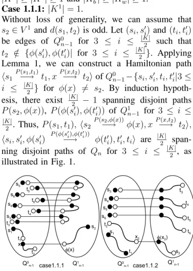
s2 ∈ V1 and d(s1, t2) is odd. Let (si, s0i) and (ti, t0i)

be edges of Q0 n−1 for 3 ≤ i ≤ |K| 2 such that t2 ∈ {φ(s/ 0i), φ(t0i)| for 3 ≤ i ≤ |K| 2 }. Applying

Lemma 1, we can construct a Hamiltonian path

hs1

P(s1,t1)

−→ t1, x P(x,t2)

−→ t2i of Q0n−1−{si, s0i, ti, t0i|3 ≤

i ≤ |K|₂ } for φ(x) 6= s2. By induction

hypoth-esis, there exist |K|₂ − 1 spanning disjoint paths P (s2, φ(x)), P (φ(s0i), φ(t0i)) of Q1n−1 for 3 ≤ i ≤ |K| 2 . Thus, P (s1, t1), hs2 P(s2,φ(x)) −→ φ(x), xP−→ t(x,t2) 2i, hsi, s0i, φ(s0i) P(φ(s0 i),φ(t0i)) −→ φ(t0 i), t0i, tii are |K|₂

span-ning disjoint paths of Qn for 3 ≤ i ≤ |K|₂ , as

illustrated in Fig. 1.

Fig. 1. Illustration of Case 1.1.1 and Case 1.1.2

Case 1.1.2: |K1_{| ≥ 2 and s}

i, ti ∈ K0 for some

(4)

s1, t1 ∈ Q0n−1. Let t2 be vertex of Q0n−1 with

{s1, t1, t2} 6⊂ Kb and {s1, t1, t2} 6⊂ Kw. Without

loss of generality, we can assume that s1, t1 ∈

Kb, t2 ∈ Kw. Let x2 ∈ Kw0 for φ(x2) /∈ K1. Let

K0 _{= K}0_{− {s}

1, t1, t2}, N(K0) be the free neighbor

set of K0_{. Applying Lemma 3, we can construct}

two spanning disjoint paths P (s1, t1) and P (x2, t2)

of Q0

n−1− K0 − N(K0). By induction hypothesis,

there exist |K|₂ − 1 spanning disjoint paths between (φ(N(K0)) ∪ K1∪ {φ(x2)}) of Q1n−1. Therefore, we

can construct |K|₂ spanning disjoint paths between

Kb∪ Kw of Qn as illustrated in Fig. 1.

Case 1.1.3: si andti in different subcubes for every

1 ≤ i ≤ |K|₂ .

Without loss of generality, we can that si ∈ Q0n−1,

andti ∈ Q1n−1for1 ≤ i ≤ |K|

2 . Suppose thatd(si, ti)

is odd for some 1 ≤ i ≤ |K|₂ . Without loss of gener-ality, we can assume thatd(s1, t1) is odd. Let (t01, t1)

be an edge of Q1

n−1 fort01, φ(t01) /∈ K. Let (si, s0i) be

edges of Q0

n−1 for s0i, φ(s0i) /∈ (K ∪ {t01, φ(t01)}) for

2 ≤ i ≤ |K|₂ . Applying Lemma 1, we can construct a Hamiltonian pathP (s1, φ(t01)) of Q0n−1−{si, s0i|2 ≤

i ≤ |K|₂ }. By the induction hypothesis, there

ex-ist |K|₂ − 1 spanning disjoint paths P (φ(s0

i), ti) of

Q1

n−1 − {t1, t01}. Therefore, we can construct |K|

2

spanning disjoint paths hs1

P(s1,φ(t0 1)) −→ φ(t0 1), t01, t1i, hsi, s0i, φ(s0i) P(φ(s0 i),t0i) −→ t0 ii of Qn for 2 ≤ i ≤ |K|₂ , as illustrated in Fig. 2.

Fig. 2. Illustration of Case 1.1.3

Suppose that d(si, ti) is even for every 1 ≤ i ≤ |K|₂ .

s1 ∈ Kb and s2 ∈ Kw. Let (t01, t1), (t02, t2) be edges of Q1 n−1 for t02, t02, φ(t01), φ(t02) /∈ K. Let (si, s0i) be edges of Q0n−1 for s0i, φ(s0i) /∈ (K ∪ {t0 1, t02, φ(t01), φ(t02)}), for 3 ≤ i ≤ |K| 2 . By induction

hypothesis, there exist two spanning disjoint paths

P (s1, φ(t01)) and P (s2, φ(t20)) of Q0n−1− {si, s0i|3 ≤

i ≤ |K|₂ }. By induction hypothesis, there also

exist |K|₂ − 2 spanning disjoint paths P (φ(s0

i), ti) of

Q1

n−1− {t1, t01, t2, t02}. Therefore, we can construct |K|

2 spanning disjoint pathshsi

P(si,φ(t0 i)) −→ φ(t0 i), t0i, tii, hsj, s0j, φ(s0j) P(φ(s0 j),t0j) −→ t0 ji of Qn for 1 ≤ i ≤ 2, 3 ≤ j ≤ |K|₂ , as illustrated in Fig. 2(b). Case 1.2: |Fa| ≥ 1 and |Fa1| = 0. Case 1.2.1: |K1_{| = 0.}

We can infer that |Kb| ≥ 2 and |Kw| ≥ 2 since

|Fb| = |Fw| = 0 and |Fa| ≤ n − 4. Without

loss of generality, we can assume that s1, t1 ∈ Vb

and s2, t2 ∈ Vw. Let (si, s0i), (t0i, ti) be edges of

Q0

n−1 for s0i, t0i ∈ (K ∪ F ) for 3 ≤ i ≤/ |K|

2 .

Applying Lemma 2, we can construct two span-ning disjoint paths hs1

P(s1,s0 1) −→ s0 1, t02 P(t0 2,t2) −→ t2i and hs2 P(s2,s0 2) −→ s0 2, t01 P(t0 1,t1) −→ t1i of Q0n−1 − Fa0 − {si, s0i, ti, t0i|3 ≤ i ≤ |K| 2 }. By induction

hypoth-esis, we can construct |K|₂ spanning disjoint paths

P (φ(s0 i), φ(t0i)) of Q1n−1 for 1 ≤ i ≤ |K| 2 . Therefore, hsi P(si,s0 i) −→ s0 i, φ(s0i) P(φ(s0 i),φ(t0i)) −→ φ(t0 i), t0i, P(t0 i,ti) −→ tii, hsj, s0j, φ(s0j) P(φ(s0 j),φ(t0j)) −→ φ(t0 j), t0j, tji are |K|₂

span-ning disjoint paths of Qn− Fa for 1 ≤ i ≤ 2, 3 ≤

j ≤ |K|₂ , as illustrated in Fig. 3.

Case 1.2.2: |K0_{| = 0.}

By induction hypothesis,we can construct |K|₂ span-ning disjoint paths betweenKb∪Kw ofQ1_n−1.

With-out loss of generality, we can denote these paths as

hs1, P(s1,u)

(5)

F0

a, 2 ≤ i ≤ |K|

2 . Applying Lemma 1, we

can construct a Hamiltonian path P (φ(u), φ(v)) of Q0

n−1− Fa0. Therefore, hs1, P(s1,u)

−→ u, φ(u)P(φ(u),φ(v))−→ φ(v), v P−→(v,t1) t1i, P (si, ti) are the |K|₂ spanning

disjoint paths of Qn − Fa for 2 ≤ i ≤ |K|₂ , as

Case 1.2.3: |K0_{| = 1.}

s1 ∈ Vb0. Let x ∈ Vw0 for x, φ(x) /∈ (K ∪ F ).

Applying Lemma 1, we can construct a Hamiltonian path P (s1, x) of Q0n−1− Fa0. By induction

hypoth-esis, we can construct |K|₂ spanning disjoint paths

P (φ(x), t1), P (si, ti) of Q1n−1 for 2 ≤ i ≤ |K|2 .

Therefore, hs1, P(s1,x)

−→ x, φ(x) P(φ(x),t1)−→ t1i, P (si, ti)

are the |K|₂ spanning disjoint paths of Qn− Fa, as

Case 1.2.4: |K1_{| = 1.}

Without loss of generality, we can assume that t1 ∈

V0

w. Since |Vb| ≥ 2, |Vw| ≥ 2, we can choose two

black vertices and one white vertex of K0_{. Without}

loss of generality, we can assume that s1, t2 ∈

Vb, s2 ∈ Vw and φ(s1) 6= t1. Let (si, s0i), (t0i, ti) be

edges of Q0

n−1 for s0i, t0i, φ(s0i), φ(t0i) /∈ (K ∪ F ) for

3 ≤ i ≤ |K|₂ . Applying Lemma 1, we can construct a Hamiltonian path hs2 P(s2,s02) −→ s0 2, s1, t02 P(t02,t2) −→ t2i of Q0 n−1 − Fa0 − {si, s0i, ti, t0i|3 ≤ i ≤ |K| 2 }. By

induction hypothesis, there exist |K|₂ spanning dis-joint paths P (φ(s1), t1), P (φ(s0i), φ(t0i)) of Q1n−1 for

2 ≤ i ≤ |K|₂ . Therefore, hs1, φ(s1) P(φ(s1),t1) −→ t1i, hs2 P(s2,s0 2) −→ s0 2, φ(s02) P(φ(s0 2),φ(t02)) −→ φ(t0 2), t02 P(t0 2,t2) −→ t2i, hsi, s0i, φ(s0i) P(φ(s0 i),φ(t0i)) −→ φ(t0 i), t0i, tii are the |K|₂

spanning disjoint paths of Qn− Fa for 3 ≤ i ≤ |K|₂ ,

as illustrated in Fig. 4.

Case 1.2.5: |K1_{| ≥ 2, |K}0_{| ≥ 2.}

s1, s2 ∈ Q0n−1. Let (s1, s01), (s2, s02) be edges of

Q0

n−1 and s01, φ(s01), s02, φ(s02) /∈ (F ∪ K). Let K0 =

K0 _{− {s}

1, s2} and N(K0) be the free neighbor set

of K0_{. Applying Lemma 2, we can construct two}

spanning disjoint paths P (s1, s01) and P (s2, s02) of

Q0

n−1 − Fa − K0 − N(K0). By induction

hypoth-esis, we can construct |K|₂ spanning disjoint paths between K1_{∪ φ(N(K}0_{)) ∪ {φ(s}0

1), φ(s02)} of Q1n−1.

Therefore, we can construct |K|₂ spanning disjoint paths between Kb∪ Kw of Qn− Fa.

Case 1.3: |F0

a| ≥ 1 and |Fa1| ≥ 1.

|K0_{| ≥ |K}1_|.

Case 1.3.1: |K1_{| = 0.}

there exist |K|₂ spanning disjoint paths hs1, P(s1,u) −→ u, v P−→(v,t1) t1i, P (si, ti) of Q0n−1 − Fa0 for φ(u), φ(v) ∈ F/ 1 a, 2 ≤ i ≤ |K| 2 . Applying

Lemma 1, we can construct a Hamiltonian path

P (φ(u), φ(v)) of Q1

n−1 − Fa1. Therefore, hs1 P(s1,u)

−→ u, φ(u)P(φ(u),φ(v)−→ φ(v), vP−→ t(v,t1) 1i, P (si, ti) are |K|₂

spanning disjoint paths of Qn− Fa for2 ≤ i ≤ |K|₂ ,

as illustrated in Fig. 5.

Case 1.3.2: |K0_{| ≥ 1 and |K}1_{| ≥ 1}

Let N(K1_{) be the free neighbor set of K}1_{. By}

induction hypothesis, we can construct |K|₂ spanning disjoint paths betweenK0_∪φ(N(K1_{)) of Q}0

n−1−Fa0

and |K1_{| spanning disjoint paths between N(K}1_{) ∪}

K1 _of _Q1

n−1− Fa1. Therefore, we can construct |K|

2

spanning disjoint paths betweenKb∪Kw ofQn−Fa,

(6)

Case 2: n − |Fa| is odd.

When |Fb| + |Fw| = 0, the proof of this case is

the same as Qn−1. Thus, we only need to prove

this case for |Fb| + |Fw| ≥ 1. We can infer that

4|Fb| + 2|Kb| + |Fa| = 4|Fw| + 2|Kw| + |Fa| =

n + 1. By symmetry of hypercube, we can assume

that |F0

w| + |Kw0| ≥ 1 and |Fw1| + |Kw1| ≥ 1 when

|Fa| = 0. Without loss of generality, we can assume

that 4|F0_{| + 2|K}0_{| + |F}0 a| ≥ 4|F1| + 2|K1| + |Fa1| and |F0 b| ≥ |Fw0|. Case 2.1: 4|F0 b| + |Fa0| = n + 1. Since4|F0 b|+|Fa0| = n+1, |Fb1| = |Fa1| = |Kb| = 0. Let b ∈ F0 b and Fb0 = Fb1− {b}. Case 2.1.1: |K1_{| = 0.} Let (t0 1, t1) ∈ E(Q0n−1) for t01 ∈ (F ∪ K)./

Let ui ∈ Vb be the white vertices of Q0n−1

for 1 ≤ i ≤ 2|F1 w|. By induction hypothesis, there exist |K|₂ + |F1 w| spanning disjoint paths hs1 P(s1,b0₎ −→ b0, bi, P (si, ti), P (u2j−1, u2j) of Q0 n−1 − Fb0 − Fw0 − {t1, t01} for 2 ≤ i ≤ |K|₂ , 1 ≤ j ≤ |F1 w|. By induction

hypothesis, we can also construct |F1

w| + 1 spanning

disjoint paths P (φ(b0_{), φ(u}

1)), P (φ(u2j), φ(u2j+1)), P (φ(u2|F1 w|), φ(t 0 1)) of Q1n−1 − Fw1 for 1 ≤ j ≤ |F1 w| − 1. Therefore, hs1 P(s1,b0₎ −→ b0_{, φ(b}0₎ P(φ(b_−→0),φ(u1)) _φ(u 1), u1 P(u1,u2) −→ u2, φ(u2), · · · , u2|F1 w|, φ(u2|Fw1|) P(φ(u2|F 1w |),φ(t 0 1)) −→ φ(t0

1), t01, t1i, P (si, ti) are |K|₂ spanning disjoint

paths of Qn− (Fb∪ Fw ∪ Fa) for 2 ≤ i ≤ |K|₂ , as

Case 2.1.2: |K0_{| ≥ 1, |K}1_{| ≥ 1.}

Without loss of generality, we can assume that s1 ∈

V0

w. Let U = {ui|ui ∈ Vw0 and ui, φ(ui) /∈ (K ∪ F )

for 1 ≤ i ≤ (2|F1

w| + |K1| − 1)}. By induction

hypothesis, there exist(|K|₂ +|F1

w|) spanning disjoint

paths between(K0_{∪U ∪{b}

1}) of Q0n−1−Fb0. Without

loss of generality, we can assume one of these(|K|₂ + |F1

w|) spanning disjoint paths is hs1

P(s1,b0₎

−→ b0_{, bi.}

By induction hypothesis, we also can construct the

|F1

w| + |K1| spanning disjoint paths between K1∪

φ(U) ∪ {φ(b0

1)} of Q1n−1 − Fw1. Therefore, we can

construct |K|₂ spanning disjoint paths between Kw

of Qn− Fb− Fw− Fa, as illustrated in Fig. 6.

Case 2.1.3: |K0_{| = 0.}

Let (t0

1, t1) ∈ E(Q1n−1) for t01, φ(t01) /∈ (F ∪ K).

Let ui ∈ Vw0 for ui, φ(ui) /∈ (F ∪ K), 1 ≤ i ≤

2|F1

w|+|K|−2. By induction hypothesis, there exist

(|K|₂ + |F1

w|) spanning disjoint paths hb, b0

P(b0_,φ(t0 1))

−→ φ(t0

1)i, P (u2i−1, u2i) of Q0n−1− Fb0 − Fa0 − Fw0 for

1 ≤ i ≤ (|K|₂ + |F1

w| − 1). By induction hypothesis,

we also can construct (|F1

w| + |K| − 1) spanning

disjoint paths P (s1, φ(u1)), P (φ(u2i), φ(u2i+1)),

P (φ(u2|F_w|+|K|−21 ), φ(b0)), P (s_j, t_j) of Q1 n−1− Fw1− {t1, t01} for 1 ≤ i ≤ (|Fw1| + |K| 2 − 2), 2 ≤ j ≤ |K| 2 . Therefore, hs1 P(s1,φ(u1)) −→ φ(u1), u1 P(u1,u2) −→ u2, φ(u2), · · · , φ(u2|F_w|+|K|−21 P(φ(u2|F 1w |+|K|−2),φ(b 0₎₎ −→ φ(b0_{), b}0 P(b0,φ(t01)) −→ φ(t0 1), t01, t1i, P (sj, tj) are |K|₂

spanning disjoint paths of Qn− Fb − Fw− Fa for

2 ≤ j ≤ |K|₂ , as illustrated in Fig. 7.

Case 2.2: 4|F0 b| + |Fa0| = 4|Fw0| + |Fa0| = n − 1. Since 4|F0 b| + |Fa0| = 4|Fw0| + |Fa0| = n − 1, |Fb1| = |F1 w| = |Fa1| = 0 and |Vb| = |Vw| = 1. Let Kw = {s1} and Kb = {t1}. Let b1 ∈ Fb, w1 ∈ Fw, Fb0 =

Fb− {b1} and Fw0 = Fw− {w1}. We will construct

the Hamiltonian pathP (s1, t1) of Qn−Fb−Fw−Fa

(7)

Case 2.2.1: |K1_{| = 0.}

By induction hypothesis, we can construct two spanning disjoint paths hs1

P(s1,b0 1) −→ b0 1, b1i and hw1, w01 P(w0 1,t1) −→ t1i of Q0n−1 − Fa0 − Fb0 − Fw0.

Applying Lemma 1, we can obtain a Hamiltonian path P (φ(b0 1), φ(w10)) of Q1n−1. Thus, hs1 P(s1,b0 1) −→ b0 1, φ(b01) P(φ(b0 1),φ(w01)) −→ φ(w0 1), w10 P(w0 1,t1) −→ t1i is a

Hamiltonian path ofQn−Fb−Fw−Fa, as illustrated

in Fig. 7.

Case 2.2.2: |K1_{| = 1.}

s1 ∈ V0 and t1 ∈ V1. By induction hypothesis,

we can construct a Hamiltonian path hs1

P(s1,w0 1) −→ w0 1, w1i of Q0n−1 − Fa− Fb − Fw0 and a Hamilto-nian path P (φ(w0 1), t1) of Q1n−1. Thus, hs1 P(s1,w0 1) −→ w10, φ(w01) P(φ(w0 1),t1) −→ t1i is a Hamiltonian path of Qn− Fb− Fw − Fa, as illustrated in Fig. 8.

Case 2.2.3: |K1_{| = 2}

Let (b0

1, b1), (w10, w1) ∈ E(Qn−10 ) for b01, w01, φ(b01),

φ(w0

1) /∈ (F ∪K). Let (b01, u), (v, w10) ∈ E(Q0n−1) for

u, v /∈ (Fb∪ Fw∪ Fa). By induction hypothesis, we

can construct a Hamiltonian pathP (u, v) of Q0 n−1−

F0

b − Fw0 − (Fa ∪ {b1, b01, w1, w01}) and two

span-ning disjoint paths P (s1, φ(b01)) and P (φ(w10), t1)

of Q1 n−1. Thus, hs1 P(s1,φ(b0 1)) −→ φ(b0 1), b01, u P(u,v) −→ v, w0 1, φ(w01) P(φ(w0 1),t1) −→ t1i is a Hamiltonian path of Qn− Fa− Fb− Fw, as illustrated in Fig. 8. Case 2.3: 4|F0 b| + |Fa0| ≤ n − 1 and 4|Fw0| + |Fa0| ≤ n − 3 and |K1_{| = 0.} Case 2.3.1: |F1 a| = 0 and |F1| = 0. Since 4|F0 b| + |Fa0| ≤ n − 1 and |K1| = 0, |Kb0| ≥ 1.

t1 ∈ Vb. Let (t01, t1) ∈ E(Q0n−1) for t01 ∈/

(K ∪ F ). By induction hypothesis, there exist

|K|

2 − 1 spanning disjoint paths P (si, ti) for 2 ≤

i ≤ |K|₂ of Q0

n−1 − F0 − Fa0 − {t1, t01}. Without

loss of generality, we can assume that s1 is on

the path P (s2, t2). We can denote P (s2, t2) as

hs2

P(s2,u)

−→ u, s1, v P(v,t2)

−→ t2i. By induction

hypoth-esis, we can construct two spanning disjoint paths

P (φ(s1), φ(t01)) and P (φ(u), φ(v)) of Q1n−1.

There-fore, hs1, φ(s1) P(φ(s1),φ(t0 1)) −→ φ(t0 1), t01, t1i, hs2 P(s2,u) −→ u, φ(u) P(φ(u),φ(v))−→ φ(v), v P−→ t(v,t2) 2i, P (si, ti) are

|K|

2 spanning disjoint paths of Q 1

n−1− Fb− Fw− Fa

for 3 ≤ i ≤ |K|₂ , as illustrated in Fig. 9.

Case 2.3.2: |F1

a| = 0 and |F1| ≥ 1 and (|Fb1| = 0

or |F1 w| = 0).

Without loss of generality, we can assume that |F1

b| = 0 and t1 ∈ Vb0. Let

(t0

1, t1) ∈ E(Q0n−1) for t01 ∈ (K ∪ F ). Let/

U = {ui|ui ∈ Vw0 and ui, φ(ui) /∈ (K ∪ F )

for 1 ≤ i ≤ (2|F1

w| − 1)}. By induction

hypothesis, there exist (|K|₂ + |F1

w| − 1) spanning

disjoint paths P (s1, u1), P (u2i, u2i+1), P (sj, tj)

of Q0 n−1 − Fb0 − Fw0 − Fa0 − {t1, t01} for 1 ≤ i ≤ |F1 w| − 1, 2 ≤ j ≤ |K| 2 .

By induction hypothesis, we also can

construct the |F1

w| spanning disjoint paths

P (φ(u2i−1), φ(u2i)), P (φ(u2|F1

w|−1, φ(t 0 1))of Q1 n−1 − Fw1 for 1 ≤ i ≤ |Fw1| − 1. Therefore, hs1 P(s1,u1) −→ u1, φ(u1) P(φ(u1),φ(u2)) −→ φ(u2), · · · , φ(u2|F1 w|−1 P(φ(u2|F 1w |−1),φ(t 0 1)) −→ φ(t0 1), t01,

t1i, P (sj, tj) are |K|₂ spanning disjoint paths of

Qn− Fb − Fw − Fa for 2 ≤ j ≤ |K|₂ , as illustrated

(8)

Case 2.3.3: |F1

a| ≥ 1 or |Fw1| = |Fb1| ≥ 1.

By induction hypothesis, there exist |K|₂ spanning disjoint paths P (si, ti) of Q0n−1 − Fb0 − Fw0 − Fa0

for 1 ≤ i ≤ |K|₂ . Without loss of generality, we can assume that P (s1, t1) = hs1

P(s1,u)

−→ u, v P−→(v,t1) t1i for φ(u), φ(v) /∈ Fa1. Applying Lemma 1, we

can construct a Hamiltonian path P (φ(u), φ(v)) of Q1

n−1− Fa1. Therefore, hs1 P(s1,u)

−→ u, φ(u)P(φ(u),φ(v))−→ φ(v), v P(v,t1)−→ t1i, P (si, ti) are |K|₂ spanning disjoint

paths of Qn − Fb − Fw − Fa for 2 ≤ i ≤ |K|₂ , as

Case 2.3.4: |F1

a| + |Fb1| ≥ 1 and |Fa1| + |Fw1| ≥ 1

and |F1

b| 6= |Fw1|.

|F1

w| ≥ |Fb1|. Let m = |Fw1| − |Fb1|. Let

U = {ui|ui ∈ Vw0 and ui, φ(ui) ∈ (K ∪/

F ) for 1 ≤ i ≤ 2m}. By induction

hy-pothesis, there exist (|K|₂ + m) spanning disjoint

paths P (s1, u1), P (u2i, u2i+1), P (u2m, t1), P (sj, tj)

of Q0

n−1 − Fb0 − Fw0 − Fa0 for 1 ≤ i ≤ m −

1, 2 ≤ j ≤ |K|₂ . By induction hypothesis, we also can construct the m spanning disjoint paths P (φ(u2i−1), φ(u2i))of Q1n−1− Fw1− Fb1− Fa1 for1 ≤

i ≤ m. Therefore, hs1 P(s1,u1) −→ u1, φ(u1) P(φ(u1),φ(u2)) −→ φ(u2), · · · , φ(u2m−1 P(φ(u2m−1),φ(u2m)) −→ φ(u2m), u2m P(u2m,t1)

−→ t1i, P (sj, tj) are |K|₂ spanning disjoint paths

of Qn− Fb− Fw− Fa for2 ≤ j ≤ |K|₂ , as illustrated in Fig. 10. Case 2.4: 4|F0 b| + |Fa0| ≤ n − 1 and 4|Fw0| + |Fa0| ≤ n − 3, |K1_{| ≥ 1.} Case 2.4.1: |K1 b| + |Fb1| + |Fa1| = 0 or |Kw1| + |Fw1| + |F1 a| = 0.

|K1

b| + |Fb1| + |Fa1| = 0. Let b be a faulty vertex

of F0

b. Let m = |Kw1| + 2|Fw1|. Let U = {ui|ui ∈

V0

w, ui ∈ (K/ 0 ∪ F0 ∪ Fa0) for 1 ≤ i ≤ m − 1}.

By induction hypothesis, there exist |K|₂ spanning disjoint paths between K0 _{∪ U ∪ {b} of Q}0

n−1 −

Fa− Fw− (Fb− {b}) where P (s1, b) is one of these

spanning disjoint paths. We can denote P (s1, b)

as hs1

P(s1,b0₎

−→ b0_{, bi. By induction hypothesis, we}

can construct |K1

w| + |Fw1| spanning disjoint paths

between φ(U) ∪ K1

w∪ {φ(b0)} of Q1n−1− Fw1. Thus,

we can construct |K|₂ spanning disjoint paths of

Qn− Fb− Fw− Fa, as illustrated in Fig. 11.

Case 2.4.2: |K1

b| + |Fb1| + |Fa1| ≥ 1 and |Kw1| +

|F1

w| + |Fw1| ≥ 1.

2|F0

b|+|Kb0| ≥ 2|Fw0|+|Kw0|. Let m = 2|Fb0|+|Kb0|−

2|F0

w| − |Kw0|. Let X = {[si, ti]|si andti in different

subcubes } and |X| be the number of pairs of X.

Suppose that m ≥ |X|. Let Uw = {ui|ui ∈ Vw0, for

1 ≤ i ≤ m} and Ub = ∅. Suppose that m < |x|.

Let Uw = {ui|ui ∈ Vw0, for 1 ≤ i ≤ |X|+m 2 } and Ub = {ui|ui ∈ Vb0, for 1 + |X|+m 2 ≤ i ≤ |X|.

By induction hypothesis, there exist |K0|+|Uw|+|Ub|₂ spanning disjoint paths between K0 _{∪ U}

w ∪ Ub of

Q0

n−1− Fb0 − Fw0 − Fa0 and

|K1_|+|Uw|+|Ub|

2 spanning

disjoint paths of between K1 _{∪ φ(U}

b) ∪ φ(Uw)

of Q1

n−1 − Fb1 − Fw1 − Fa1. Therefore, we can

construct |K|₂ spanning disjoint paths between of

Qn− Fb− Fw− Fa, as illustrated in Fig. 11. 2

IV. VERTICES FAULT-TOLERANCE FOR

EDGE-BIPANCYCLICITY OF HYPERCUBE

In this section, we prove the vertices fault-tolerance for edge bipancyclicity of hypercube. The

(9)

following lemma is proved in [4].

Lemma 4: Every edge in Qn − Fv − Fe lies on

a cycle of every even length from 4 to 2n_{− 2|F} v|

even if |Fv| + |Fe| ≤ n − 2, for n ≥ 3.

Theorem 2: Let Fb and Fw be the sets of faulty

black vertices and faulty while vertices, respectively, of hypercube Qn. The graph Qn− Fb− Fw is

edge-bipancyclic if |Fb|, |Fw| ≤ bn−1₄ c for n ≥ 3.

Proof: Let e = (s, t) be an arbitrary edge of Qn− Fb− Fw for s ∈ Vb. Applying Lemma 4, we

can obtain that there exist cycle containing the edge

e with even length from 4 to 2n _{− 2(|F}

b| + |Fw|)

of Qn− Fb − Fw. Let Fb = {b1, b2, · · · , bf1} and

Fw = {w1, w2, · · · , wf2}. Without loss of generality,

we can assume that f1 ≥ f2. Let Fa = {bi, xi| for

(bi, xi) ∈ E(Qn) and xi ∈ (F/ b ∪ Fw ∪ {s, t}) for

f2+ 1 ≤ i ≤ f1} and |Fa| be the number of pair of

adjacently vertices of Fa. Let Faj = {bi, xi, wi, yi|

for (bi, xi), (wi, yi) ∈ E(Qn) and xi, yi ∈ (F/ b ∪

Fw ∪ {s, t}) for j ≤ i ≤ f2} for 1 ≤ j ≤ f2 and

|Faj| be the number of pair of adjacently vertices of

Faj. Let Fb0 = {b1, b2, · · · , bf2}. We can check that

|Fa|+|Fw|+|Fb0|+|Faj|+2 = f1+f2+2 ≤ n+3₂ < n

and4|F0

b|+2+|Fa|+|Faj| = 4|Fw|+2+|Fa|+|Faj| ≤

n + 1 for 1 ≤ j ≤ f2. Applying Theorem 1,

we can construct a Hamiltonian path P (s, t) of Qn− Fb0− Fw− Fa− Faj for 1 ≤ j ≤ f2. Thus, we

can construct the cycles hsP−→ t, si containing the(s,t)

edge e with even length from 2n_{− 2(|F}

b| + |Fw|) to

2n_{− 2 max{|F}

b|, |Fw|} of Qn− Fb− Fw. Therefore,

Qn− Fb− Fw is edge-bipancyclic. 2

V. CONCLUSION

In this paper, we show that every family

{si, ti} Fb,Kb

Fw,Kw of hypercubeQn−Fa is connectable if

|Fb| +|Fw| +|Kb| +|Kw| +|Fa| ≤ n, 4|Fb| +2|Kb| +

|Fa| = 4|Fw| + 2|Kw| + |Fa| ≤ n + 1, for n ≥ 3.

Applying this result, we show that Qn− Fb− Fw is

edge-bipancyclic if |Fb|, |Fw| ≤ bn−1₄ c.

REFERENCES

[1] Rostislav Caha and Vclav Koubek, Spanning multi-paths in hypercubes, Discrete Mathematics, Vol. 307, Issue 16, pp.2053-2066, 2007.

[2] J. S. Fu, ”Fault-tolerant cycle embedding in the hypercube,”

Parallel Computing, 29, pp.821-832, (2003).

[3] J. S. Fu, ”Longest fault-free paths in hypercubes with vertex faults,” Information Processing Letters, 176, pp. 759-771, (2006)

[4] S. Y. Hsieh, ”Fault-tolerant cycle embedding in the hypercube with more both faulty vertices and faulty edges,” Parallel

Com-puting, vol. 32, pp.84-91, (2006).

[5] Sun-Yuan Hsieh, Tzu-Hsiung Shen, ”Edge-bipancyclicity of a hypercube with faulty vertices and edges,” Discrete Applied

Mathematics , vol. 156, pp.1802-1808, (2008).

[6] Chun-Nan Hung, Y. H. Chang, and C. M. Sun, “Longest paths and cycles in fault hypercubes,” Proceedings of the IASTED

ICPDCN, pp.101-110, (2006).

[7] Chun-Nan Hung and Guan-Yu Shi, Vertex fault tolerance for multiple spanning paths in hypercube, Proceedings of the 24th

Workshop on Combinatorial Mathematics and Computational Theory, pp.241-250, 2007.

[8] Tseng-Kuei Li , Chang-Hsiung Tsai , Jimmy J.M.Tan , and Lih-Hsing Hsu, ”Bipanconnectivity and edge-fault-tolerant bi-pancyclicity of hypercubes,” Information Processing Letters, 87, pp.107-110, (2003).

[9] C. D. Park and K. Y. Chwa, ”Hamiltonian properties on the class of hypercube-like networks,” Information Processing Letters, 91, pp.11-17, (2004).

[10] Abhijit Sengupta, ”On ring embedding in hypercubes with faulty nodes and links,” Information Processing Letters, 68, pp.207-214, (1998).

[11] Wen-Yan Su and Chun-Nan Hung, The longest ring embedding in faulty hypercube, Proceedings of the 23rd Workshop on

Combinatorial Mathematics and Computational Theory,

pp.262-272, 2006.

[12] Y. C. Tseng, ”Embedding a ring in a hypercube with both faulty links and faulty nodes,” Information Processing Letters, 59, pp.217-222, (1996).

[13] C. H. Tsai, J.J.M. Tan, T.Liang, and L.H. Hsu, ”Fault-tolerant Hamiltonian laceability of hypercubes,” Information Processing

Letters, 83, pp.301-306, (2002).

[14] Chang-Hsiung Tsai, ”Fault-tolerant cycles embedded in hyper-cubes with mixed link and node failures,” Applied Mathematics