1
The Agrarian Land Structure and Distribution – A Preliminary Analysis
on the Land Records of Kwangtung in the 1930s*
John C. H. Fei and Ts’ui-jung Liu**
This article was originally published in Academia Economic Papers, Vol. 13, No. 2 (September 1985), pp. 249-305.
ABSTRACT
This paper starts with an abstract concept of agrarian land structure and sets up a theoretical framework for empirical analysis on land records of Kwangtung in the 1930s. This theoretical framework may be applied to analyze the agrarian land structure in any society as long as necessary statistical data are available. The empirical implementation to the theory has produced quite satisfactory results. We have been able to discern two predominant patterns, the ICP pattern and the LTP pattern, corresponding to certain values of Gini and pseudo Gini coefficients. The intrinsic consistence of the land records has also been proved by various testing using pertinent data available from the same records.
INTRODUCTION
In an agrarian society with predominantly private ownership, institutional arrangements must be designed to separate ownership from cultivator-ship of land in order to enhance the efficiency of land utilization. Under a rational institutional arrangement, ownership of land is a reward for and hence an encouragement of frugality while cultivator-ship requires toil and managerial capacity of farming technology. At any moment in time, the economic agents that own land are those who have demonstrated by themselves or their ancestors the saving capacity while the cultivators process only the managerial capacity. Although in this paper we shall analyze the separation of these functions with data of China in the 1930s, the abstract issue addressed here is applicable to other agrarian economy where private property system prevails.
____________
*This research was done under supports of a pilot study grant from the Yale University and a grant from the National Science Council of the Republic of China (NSC71-0301-H001-04). The authors acknowledge these supports and the assistance from I-chun Fan, Yu-kuei Shen and Hung-yi Li in the course of research.
**The authors are respectively Professor of Economics, Yale University and Research Fellow, Institute of Economics, Academia Sinica.
2
In an agrarian community, families could be stratified into classes based on ownership and cultivator-ship of land. Unequal ownership of land was a basic criterion according to which the class statuses of families were determined, e.g., the
high landlord class, the middle owner-cultivator class, and the low landless class.
Land cultivation is a production phenomenon: efficiency consideration requires that the same amount of family labor force must be used to cultivate an acreage of land with approximately the same fertility. When land is unequally owned, a “contractual relation” (i.e., a landlord-tenant relation or a creditor-debtor relation) must exist to separate the land ownership and cultivator-ship to preserve the productivity efficiency. In an agrarian society, the separation of ownership and cultivator-ship of land is a basic institution of land utilization with both economic and social implications. The reorganization of this institution under the Communist revolution in mainland China, for example, was heralded by the stratification of agrarian families into the poor, middle and wealthy classes.1 Some classifications of agrarian families have been used routinely in most scholarly works on land tenancy.2 However, the subject of the separation of ownership and cultivator-ship of land has seldom been explored rationally with a functional view that will be attempted in this paper.
In an agrarian society, the separation of land ownership and cultivator-ship is rather complex. Even in a simplified model, we can identify nine types of agrarian families which are theoretically possible. Such a classification is the foundation for a quantitative implementation of our model through the use of empirical data organized from the land records of Kwangtung in the 1930s.
The theoretical classification and the empirical implementation constitute a preliminary attempt for a quantitative analysis of this important issue of land utilization in any agrarian society. We shall in this paper point out the rationality of some empirically observable results as well as the direction of future research consistent with our approach.
The following paper is divided into ten sections. In section I, the concept of an agrarian land structure will be presented abstractly. Based on this abstract model, agrarian families are classified theoretically in section II. With the families grouped in theoretically possible types, in section III the agrarian land structure will be consolidated into aggregated form and this aggregated agrarian land structure will be used conceptually for the empirical analysis in this paper. From section IV to section IX, we shall take turns to analyze theoretically further the component parts of the
1
For a personal account of this drama see William Hinton, Fanshen: A Documentary of Revolution in
a Chinese Village (Monthly Review Press, 1966). 2
For example, see Chen Han-seng, Landlord and Peasant in China: A Study of the Agrarian Crisis in
3
agrarian land structure and introduce methods for measuring land ownership distribution (the Lorenz curve) and land cultivator-ship distribution (the pseudo Lorenz curve). Some important indicators of land tenancy will also be introduced. In section X the empirical analysis on data of 20 localities in Kwangtung will be discussed in six aspects to implement the theoretical analysis in the above sections. Finally, some concluding remarks will be made to sum up our findings and point out direction of future research. In the appendix, the methods of organization of data from the original source will be discussed along with all statistical tables.
SECTION I: THE AGRARIAN LAND STRUCTURE
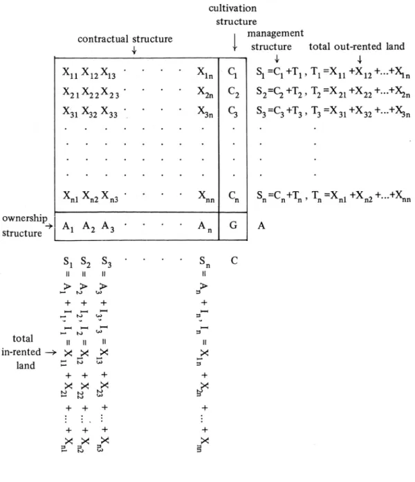
For an agrarian society with n families, the agrarian land structure is presented by a square table with n+1 sectors (i.e., number of columns or rows, see Table 1). The table has three component parts: the cultivation structure, the contractual structure, and the ownership structure.
(1) The cultivation structure C = Col (C1 C2 …Cn) where Ci is the units of land cultivated by the i-th family.
(2) The contractual structure X = Xij (i = 1, 2, … n; j = 1, 2, …n) where Xij is the unit of land rented by the j-th family from the i-th family, i.e., the i-th family is the “creditor” and the j-th family is the “debtor”. (Notes that all the diagonal entries X11 = X22 = … = Xnn = 0 by definition).
We may define,
(1.1a) Ti ≡ Xi1 + Xi2 + … + Xin (i = 1, 2, … n) …….out-rented land (1.1b) Ij≡ X1j + X2j + … + Xnj (j = 1, 2, … n) ……. in-rented land
Where Ti is the total out-rented land (Ij is the total in-rented land) by the i-th family (the j-th family). The sum of all elements in every one of the first n rows is then
(1.2) Si = Ci + Ti (i = 1, 2, … n)
Where Si is the total land managed by the i-th family as it is the sum of his out-rented land and the land he himself cultivates. The land management structure S = (S1, S2, … Sn) is written at the right hand margin of the Table 1. (Notice that the sum of all elements in any row adds up to Si).
Notice that the land the i-th family manage must be at least as his in-rented land, i.e.,
(1.3) Ii≤ Si (i = 1, 2, … n)
because the in-rented land (Ii) must either be cultivated by the family itself or rented out to other family.
4
Table 1: Agrarian Land Structure
(3) The land ownership structure A = (A1, A2, … An). In addition to the cultivation structure (C) and the contractual structure (X), the third part of the agrarian land structure is the land ownership structure (A). When C and X are given, let us define for each family
(1.4) Ai = Si – Ii (i = 1, 2, … n)
Notice that equations (1.2) and (1.4) imply
5
which shows that Ai is the land owned by the i-th family. In other words, the sum of in-rented land (Ii) and land owned (Ai) equals to the sum of out-rented land (Ti) and cultivated land (Ci). The row vector A = (A1 A2 … An) defined in equation (1.4) is the land ownership structure written in the last row of Table 1. (Notice that equation (1.5) implies that the agrarian land structure is a “balanced margin table” in the sense that the sum of all elements in any one row equals to the sum of all elements in the like numbered column).
The existence of the land contractual structure (Xij) signified a separation of the land ownership from the land cultivator-ship. To see this, let the sum of all elements in the last row and column be denoted by
(1.6a) C = C1 + C2 + … Cn ……total land cultivated
(1.6b) A = A1 + A2 + … An ……total land owned
Equation (1.4) immediately implies,3
(1.7) C = A
Which shows the coincidence of the total landed wealth from the social viewpoint (C) and the individual family viewpoint (A). The contractual structure exists merely to separate the ownership and the cultivator-ship to enhance the efficiency of land utilization.
A crude stratification of families into a land-owning class and a landless class is identifiable from the ownership structure (A). Notice that equation (1.3) implies that Ai as defined in equation (1.4) is non-negative.4 Thus the family is a land-owning (landless) family if and only if Ai > 0 (Ai = 0).
SECTION II: THEORETICAL CLASSFICATION OF AGRARIAN FAMILIES
From the abstract model defined above, we can logically deduced exactly nine types of agrarian families as shown in the cells of Table 2.5 These family types indicated by I, II, … IX are shown in the nine cells where a descriptive name is attached to each of them.
3
This follows from the elementary fact that a square table is a balanced margin table when and only when n – 1 sector is in balance.
4
Hence, the agrarian land structure is always a non-negative balanced margin table which is the mathematical foundation of analysis in the next section.
5
Since every number in the quadruplet (Ai, Ci, Ii, Ti) can be either positive or zero, there are altogether
24 = 16 cases as shown in the 16 cells of Table 2. However, it can be readily shown that only nine of these cells are mathematically possible and hence the impossible cases are crossed out.
6
Table 2: Classification of Agrarian Families
The families are classified by a “double standard”. On the one hand, they may be classified according to land ownership (Ai) into “landed” (Ai > 0) and “landless” (Ai = 0) as shown on the left-hand margin. On the other hand, they may be classified by land cultivator-ship (Ci) into “Cultivating” (Ci > 0) and “non-cultivating” (Ci = 0) indicated on the top margin. This double dichotomy is readily recognized to be the most basic classification of agrarian families.
The families may again be classified by two additional standards. On the one hand, they may or may not in-rent land (Ii > 0 or Ii = 0) as shown in rows (1) to (4). On the other hand, they may or may not out-rent land (Ti > 0 or Ti = 0) as shown in columns (1) to (4).
Notice that when a landless family (Ai = 0) does not in-rent any land, it implies that this family is indeed not observable.6 Hence the cells in the last row of Table 2 are crossed out. Similarly, we cannot observe a non-cultivating family that does out-rent any land, and hence the last column of Table 2 is crossed out. Thus Table 2 indicates that there are precisely nine types of agrarian families which are theoretically possible.
6
For Ai = Ii = 0 implies Si = Ci + Ti = 0 by equation (1.5). Hence, the column and row of the i-th sector
7
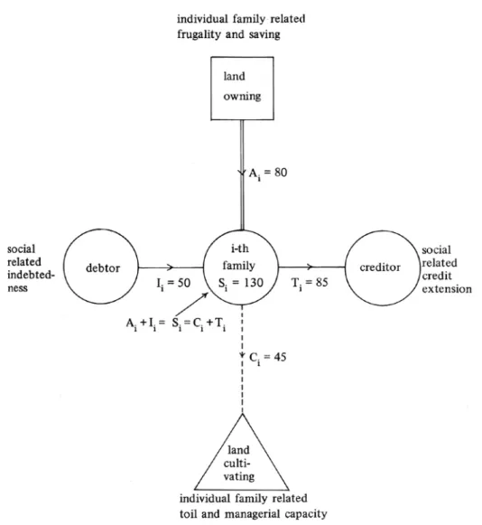
Diagram 1: Four dimensions of a Family’s Status
There are four dimensions that determine the status of an agrarian family, namely, ownership (Ai), cultivator-ship (Ci), creditor-ship (Ti) and debtor-ship (Ii). This is shown in Diagram 1 where the i-th family is represented by a circle in the middle and where the four qualifications are indicated by the arrows linking them with the i-th family. Equation (1.5) is shown by the fact that total inflows into the i-th family (i.e., Si = Ai + Ii = 130) must always be equal to the total out-flows (i.e., Si = Ci + Ti = 130). The nine family types of Table 2 are derived by the identification of all possible cases where some of the values of the quadruplet (Ai, Ii, Ci, Ti) are zero. A diagrammatic representation of each type of family according to this scheme is shown in each cell of Table 2. Notice that in each case, the dimension with the value of zero is not a character of the type and thus is omitted.
This morphological devise suggests that the socio-economic status of an agrarian family is identifiable by an individual family related dimension as well as a
8
social dimension. The former is given by arrows (Ai, Ci) pointing downward while the latter is represented by arrows (Ii, Ti) pointing horizontally to the right. The individual family related dimension specifies that what contribute to determine a family’s status are certain meritorious activities performed by the family. These include antecedent frugality (i.e., saving by the family and its ancestors) leading to land ownership (Ai) and current cultivator-ship (Ci) representing toil and managerial capacity traced to productive technical knowledge and marketing.
The social dimension refers to the given family’s contractual relation with other families in which it may be either a creditor (out-renting land) or a debtor (in-renting land). The so-called landlord-tenant relation, a manifestation of this creditor-debtor relation, is usually associated with a contemporary radical value judgment that attached a higher social status to the creditor (landlord) that “exploits” the debtor (tenant). While this exploitation view is debatable from a historical perspective,7 the fact that a creditor is honored with a higher status is traced basically to the economic reality that it extents credit to the debtor, a division of labor between savers and users of a most important capital asset in an agrarian economy, namely, land. In view of the individual family and social dimensions, a class oriented interpretation of the nine types seems to have a rational economic foundation which is far more complex than it is ordinarily supposed.
There are three types of families indicated by a star (*) in Table 2. These are statistically non-observable types. The very non-observable nature of these types will be explained by a functional approach below. To simplify our analysis at this stage, let us first concentrate on the nomenclature of the six observable types.
2.1 Observable Types
To start with the most familiar, there are the non-cultivating landlord (type IV, Ai > 0, Ti > 0, Ii = 0) and the landless tenant (type I, Ai = 0, Ci > 0, Ii = 0) that lies at the top and the bottom of the social “totem post”. Next comes the “isolated” owner-cultivator (type II, Ai > 0, Ci >0, Ti = 0, Ii = 0) which cultivates his own land and does not incur any “contractual relation” with other families, i.e., he is contractually isolated.
7
For discussion on the status of landlord and tenant, see for example, Chen Han-seng, pp. 42-53; Dwight H. Perkins, Agricultural Development in China, 1368-1968 (Chicago, 1969), pp. 85-110; Ramon H. Myers, The Chinese Peasant Economy; Agricultural Development in Hopei and Shantung,
1890-1940 (Cambridge, Mass., 1970), pp. 217-240; Jing Su and Luo Lun, trans. by Endymion
Wilkinson, Landlord and Labor in Late Imperial China, Case Studies from Shandong (Cambridge, Mass., 1973), pp. 215-218; Liang Keng-yao, ”The land distribution and Tenant system of the Southern Sung,” (in Chinese), Shih-huo Monthly, Vol. 7, No. 10 (January 1978), pp. 500-524.
9
The other three types not only own and cultivate land but also incur at least
some contractual relation, i.e., at least in-rent or out-rent land. When they only in-rent
land, they are called landed tenant (type III, Ai > 0, Ii >0, Ci > 0). Conversely, when they only out-rent land, they are called cultivating landlord (type V, Ai > 0, Ci > 0, Ti >0). Finally, the most complicated one is type VI which not only rents out but also rents in land (Ai >0, Ci >0, Ti >0 Ii >0). At this stage of our analysis, the outstanding peculiarity is that this type of family acts almost like a financial agent or broker that may be called a re-renting class (type VI). It should be noted that it is the only re-renting class which is observable from our empirical data. This implies that a re-renting class is necessary both a landlord and a tenant.
2.2 Non-observable Types
There are three types of families that are not observable from our empirical data. These types are VII, VIII, and IX in Table 2. It should be emphasized that the non-observable nature of these types are characteristic of all localities which have been investigated for this study. The question that naturally arrives is why it is so? Notice from Table 2, there are altogether four types of families that exhibit a re-renting capacity. The three non-observable types all belong to this re-renting category. In other words, the only observable type in the re-renting category is type VI which differs from the three non-observable types in that it both owns and cultivates land. This suggests that a family does not have a re-renting capacity if it does not own land (e.g., type VIII) or does not cultivate (e.g., type VII), or does not do both (type IX). Thus our statistical evidences demonstrate conclusively that land ownership and cultivator-ship are prerequisites for a re-renting capacity.
Unlike a modern urban economy, the farming families do possess technological knowledge of production. Indeed, the very definition of family farm implies a coincidence of a family and a production unit basically different from an urban family. Moreover, traditional agricultural production is characterized by absence of efficiency of large scale production and hence joint ownership is not needed.8 Finally, when a natural disaster (flood, drought, etc.) occurs, it hurts the entire village at the same time and the risk sharing principle is not applicable. So that in a traditional community based on agricultural production, there is no need for specialized credit institutions to
8
Among the villages investigated for this study, we have found that in Pai-ch’i 白企, Chien-ts’un 簡村, and Nan-sha 南沙, there are altogether 36 plots of land each owned by more than one owner. This phenomenon should not be confused with the concept of joint ownership discussed here. For this phenomenon of multiple right, see John Fincher, “Land Tenure in China: Preliminary Evidence from a 1930’s Kwangtung Hillside,” Ch’ing-shih wen-t’i, Vol. 3, No. 10 (November, 1978), pp. 69-81.
10
separate the management and ownership of real capital assets. This is why the three types (VII, VIII, and IX) are not observable.
SECTION III: AGGREGATED AGRARIAN LAND STRUCTURE
The agrarian land structure in Table 1 is defined generally for n families. Since there are theoretically nine types of families, we can group the families into nine sub-classes so that families of each type appear adjacently corresponding to the nine types.9 When Table 1 is consolidated, the result is a 10x10 table as shown in Table 3. In this aggregated agrarian land structure the family types are represented by the first nine sectors. As in Table 1, this aggregated land structure is a balanced margin table in which the last sector is indicated by the capital letter G.
Table 3: A Numerical Example of Agrarian Land Structure
A holistic perspective of the inter-group relation shown in Table 3 is represented by the liner graph in Diagram 2. In this diagram, the cultivator-ship (Ci) is written on the dotted edge while the ownership (Ai) is indicated on the double edge. A solid edge
9
In other words, the first n integers are partitioned as follows:
(1, 2, … n) = ((r11, r12, …, r1n1) (r21, r22, …, r2n2) … (r91, r92,…, r9n9)),
Where n1 + n2 +… +n9 = n and each segment contains all families of a [articular family type forming a group. Table 3 conceptually is a consolidation of the original (n + 1) x (n +1) table shown in Table 1. Notice that the consolidation of a balanced margin table leads to a balanced margin table.
11
represents the creditor-debtor relation. Total inflows always equal total our-flows in every vertex,10 reflecting equation (1.5) in the aggregated sense.
Diagram 2
In the statistical analysis of this paper, we shall accept this aggregated view of Table 3. This means that we shall neglect all intra-group variations and concentrate on inter-group relations and comparisons. The underlying assumption is that the characteristics of all families belonging to the same sub-class are alike. With this class oriented framework, the following sections will take turns to analyze the component parts of the agrarian land structure theoretically and then empirically.
SECTION IV: LAND OWNERSHIP STRUCTURE
For an agrarian community consisting r classes with total land acreage of A units, its class land owning pattern may be written as:
(4.1a) →
A = (A1, A2, … Ar) …… class land owning pattern
10
Notice that Diagram 1 corresponds to Diagram 2 as follows: a doted (solid) edge corresponds to a dotted (solid) edge, etc. For the liner graph of Diagram 2, there are cyclematic number μ = E – V + 1 = 17 where E is the number of edges and V is the number of vertices. Hence we know that in this community, there are 17 identifiable chains of claims.
12
A = A1 + A2 +… + Ar, where Ai is the land acreage owned by families in the i-th class.
The class membership pattern of this community can be written as:
(4.1b) →
N = (N1, N2, … Nr) ……class membership pattern
N = N1 + N2 + … + Nr, where Ni is the number of families consisted in the i-th class. With A and N given for such as community, the endowment ratio can be computed as:
(4.1c) A* = A/N ……endowment ratio
Moreover, the class ownership fraction and the class membership fraction can be computed as:
(4.2a) →
g = (g1, g2, …, gr) = A1/A, A2/A, … Ar/A), and g1 + g2 + … +gr = 1
where gi is the land owning fraction of the i-th class.
(4.2b) →
h = (h1, h2, …, hr) = (N1/N, N2/N,…, Nr/N), and h1 + h2 + … + hr = 1
where hi is the membership fraction of the i-th class.
Since land is the major capital asset of an agrarian community, the land owned by a family reveals its wealthiness, thus the class affluence may be measured by:
(4.3) →
U = (U1, U2, …, Ur) = (A1/N1, A2/N2,…, Ar/Nr) ……class affluence structure
By the concept of aggregated agrarian land structure, we assume that each family of the i-th class owns the same amount of land, and thus Ui indicates the characteristic amount of land owned by the i-th class.
Furthermore, let
(4.4) U1 < U2 < … < Ur
be in a non-decreasing order showing that the class affluence is ranked from poorest to the richest such that 1, 2, …, r shows the class affluence ranks from the poorest to the richest.
Since we have
(4.5a) U1h1+ U2h2+…+ Urhr = (A1/N1)(N1/N)+(A2/N2)(N2/N) + … + (Ar/Nr)(Mr/N) = A/N = A* …… by (4.2b) and (4.3)
13
which shows that the endowment ratio (A*) is the weighted average of the class
affluence structure (
U
→) with the class membership fraction (hi) as the weight. Equation (4.5a) can be written as:
(4.5b) (U1, U2, …, Ur)
�
h1 ... hr�
= A*We may choose the unit of measurement of land such that A* = 1. Thus when
U
→ is divided by A*, we can compute the degree of class land owning as:
(4.6) →
J = (J1, J2, …, Jr) = (U1/A*, U2/A*,… Ur/A*),
where Ji is the degree of land owning of the i-th class.
We may divide
J
→ into three sections: Ji > 1, Ji = 1, Ji < 1. The cases of Ji = 1 may or may not exist, however, the cases of Ji > 1 and Ji < 1 will certainly exist. The cases in which Ji < 1 means that the land owning degree of the i-th class is less than the endowment ration and hence it belongs to the low class. On the Contrary, in the cases of Ji > 1, the i-th class belongs to the high class.
SECTION V: LAND CULTIVATION STRUCTURE
For the same agrarian community of r classes, its class land cultivating pattern may be written as:
(5.1a) →
C = (C1, C2, …, Cr) ……class land cultivating pattern
Where C = C1 + C2 + … + Cr = A …… by (1.7), and (5.1b) C* = C/N = A/N = A* …… by (4.1c)
Moreover, the class land cultivating fraction can be computed as: (5.2) →
t = (t1, t2, …, tr) = C1/A, C2/A,…, Cr/A), and t1 + t2 + … + tr = 1
where ti is the cultivating fraction of the i-th class. And the class land management structure can be shown as:
14 (5.3) →
V = (V1, V2, …, Vr) = (C1/N1, C2/N2, …, Cr/Nr)
where Vi is the characteristic amount of land managed by the i-th class. Since we have
(5.4a) V1h1 + V2h2+…+Vrhr = (C1/N1)(N1/N) +(C2/N2)(N2/N)+ … + (Cr/Nr)(Nr/N) = C/N = A* …… by (4.2b), (5.1b) and (5.3)
This shows that the endowment ration is also the weighted average of the class land management structure with the class membership fraction as the weight. Equation (5.4a) can be rewritten as:
(5.4b) (V1, V2, …, Vr)
�
h1... hr�
= A*
→
When V is divided by A*, the degree of class land management can be computed as:
(5.5) →
K = (K1, K2, …, Kr) = (V1/A*, V2/A*, …, Vr/A*)
Where Ki is the degree of land management of the i-th class. We can also divide
𝐾
→ into three sections: Ki < 1, Ki = 1, Ki >1. In the cases in which Ki < 1, the land cultivated by the i-th class is less than its own supply of labor force (i.e., supposed the class membership fraction represents the labor force) can manage and the i-th class has lost interest in agricultural management. On the contrary, in the cases in which Ki�nk� > 1, the land cultivated by the i-th class is more than its own supply of labor force can manage and the i-th class has increased interest in agricultural management and may have to hire laborers from the labor market.
SECTION VI: CLASS RANKING ORDER
When we arrange the classes according to the class affluence rank (Ui) as shown in the formula of (4.4), we are not able to arrange them simultaneously according to the class land management (Vi). Thus we should choose only one for the class making order and in this paper the class affluence ranking order is our choice. When the class membership fraction (hi) is measured on the horizontal axis and the class land owning fraction (gi) on the vertical axis, both according to the class
15
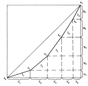
affluence ranking order, we will obtain a Lorenz curve of class land ownership as shown in Diagram 3 with a five-class community as an example. Equation (4.4) implies that this curve is convex. The slope of (ai-1 ai) can be computed as:
(6.1) slop of (ai-1 ai) =gi/hi = (Ai/A)(Ni/N) = Ui/A* = Ji ……by (4.2b) and (4.6)
Thus, the slope of (ai-1 ai) indicates the degree of class land ownership. Depended on whether Ji > 1 or Ji < 1, the division of high and low classes can be immediately discerned from this curve.
Diagram 3: Lorenz Curve of Class Land Ownership
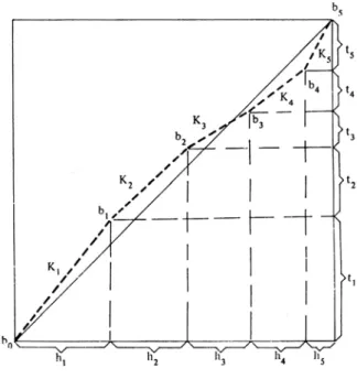
When the class membership fractions are measured as before, while on the vertical axis the class land cultivating fraction (ti) are measured correspondingly according to the class affluence ranking order, we will obtain a pseudo Lorenz curve
of class land cultivator-ship as shown in Diagram 4. The pseudo Lorenz curve of class
cultivator-ship is not necessarily convex as the orders of class affluence rank and the class land management rank are not coincidence. The slope of (bi-1 bi) can be computed as:
(6.2) slope of (bi-1 bi) = ti/hi = (Ci/A)(Ni/N) = Vi/A* = Ki ……by (4.2b), (5.3) & (5.5)
Thus, the slope of (bi-1 bi) indicates the degree of class land management.
16
Diagram 4: Pseudo Lorenz Curve of Class Land Cultivatorship
With the Lorenz curve of class land ownership and the pseudo Lorenz curve of class land cultivator-ship derived from the methods discussed above, we may furthermore measure the degree of inequality of land ownership distribution by the former and the degree of concentration of land management by the latter. These will be discussed in turns below.
SECTION VII: INEQUALITY OF LAND OWNERSHIP DISTRIBUTION
Referring to Diagram 3, we may compute the Gini coefficient to indicate the degree of inequality of land ownership distribution. If the area under Lorenz curve is denoted by A, then a traditional method of computing the Gini coefficient is:
(7.1) G = 1-2A
Moreover, the Gini coefficient can also be computed as the average fraction gap when individual family data is used.11 We may apply this method here by using group data. Since Ji is the degree of class land ownership and it is monotonically non-decreasing on the Lorenz curve, the difference of (Ji - Jj) where i ≥ j shows the gap of the degree of land ownership between a higher class and a lower class. When
11
See John C. Fei, G. Ranis, and S. Kuo, Growth with Equity: The Taiwan Case (New York and London, 1979), pp. 331-333.
17
the group data are used, the group fraction should be taken as the weight. Since we have
(7.2) (J1, J2, …, Jr) = � hi
⋮
hr� = 1 …… by (4.5b) and (4.6)
we may compute the sum of all gaps of the degree of land owning as follows, using a five-class example: h1 h2 h3 h4 h5 h1 0 J2-J1 J3-J1 J4-J1 J5-J1 h2 0 J3-J2 J4-J2 J5-J2 h3 0 J4-J3 J5-J3 = h2h1(J2-J1) + h3h1(J3-J1) +…+h5h4(J5-J4) h4 0 J5-J4 h5 0
A term such as h2h1(J2-J1) indicates the weighted fraction gap of the degree of land owning between class 2 and class 1, and the former is ranked higher than the latter. Thus, the Gini coefficient is exactly the sum of all weighted fractional gaps of the degree of land owning, it can be written as:12
r
(7.3) G = ∑ hihj (Ji – Jj), where i ≥ j j=1
SECTION VIII: CONCENTRATION OF LAND MANAGEMENT
As shown in Diagram 4, the distribution of class land cultivator-ship based on the class affluence rank is represented by a pseudo Lorenz curve. To measure the degree of concentration of land management by such a curve, we may first tackle this problem by a diagrammatic explanation. In Diagram 5 the pseudo Lorenz curve of class land cultivator-ship are shown in five different positions denoted by A to E. The degree of concentration of land management depicted by these five curves may be expressed literarily as follows:
12
18 Diagram 5
A: extreme low class concentration B: moderate low class concentration
C: equal concentration
D: moderate high class concentration E: extreme high class concentration
Let the Gini coefficient measuring the degree of concentration of land management based on the pseudo Lorenz curve be denoted by G*, then in the above five position, the values of G* are as follows:
A: G* = -1 B: -1 < G* < 0 C: G* = 0 D: 0 < G* < 1 E: G* = 1
Referring back t Diagram 4, since Ki indicates the degree of class land management, we can calculate G* by the same method of G as shown in section VII. G* is the sum of all weighted fractional gaps of the degree of class management and can be written as:
r
(8.1) G* = ∑ hihj (Ki – Kj), where i ≥ j j=1
Since Ki may not exist in a monotonically non-decreasing order, some terms of hihj (Ki – Kj) may be negative and hence G* may be negative in some cases.
19
SECTION IX: CONTRACTUAL STRUCTURE
9.1 A Simplified Two-class Model
In an agrarian society, the institution of land tenancy is used to enhance the efficiency of land utilization when the land ownership and cultivator-ship are not coincided with the same family. This land contractual problem may be first understood by a simplified two-class model. Diagram 6 shows the Lorenz curve of class land ownership with a class breaking point at A. When A is fixed, two marginal cases of class land cultivation are indicated by M- and M+ respectively. The meanings of these two marginal cases are as follows:
(1) At point M-, the fractions of land cultivated by the two classes are exactly the same as the fraction of land owned by them respectively.
(2) At point M+, the fractions of land cultivated by the two classes exactly corresponding to the class membership fraction (or the supply of labor force) of the two classes.
In Diagram 6 the vertically shaded area indicates the existence of land tenancy. At the area above M-, the high class rents out its land to the low class, while at the area below M-, the phenomenon of negative tenancy occurs when the low class rents out its land. Thus a conclusion at this point is that when the land owning distribution is given in an agrarian society, the more the high class loses interest in land cultivation (management), the more the land tenancy will prevail.
20
The phenomenon of land tenancy can be further analyzed with the comparison between the Lorenz curve of class land ownership and the pseudo Lorenz curve of class land cultivator-ship. Diagram 7 depicts a sequence of pseudo Lorenz curve (dotted) in contrast to a fixed Lorenz curve (solid) of the two-class model.
Diagram 7
Thus we can see when the class land ownership distribution is given in an agrarian society (i.e., the Lorenz curve is fixed), the prevalence of land tenancy will shift with the relative distribution of cultivator-ship (i.e., the relative position of pseudo Lorenz curve). A few remarks may be made here.
(1) When the pseudo Lorenz curve shifts upwards, the low class gradually increases interest in land cultivation. The process of shifting may go through three steps:
(a) At the area below M-, the high class has the greatest interest in land cultivation, the pseudo Lorenz curve lies bellows the Lorenz curve.
(b) At the area between M- and M+, the high class gradually loses interest in cultivation; the pseudo Lorenz curve shifts upwards above the Lorenz curve. (c) At the area above M+, the high class drain its interest in cultivation; the pseudo
Lorenz curve shifts further upwards above the 45 degree line.
(2) With the distribution of class land ownership given, the result of losing interest in cultivation from the part of high class is the increase in land tenancy. This can be seen from the gap between the Lorenz curve and the pseudo Lorenz curve. Since with any pair of the Lorenz curve and the pseudo Lorenz curve we may
21
compute G and G* (see equation (7.3) and (8.1)), thus comparing the curve in Diagram 7, we can see the prevalence of land tenancy in different circumstances as follows:
marginal case
0 < G < G* = 1 extreme negative Below M- 0 < G < G* <1 negative tenancy
0 < G = G* < 1 no tenancy Between M- and M+ 0 < G* < G <1 positive tenancy 0 = G*<G < 1 perfect tenancy accommodation Above M+ -1 < G* < 0 < G < 1 increasing positive -1= G* < 0 < G <1 extreme positive
Let the gap between the Lorenz curve and the pseudo Lorenz curve be measured as portion of the area between the Lorenz curve and the 45 degree line, such as:
(9.1) x = (G – G*)/G
where x may be called the concentration index indicating the degree of land management concentration to the low class.
(3)To investigate into the causes of prevalence of land tenancy, we must focus on two aspects: (a) the equality in distribution of land ownership and (b) the maintenance of land cultivating interest by different social classes.
9.2 Degree of Land Tenancy
In addition to concentration index (x), the degree of land tenancy may also be measured be the gap between the class affluence and the class land management. Since we have
(9.2a) U1h1 + U2h2 + … + Urhr = V1h1 + V2h2 + … + Vrhr …… by (4.5) and (5.4) thus,
(9.2b) (U1−V1)h1 + (U2−V2)h2 + … + (Ur−Vr) hr = 0 Or it can be written as:
(9.3c) d1h1 + d2h2 + … +drhr = 0
22
When di > 1, the i-th class is an out-renting class and di is the out-renting amount of land by the i-th class per family;
di < 1, the i-th class is an in-renting class and di is the in-renting amount of land by the i-th class per family;
di = 0, the i-th class is a land self-sufficient class, i.e., the families of the i-th class are isolated cultivators.
From equation (9.2c), we may compute the total amount of rented land as” (9.2d) R = (h1│d1 + h2│d2 + … + hr│dr) / 2
where R is the total amount of rented land per family in the community. Thus the
degree of land tenancy (R*) may be measured as a portion of rented land to
endowment ratio, such as: (9.3) R* = R/A*
In other sense, R* may also be calculated as:
(9.4) R* = (h1│J1−K1│ + h2│J2−K2│+ … + hr│Jr−Kr│) / 2 …by (4.6) and (5.5) This shows that the degree of land tenancy is one half of the weighted absolute gap between the degree of class land owning and the degree of class land management, using the class membership fraction as the weight.
9.3 Correlation between R* and x
With the concentration index (x) computed by (9.1) and the degree of land tenancy computed by (9.3) or (9.4), we may predict that these two indicators of land tenancy are positively correlated for we can see that within the three areas, the values of x are as follows:
(1) below M-: x < 0, where negative tenancy prevail;
(2) between M- and M+: 1 > x > 0, where positive tenancy prevails;
(3) above M+: x > 1, where tenancy increases and the land management concentrated to low class.
In other words, where value of x is high, value of R* is also high. This should be tested with the empirical data.
SECTION X: EMPIRICAL ANALYSIS
The data for empirical analysis are organized from the land records of 17 villages and 3 towns in Kwangtung province during the 1930s (see Appendix). From these land records, we are able to identify six types of agrarian families as has been discussed above in Section II. However, for the sake of simplicity and convenience, the family classification will be modified here. Since there are only a small number of
23
re-renting class (type VI) and the affluence of families belonging to this class varies; one may either be a creditor (net out-rented) or a debtor (ne in-rented), the families of type VI will be reclassified. If a family is a creditor, it will be consolidated into cultivating landlord (type V); if a family is a debtor, it will be consolidated into landed tenant (type III). (See Appendix Table 2a).
With this modification, the relevant statistical data are listed in tables in the Appendix, while in the following discussions some diagrams will be used for illustration.
10.1 Aggregated Agrarian Land Structure
Based on the concept stated in Section III, an aggregated agrarian land structure of six observable types of families at Pai-ch’i 白企 village in Chung-shan 中山 county is presented in Table 4 for an example.
24
The statistical data needed for the aggregated agrarian land structure are listed in Table A1 in the Appendix. The data are listed correspondingly to the three component parts of agrarian land structure and all entries of a locality may be arranged into a balanced margin table as illustrated in Table 4. It is notable that among 20 localities investigated for this study, only two (Shang-hsia-wo 上下窩 village and Ma-an 馬安 town) have no families belonging to the re-renting class (type VI). Since the families belonging to this type have been reclassified (see Table A2), in the analysis below, all localities will have five types of families constituting five sub-classes.
10.2 Class Affluence Ranking Order
Although we have denoted the five sub-classes in the order of 1 to 5 ranking from the landless tenant to the cultivating landlord, the empirical data of the 20 localities demonstrate that this ranking order is not always held (see Table A6). There are only 9 localities, Pai-ch’i 白企, Ta-ch’e 大車, San-chou 珊洲, T’ang-t’ou 塘頭, Hsien-men 仙門, Ch’ih-chaio 赤窖. P’ing-kung 坪宮, Ma-lan 馬欄, and P’ing-hai 平 海, have the class affluence ranking order conforms to the family type notation (i.e., U1 < U2 <U3 < U4 < U5), while the other 11 localities have shown variations. However, the variations in most cases are only a change of order between the two adjacent sub-classes. The first kind of variation is U1 < U3 < U2 < U4 < U5; there are 5 localities, Chien-ts’un 簡村, San-tai-mei 三岱美, Hsien-shih 仙市, Nei-ch’i 內七 and Ch’ing-p’ing 慶平, showing this order. The second kind of variation is U1 < U2 < U3 < U5 < U4; there are 2 localities, Nan-sha 南沙 and Ho-heng 和橫, showing this order. The remaining 4 localities reveal rather irregular ranking order such as:
U1 < U4 < U2 < U3 < U5 (2 cases, Hsieh-ts’un 謝村 and Ma-an 馬安) U1 < U3 < U4 < U2 < U5 (1 case, Li-lin 荔林)
U1 < U4 < U2 = U5 < U3 (1 case, Shang-hsia-wo 上下窩).
We consider that these variations are quite natural for the localities investigated are chosen randomly.
Since we have decided to use the class affluence ranking order as the unique reference for class ranking, the Lorenz curve of class land owning and the pseudo Lorenz curve of class land cultivator-ship are derived for each locality according to its ranking order of Ui revealed respectively by the empirical data.
10.3 Division of High and Low Classes
Based on the statistical data listed in Table A4 to A7, Lorenz curve (solid) of class land ownership and pseudo Lorenz curve (dotted) of class land cultivator-ship
25
/derived by the methods discussed in sections VII and VIII can be drawn for each locality. As mentioned above, the ranking order of Ui varies among these localities, thus, here we have chosen one locality in each case to illustrate different patterns of ranking order. Diagram 8.1 demonstrating the monotonically non-decreasing order of J1 < J2 < J3 < J4 < J5; Diagram 8.2, the order of J1 < J3 < J2 < J4 < J5; Diagram 8.3, the order of J1 < J2 < J3 < J5 < J4; Diagram 8.4 the order of J1 < J4 < J2 < J3 < J5; Diagram 8.5, the order of J1 < J3 < J4 < J2 < J5 and Diagram 8.6, the order of J1 < J4 < J2 = J5< J3.
26
27
28
29
30
Diagram 8.6: Shang-hsia-wo
If Ji ≥ 1 be taken as an indicator for dividing these sub-classes into two major classes – high class and low class – then we can see the breaking point (A) also varies among these 20 localities. Most frequently (18 cases among 20 with exceptions of Ma-an and Shang-hsia-wo), sub-classes 4 and 5 fall within the area of high class, while the status of sub-classes 2 and 3 are rather instable as they may be high or low. It is notable that in the two exceptional cases, Ma-an and Shang-hsia-wo, the sub-class 4 falls within the area of low class. However, only the case of Shang-hsia-wo (see Diagram 8.6) shows negative tenancy while the case of Ma-an does not. This is because only in the former case the condition of 0 < G < G* < 1 is fulfilled. It is also notable that in these two localities, the land owning fraction of
31
sub-class 4 (g4) is rather small (0.022 in Ma-an and 0.054 in Shang-hsia-wo). Thus, a next question to be asked is which sub-class is predominant in an agrarian community? Obviously, this question should not be dealt with merely from the point of class membership (i.e., the group size), it should at least be analyzed by taking class land ownership and/or cultivator-ship into consideration at the same time.
10.4 Class Predominant Pattern
Turning to this question, let us first look at the shape of Lorenz curve with Gini coefficient (G) measuring the degree of inequality in land ownership distribution. Among the 20 localities, we see that the values of G range between 0.123 and 0.533 (see Table A8, locality Nos. 20 and 10). The former case shows that sub-class 2 owns the lion share of land and may be called as the isolated cultivator predominant pattern (ICP pattern); this pattern implies that the share of sub-class 4 is comparatively small. There are 4 other cases (Ho-heng, Hsieh-ts’un, Ma-an and Li-lin) demonstrating the ICP pattern (see Table A4, Col. h2; Table A5, Col. g2).
In contrast to the ICP pattern, we can see in most of the other localities sub-class 4 owns the largest share of land and this may be called the non-cultivating landlord predominant pattern. Since this pattern also implies that the landless tenant is predominant from the respect of land cultivation, and hence it may also be called as the landless tenant predominant pattern (LTP pattern). Among the 15 cases demonstrating the LTP pattern, we can also discern variations which reflect a secondary predominance of another sub-class besides the predominant one. For example, the cases of Ta-ch’e, T’ang-t’ou, P’ing-kung and Ma-lan show that sub-class 3 is also predominant in land cultivating (see Table A5, Col. t3), while the case of Chien-ts’un and Nei-ch’i show that sub-class 5 is also predominant in land owning (see Table A5, Col. g5), although in terms of membership, the secondary predominant sub-class is comparatively smaller (see Table A4, Cols. h3, h5).
Furthermore, we may look at the shape of pseudo Lorenz curve with pseudo Gini coefficient (G*) meaning the degree of land management. It is quite reasonable to find that the values of G* are positive (0 < G* < 1) in the five cases demonstrating the ICP pattern (see Table A8). As shown in a simplified two-class model, the condition 0 < G* < 1 indicates moderate high class concentration (see Section VIII). Among these five cases, three have the predominant sub-class 2 falling in the area of high class, while the other two cases do not. This result reveals that the status of sub-class 2 is uniform in all places.
Among the 15 cases showing the LTP pattern, the values of G* range between -0.541 and -0.089 (see Table A8, locality Nos. 5 and 4). In terms of two-class model,
32
the condition -1 < G* < 0 indicates moderate low class concentration. Within the observed range of G*, we can see that the LTP pattern is more outstanding in the cases in which G* values are closer to -0.5 (see Table A8, locality Nos. 3, 5, 6, 9, 11, 12, 14, 15).
From the above analysis and comparison on the empirical data of 20 localities, we are able to conclude that there are two major class predominant patterns related to inequality of land ownership distribution and concentration of land management. On the one hand, the ICP pattern goes with relatively equal land ownership distribution (i.e., smaller G) and moderate high class concentration of management (i.e., Positive G*). On the other hand, the LTP pattern goes with relatively unequal land ownership distribution (i.e., larger G) and moderate low class concentration of management (i.e, negative G*).
10.5 Prevalence of Land Tenancy
The next question to be analyzed is the prevalence of land tenancy and its relation to the two curves. As stated in equation (9.1), the concentration index (x) measures the difference of the Gini and pseudo Gini coefficients (G – G*) as the fraction of the Gini coefficient (G). Diagrammatically, this is to see how large the proportion is that total area between the two curves (vertically shaded area) as to the area between the 45 degree line and the Lorenz curve (horizontally shaded area). The value of x for each locality is listed in Table A8. We may easily divide these 20 localities into three groups as follows:
The ICP pattern:
(1) 0 > x: locality No.20, negative tenancy;
(2) 1 > x > 0: locality Nos. 16-19, moderate tenancy; and the LTP pattern
(3) X > 1: locality Nos. 1-15, high tenancy.
Thus, it is quite clear that where the value of x is higher, the land tenancy is more prevalent.
Moreover, in equation (9.3) and (9.4), the degree of land tenancy (R*) is measured as the proportion of total rented amount of land to the endowment ration and as one half of the weighted absolute gap between the degree of land owning and the degree of land management. Also listed in Table A8 are values of R* for 20 localities.
To see whether these two indicators of land tenancy are correlated, a linear regression by the ordinary least square method produces a result of coefficient of
33
determination as 0.867 (see Diagram 9). Thus, we may say that the empirical implementation in this aspect is quite satisfactory.
Diagram 9
10.6 Interpretation on Empirical Findings
From the above analysis on empirical data of 20 localities, a major finding is that the class oriented agrarian land distribution reflects institutional arrangements adopted by an agrarian community to accommodate its labor force to land utilization under given circumstances. The two predominant patterns immediately reveal whether the arrangement through land tenancy has been adopted or not in a locality. We shall try to provide some interpretations on the empirical findings here.
From most literature dealing with the subject of land tenancy in the early twentieth-century China, we can derive two generations: (1) the prevalence of land tenancy differed pronouncedly in the North and the South, and even within the same province and (2) the land tenancy was high in areas which were more commercialized.13
The empirical findings from 17 villages and 3 towns in 12 counties of Kwangtung province demonstrated conclusively that variations did exist in the same
13
See for example, R. H. Tawney, Land and Labor in China (original, 1932; reprint, Boston, 1966), pp. 63-69. Dwight H. Perkins, pp. 85-110; Joseph W. Esherick, “Number Games: A Note on Land Distribution in Pre-revolutionary China,” Modern China, Vol. 7, No. 4 (October, 1981), pp. 387-411.
34
province. Thus the first generalization mentioned above is proved valid. We should only concentrate on testing the validity of the second generalization through the use of other available data organized from the same land records.
The first available data other than land acreage is land price. If it is reasonable to assume that the unit price of land reflects the fertility of land and that the higher the fertility of land in a place the more commercialized it is, then the unit price of land may be taken as an indicator for commercialization. By using this indicator, we should be aware of the fact that land price may be varied to some extents in different areas. For example, among the localities we have studies for this paper, the unit price of land at five villages in Ch’eng-hai 澄海 county is much higher than that in other counties. Of course, Ch’eng-hai county is nearby a commercial center, Shan-t’ou 汕 頭 (Swatow), and this may be a reason for its high price of land. However, we have also investigated a few villages in P’an-yü 番禺 and Nan-hai 南海 counties which are nearby another commercial center, Canton, and yet the land price at these villages are not particularly high. Due to these variations, the results of correlation analysis may be affected (see Table A9).
For example, if we take the class membership as a proxy for labor force and let the sum of numbers of landless tenant (N1) and one half of landed tenant (N3/2) be a proxy for the tenant labor force (Nt), we have found that there is a rather weak positive relationship between the tenant labor force (Nt) and the unit price of land (p); the coefficient of determination is only 0.155 (see Diagram 10).
35
If we should look into land price for any further interpretation, we may have to try from another angle. For instance, we are able to arrange the data of land price corresponding to class land ownership and calculate the unit price of land owned by each sub-class as shown in Table A9. Despite the variations among localities, we can see that among the sub-classes of a locality, the unit price of land owned by landed tenant (p3) is the lowest in 12 localities and the next lowest in 4 localities. This may be interpreted as that when a landless tenant has accumulated enough savings to purchase land to promote himself into the status of a landed tenant; he is most likely to buy the cheapest land. However, this interpretation will not be applicable to the remaining 4 localities where the unit price of land owned by sub-class 3 is the highest or the next highest.
Another dimension of the data available from the land records is fragmentation of land. If we assume that in a place of higher land tenancy there will be fewer plots of minimum size land and hence it is more difficult for the poor tenant to purchase land, we may find a negative relationship between the prevalence of land tenancy and land fragmentation. When the concentration index 9x) is taken as a dependent variable and the ratio of minimum size plots to the total plots of land (m) is taken as an independent variable, the scatter diagram reveals that there is negative relationship between these two variables. A regression by the ordinary least square method produces a result of coefficient of determination as 0.0583 (see Diagram 11). But it should be noted that this result is obtained when one of the extreme case (m = 0.424) is deleted.
36
Finally, the last dimension of data available from the land records is rent. Except for the case of Chine-ts’un where only plots rented out have rent in records, for all other localities, rent is recorded for every plot of land regardless whether it is rented out or not. For this reason, we tend to suppose that the recorded rent may be the rent paid by the tenant to the owner. Moreover, in four localities (P’ing-kung, Ch’ing-p’ing, Li-lin, and Shang-hsia-wo) the recorded rent is in terms of kind with different unit of accounting and this increases difficulties of analysis.
Since we are not able to find any significant relationship between the unit rant computed from the records and the concentration index (x) using the data of 15 localities, at this stage, we should say that the recorded rent may not be used directly to test whether it is a reflection of commercialization and is related to land tenancy. Using the pertinent data from the same land records, we have tried in above to test the hypothesis on the relationship between commercialization and land tenancy. We have found that at least from the aspect of land price, commercialization and land tenancy were positively related and from the aspect of land fragmentation, they were negatively related, although the degree of correlation were, in both cases, quite weak due to variations in the original data.
We should also consult other documents to elaborate our interpretation. However, most local gazetteers of the counties related to this study do not provide detail information down to the village level. For this reason, these findings from the land records are all the more valuable as they add new historical evidences that are not available elsewhere.
CONCLUDING REMARKS
Starting from an abstract concept of agrarian land structure, we have set up a theoretical framework for empirical analysis n land records of Kwangtung in the 1930s. This theoretical framework may be applied to analyze the agrarian land structure in any society as long as necessary statistical data are available.
Empirical analysis and comparison on data organized from the land records of 20 localities demonstrate that the agrarian land distribution is a rather complex framework.
The empirical implementation to the theory has produced quite satisfactory results. From the shapes of Lorenz curve of class land ownership and pseudo Lorenz curve of class land cultivator-ship, we have been able to discern two predominant patterns, the ICP pattern and the LTP pattern, corresponding to certain values of G and G*. Moreover, there is a positive relationship between the two indicators of land tenancy, R* and x. In addition, the hypothesis on the relation between
37
commercialization and land tenancy has been tested through using pertinent data available from the same land records. Thus the intrinsic consistence of the land records is proved.
Finally, it should be emphasized that this voluminous (a total of 3,333 volumes) land records of Kwangtung province are valuable for understanding the agrarian land structure in the 1930s, a critical era of modern land reform. Materials of 20 localities investigated for this study are accounted for only one percent of the whole collection. However randomly and preliminary, the empirical analysis has produced quite good results. Thus it is indeed necessary and worthwhile to further investigate systematically into this huge collection.
APPENDIX
To construct an agrarian land structure for a rural community, it is required to have primary statistical data that reveals the family identity of owner and cultivator of every tract of land in that community. Fortunately, the Taiwan Branch of the National Central Library in Taipei has a collection of Kwangtung land records which provides the necessary data for this study.14
For our purpose, the original records are first transcribed into numerical code and then computerized. For each plot of land, the original records include seven variables: (1) location, (2) grade of land, (3) acreage of land, (4) price of land, (5) rent of land, (6) owner, and (7) tenant (i.e., cultivator). Before the original data are organized into useful statistical data, it is necessary to identify each owner and cultivator according to the classification shown in Table 2 in the text. Since an owner (cultivator) may own (cultivate) more than one plot of land and some owners may also cultivate their own land or other people’s land, in original records the same owner (cultivator) may appear here and there over a wide range of land plots, thus it is necessary to look through carefully all plots in a village to identify the type that one may belong to. With the owner denoted as variable 6 (v6) and the cultivator as variable 7 (v7) for each plot of land, the rule of identification is as follows:
Type I: v6 ≠ v7 where all v7 only appear as cultivator. Type II: v6 = v7.
Type III: v6 = v7 and v6 ≠ v7 where all v6 in the latter are not the same as v6 in the former.
14
For details of this collection see, A Catalog of Kuang-tung Land Records in the Taiwan Branch of
38
Type IV: v6 ≠ v7 where all v6 only appear as owner. Type V: v6 = v7 and v6 ≠ v7 where all v6 are the same.
Type VI: v6 = v7 and v6 ≠ v7 where at least one v6 is not the same.
With the type identification for each owner and cultivator, the eighth variable, namely, the relationship between owner and cultivator of every plot of land can be obtained. With the eight variables ready for every plot of land, then the statistical data can be organized corresponding to types of families. The statistical data needed for analyses in the text are arranges in ten tables as follows:
Table A1: Land Acreage Corresponding to Types of Families: Elements for Aggregated Agrarian Land Structure
Table A2: Reclassification of Type VI Families
Table A3: Land Owning and Cultivating Acreage of Five Sub-classes Table A4: Class Membership
Table A5: Class Land owning and cultivating Structure Table A7: Degree of Class Land management
Table A8: Some Important Indicators Table A9: Land Price
Table A10: Minimum Size Land
In Tables A1 and A2, localities are arranged by counties just to show their administrative affiliation. The last three localities are towns while others are villages. In Tables A3 and A10, localities are arranged corresponding to variations of class affluence ranking order as discussed in the text.
39
Table A1: Land Acreage Corresponding to Types of Families: Elements for Aggregated Agrarian Land Structure
Unit: mou
County Locality
Land Owning (A)
I II III IV V VI Chung-shan Pai-ch’i 0 235.06 111.69 393.35 242.07 59.30 Ta-ch’e 0 49.85 56.06 724.10 80.00 43.57 Shan-chou 0 24.90 14.55 607.67 43.70 29.80 P’an-yü T’ang-t’ou 0 107.60 94.70 333.15 152.95 90.50 Hsieh-ts’un 0 272.35 46.20 198.45 64.60 5.90 Nan-hai Chien-ts’un 0 581.11 10.50 643.24 642.24 39.14 Ch’eng-hai San-tai-mei 0 27.50 32.97 1353.19 4.80 45.63 Nan-sha 0 74.60 25.80 1409.65 32.10 67.20 Hsien-men 0 19.60 23.60 656.65 37.40 41.10 Ch’ih-chiao 0 8.70 23.85 539.45 51.90 14.10 Hsien-shih 0 11.60 4.20 248.00 6.30 0.30 Hsing-ning P’ing-kung 0 21.71 15.44 54.67 21.92 18.20 Wu-hua Shang-hsia-wo 0 47.65 9.64 3.48 3.40 -- Jao-p’ing Li-lin 0 343.80 40.58 41.04 22.45 2.90 P’u-ning Ho-heng 0 435.88 429.81 217.21 71.49 55.67 Ta-p’u Nei-ch’i 0 11.77 19.46 55.60 51.40 9.24 Nan-hsiung Ch’ing-p’ing 0 35.92 39.15 608.19 26.64 30.73 Ho-p’u Ma-lan 0 97.00 102.30 541.50 112.70 91.00 Hui-yang Ma-an 0 491.90 81.20 17.20 176.60 -- P’ing-hai 0 51.30 19.60 432.50 36.70 9.30 County Locality Land Cultivating (C) I II III IV V VI Chung-shan Pai-ch’i 407.65 235.06 270.29 0 87.97 40.50 Ta-ch’e 433.05 49.85 390.21 0 26.15 54.32 Shan-chou 519.97 24.90 77.50 0 16.10 82.15 P’an-yü T’ang-t’ou 266.10 107.60 204.55 0 97.55 103.10 Hsieh-ts’un 206.25 272.35 70.70 0 18.40 19.80 Nan-hai Chien-ts’un 1086.00 581.11 41.02 0 150.74 57.30 Ch’eng-hai San-tai-mei 1222.67 27.50 131.20 0 0.30 84.02 Nan-sha 1372.15 74.60 92.40 0 23.90 46.30 Hsien-men 618.10 19.60 78.40 0 23.90 38.35 Ch’ih-chiao 491.90 8.70 98.30 0 13.70 25.40 Hsien-shih 186.40 11.60 70.10 0 0.60 1.70 Hsing-ning P’ing-kung 26.23 21.71 50.69 0 15.23 18.9 Wu-hua Shang-hsia-wo 1.50 47.65 12.48 0 2.54 -- Jao-p’ing Li-lin 20.58 343.80 75.21 0 2.85 8.35 P’u-ning Ho-heng 38.98 435.88 643.44 0 37.19 54.57 Ta-p’u Nei-ch’i 35.50 11.77 67.30 0 8.63 24.17 Nan-hsiung Ch’ing-p’ing 495.18 35.92 156.49 0 13.31 39.73 Ho-p’u Ma-lan 367.30 97.00 312.30 0 55.40 112.50 Hui-yang Ma-an 28.40 491.90 105.60 0 142.00 -- P’ing-hai 405.70 51.30 68.70 0 12.00 11.70
40 Table A1 (continued)
Unit: mou
County Locality
Land Renting (Xij) Total
A=C X41 X43 X46 X51 X53 X56 X61 X63 Chung- shan Pai-ch’i 278.20 104.65 10.50 98.45 52.95 2.70 31.00 1.00 1041.47 Ta-ch’e 395.55 291.85 37.60 23.90 27.85 2.10 13.60 14.45 953.58 Shan-chou 476.27 54.65 76.75 19.90 7.70 -- 23.80 0.60 720.62 Pan-yü T’ang-t’ou 197.60 94.95 40.60 44.60 5.70 5.10 23.90 9.20 778.90 Hsieh-ts’un 178.55 16.10 3.80 25.00 6.70 14.50 2.70 1.70 587.50 Nan-hai Chien-ts’un 600.66 22.02 20.48 451.02 8.48 32.00 34.32 -- 1916.17 Ch’eng- hai San-tai-mei 1181.89 95.70 75.60 4.50 -- -- 36.28 2.53 1464.09 Nan-sha 1306.45 62.10 41.10 3.70 4.50 -- 62.00 -- 1609.35 Hsien-men 578.50 47.80 30.35 10.90 1.60 1.00 28.70 5.40 778.35 Ch’ih-chiao 453.20 66.15 20.10 30.70 6.00 1.50 8.00 2.30 638.00 Hsien-shih 180.40 65.90 1.70 5.70 -- -- 0.30 -- 270.40 Hsin-ning P’ing-kung 17.88 30.35 6.44 2.40 2.65 1.65 5.95 2.25 131.91 Wu-hua Shang-hsia-wo 1.34 2.14 -- 0.16 0.70 -- -- -- 64.17 Jao-p’ing Lin-lin 15.34 22.07 3.63 4.74 12.42 2.44 0.50 0.14 450.79 P’u-ning Ho-heng 31.22 176.74 9.25 6.18 26.53 1.59 1.58 10.36 1210.06 Ta-p’u Nei-ch’i 20.88 24.65 10.07 13.11 22.04 7.62 1.51 1.25 147.37 Nan-hsiung Ch’ing-p’ing 476.75 113.39 18.05 9.88 2.95 0.50 8.55 1.00 740.63 Ho-p’u Ma-lan 299.00 187.80 54.70 44.00 10.60 2.70 24.30 11.60 944.50 Hui-ynag Ma-an 6.70 10.50 -- 21.70 12.90 -- -- -- 767.90 P’ing-hai 381.60 41.10 9.80 19.10 4.80 0.80 5.00 3.20 549.40
Table A2: Reclassification of Type VI Families
Locality
Consolidated into Type III Consolidated into Type V
N A C P N A C P Pai-ch’i 6 13.20 16.10 552.00 4 46.10 24.40 2188.00 Ta-ch’e 13 13.62 43.82 441.60 3 29.95 10.50 1499.50 Shan-chou 7 14.40 77.50 456.00 1 15.40 5.00 664.00 T’ang-t’ou 21 63.50 86.00 2125.00 4 27.00 17.10 1012.50 Hsieh-ts’un 3 3.30 19.10 27.00 2 2.60 0.70 240.00 Chien-ts’un 13 25.14 52.70 752.30 1 14.00 4.60 980.00 San-tai-mei 19 24.73 72.32 2998.00 8 20.90 10.10 3245.00 Nan-sha 5 52.80 37.30 856.00 3 14.40 9.00 3689.00 Hsien-men 3 7.30 36.35 766.00 2 33.80 2.00 3580.00 Ch’ih-chiao 3 11.10 24.40 1054.00 1 3.00 1.00 240.00 Hsien-shih 1 0.30 1.70 60.00 0 -- -- -- P’ing-kung 6 7.24 14.86 168.50 4 10.96 3.23 252.60 Shang-hsia-wo 0 -- -- -- 0 -- -- -- Li-lin 2 2.92 8.35 63.80 0 -- -- -- Ho-heng 7 23.36 27.76 1812.00 8 32.31 26.81 2929.10 Nei-ch’i 14 7.17 23.29 219.15 2 2.07 0.88 65.00 Ch’ing-p’ing 4 17.81 32.33 929.70 3 12.92 7.40 636.75 Ma-lan 12 41.90 81.80 648.00 3 49.10 30.70 865.00 Ma-an 0 -- -- -- 0 -- -- -- P’ing-hai 6 4.70 11.40 192.00 1 4.60 0.30 187.50 Notation: N: number of family
A: acreage of land owned (unit: mou) C: acreage of land cultivated (unit: mou) P: price of A (unit: yuan)
41
Table A3: Land Owning and Cultivating Acreage of Five Sub-classes Unit: mou
Locality
Land Owning (A) Total
A=C A1 A2 A3 A4 A5 1.Pai-ch’i 0 235.06 124.89 393.35 288.17 1041.47 2.Ta-ch’e 0 49.85 69.68 724.10 109.95 953.58 3.Shan-chou 0 24.90 28.95 607.67 59.10 720.06 4.T’ang-t’ou 0 107.60 158.20 333.15 179.95 778.90 5.Hsien-men 0 19.60 30.90 656.65 71.20 778.35 6.Ch’ih-chiao 0 8.70 34.95 539.45 54.90 638.00 7.P’ing-kung 0 21.71 22.68 54.67 32.80 131.94 8.Ma-lan 0 97.00 144.20 541.50 161.80 944.50 9.P’ing-hai 0 51.30 24.30 432.50 41.30 549.40 10.Chien-ts’un 0 581.11 35.66 643.16 656.24 1916.17 11.San-tai-mei 0 27.50 57.70 1353.19 25.70 1464.09 12.Hsien-shih 0 11.60 4.50 248.00 6.30 270.40 13.Nei-ch’i 0 11.77 26.53 55.60 53.47 147.37 14.Ch’ing-p’ing 0 35.92 56.96 608.19 39.56 740.63 15.Nan-sha 0 74.60 78.60 1409.65 46.50 1609.35 16.Ho-heng 0 435.88 453.31 2317.21 103.80 1210.20 17.Hsieh-ts’un 0 272.35 49.50 198.45 67.20 587.50 18.Ma-an 0 491.90 82.20 17.20 176.60 767.90 19.Li-lin 0 343.80 43.50 41.04 22.45 450.79 20.Shang-hsia-wo 0 47.65 9.64 3.48 3.40 64.17 Locality
Land Cultivating (C) Total
A=C C1 C2 C3 C4 C5 1.Pai-ch’i 407.65 235.06 286.39 0 112.37 1041.47 2.Ta-ch’e 433.05 49.85 434.03 0 36.65 953.58 3.Shan-chou 519.97 25.50 154.65 0 21.10 720.06 4.T’ang-t’ou 266.10 107.60 290.55 0 114.65 778.90 5.Hsien-men 618.10 19.60 114.75 0 25.90 778.35 6.Ch’ih-chiao 491.90 8.70 122.70 0 14.70 638.00 7.P’ing-kung 26.23 21.71 65.55 0 18.45 131.94 8.Ma-lan 367.30 97.00 394.10 0 86.10 944.50 9.P’ing-hai 405.70 51.30 80.10 0 12.30 549.40 10.Chien-ts’un 1086.00 581.11 93.72 0 155.34 1916.17 11.San-tai-mei 1222.67 27.50 203.52 0 10.40 1464.09 12.Hsien-shih 186.40 11.60 71.80 0 0.60 270.40 13.Nei-ch’i 35.50 11.77 90.59 0 9.51 147.37 14.Ch’ing-p’ing 495.18 35.92 188.82 0 20.71 740.63 15.Nan-sha 1372.15 74.60 129.70 0 32.90 1609.35 16.Ho-heng 38.98 435.88 671.34 0 64.00 1210.20 17.Hsieh-ts’un 206.25 272.35 89.80 0 19.10 587.50 18.Ma-an 28.40 491.90 105.60 0 142.00 767.90 19.Li-lin 20.58 343.80 83.56 0 2.85 450.79 20.Shang-hsia-wo 1.50 47.65 12.48 0 2.54 64.17
42
Table A4: Class Membership
Locality Number N1 N2 N3 N4 N5 N 1.Pai-ch’i 122 116 51 126 40 455 2.Ta-ch’e 134 47 62 328 25 496 3.Shan-chou 124 21 24 173 9 351 4.T’ang-t’ou 121 50 68 113 23 375 5.Hsien-men 114 10 14 198 9 345 6.Ch’ih-chiao 93 7 15 154 7 276 7.P’ing-kung 48 64 45 96 28 281 8.Ma-lan 93 43 51 132 23 342 9.P’ing-hai 173 55 25 201 13 467 10.Chien-ts’un 316 209 23 180 61 792 11.San-tai-mei 435 19 43 487 9 993 12.Hsien-shih 89 12 5 87 2 195 13.Nei-ch’i 38 17 54 62 11 182 14.Ch’ing-p’ing 168 18 31 179 10 406 15.Nan-sha 197 29 18 169 7 420 16.Ho-heng 68 438 272 38 29 845 17.Hsieh-ts’un 76 122 18 93 12 321 18.Ma-an 8 122 13 10 12 165 19.Li-lin 20 170 26 22 3 241 20.Shang-hsia-wo 5 83 13 13 6 120 Locality Fraction Nt = N1+N3/2 h1 h2 h3 h4 h5 1.Pai-ch’i 0.268 0.256 0.112 0.277 0.088 148 2.Ta-ch’e 0.225 0.079 0.104 0.550 0.042 165 3.Shan-chou 0.363 0.060 0.068 0.493 0.026 136 4.T’ang-t’ou 0.324 0.133 0.181 0.301 0.061 155 5.Hsien-men 0.331 0.029 0.040 0.574 0.026 121 6.Ch’ih-chiao 0.336 0.025 0.054 0.560 0.025 101 7.P’ing-kung 0.170 0.228 0.160 0.342 0.100 71 8.Ma-lan 0.272 0.126 0.149 0.386 0.067 119 9.P’ing-hai 0.370 0.118 0.054 0.430 0.028 186 10.Chien-ts’un 0.399 0.364 0.029 0.227 0.081 328 11.San-tai-mei 0.433 0.019 0.043 0.491 0.009 457 12.Hsien-shih 0.456 0.062 0.026 0.446 0.010 92 13.Nei-ch’i 0.209 0.093 0.297 0.341 0.060 65 14.Ch’ing-p’ing 0.414 0.044 0.076 0.441 0.025 184 15.Nan-sha 0.469 0.069 0.043 0.402 0.017 206 16.Ho-heng 0.081 0.518 0.322 0.045 0.034 204 17.Hsieh-ts’un 0.237 0.380 0.056 0.290 0.037 85 18.Ma-an 0.048 0.739 0.079 0.061 0.073 15 19.Li-lin 0.083 0.705 0.108 0.092 0.012 33 20.Shang-hsia-wo 0.042 0.692 0.108 0.108 0.050 12