1
The Growth and Decline of Chinese Family Clans
John C. H. Fei and Ts’ui-jung Liu*
This article was originally published in The Journal of Interdisciplinary History, XII: 3 (Winter 1982), pp. 375-408.
History is a study of the socialized activities of human beings in the past and of the methods that social organizations employ to perform specific functions. Of all social organizations, family and kinship groups may be regarded as the most basic. One well-recognized cultural trait of traditional China was the existence of the extended family system or clan, which, as defined by Murdock, is a kin group “based upon both a rule of residence and a rule of descent.” In addition to being a unilinear descent group, a clan also performs many functions related to education, ceremony, social security, and maintenance of law and order. Whereas in a modern society, most of these functions are performed by the government, the clan was a primary social group (or organization) through which these functions were carried out before the art of government was perfected. The development of the Chinese clan institution, which started from the Sung dynasty, was irrevocably eroded during the middle of the nineteenth century, much like all other major traditional Chinese institutions. The study of Chinese clans is thus essential for an understanding of Chinese history.1 A clan, as a self-contained socioeconomic functional group, has a hierarchical structure to facilitate the transmission of information and authority and to coordinate
* John C. H. Fei is Professor of Economics at Yale University and Director of the Taiwan Institute of Economic Research, Taipei. Ts’ui-jung Liu is a Research Fellow at the Institute of Economics, Academia Sinica, and a Professor at the Department of History, National Taiwan University. This article is a partial result of a research project supported by the National Science Council of the Republic of China (1978-1980), and by the Concilium of International Study of Yale University (1978-1979). The authors acknowledge this support with gratitude.
1
George P. Murdock, Social Structure (New York, 1949), 66-68. Although Maurice Freedman in Lineage Organization in Southeastern China (London, 1958), had made a distinction between “clan” and “lineage” and preferred to use the latter to refer to Chinese chia-tsu, we have adopted Murdock’s definition because it emphasizes the “two rules” which fulfill the analytical requirements of our article. For studies on Chinese clan, see Hui-chen Wang Liu, The Traditional Chinese Clan Rules (Locust Valley, N.Y., 1959); Denis C. Twitchett, “The Fan Clan’s Charitable Estate, 1050-1760,” in David S. Nivison and Arthur F. Wright (eds.), Confucianism in Action (Stanford, 1959), 97-133; Wolfram Eberhard, Social Mobility in Traditional China (Leiden, 1962); Ping-ti Ho, The Ladder of Success in Imperial China: Aspects of Social Mobility, 1368-1911 (New York, 1962); Evelyn S. Rawski, Education and Popular Literacy in Ch’ing China (Ann Arbor, 1979); Hilary J. Beattie, Land and Lineage in China: A Study of T’ung-ch’eng County, Anhwei, in the Ming and Ch’ing Dynasties (Cambridge, 1979). The same body of genealogies was used in these studies as we have used in our article but the demographic aspect was neglected in the former studies.
2
various functional related tasks. In the case of Chinese clans, this hierarchical structure was based upon the age and generational dimensions of the clan population. The group size was also a critical factor since the efficiency of a functional group clearly depends upon the scale economy or diseconomy (the efficiency or inefficiency of large scale production) that prevails. At any moment in time, these two dimensions – the size and the hierarchical structure – can be described by a “hierarchy matrix” of the clan (see Table 1 as an illustration). Although, in principle, a particular clan begins with a single male ancestor, the starter, the central dynamic phenomenon is of a male-oriented regeneration process that may take place over several centuries, implying changes in the hierarchy matrix. The purpose of this article is to study the rules of such growth from the theoretical and empirical viewpoints.2
We emphasize three facets of the growth process: demographical, functional, and exogenous. The growth of a clan is, first, a demographic phenomenon following the rules (such as the age-specific birth and death rates) established in modern demography. (Although the age distribution is the focal point of analysis in modern demography, the generational dimension is usually neglected.) In this article, we make use of the concept of a male-oriented “generation birth schedule” to illustrate the demographic rules of expansion of the clan (see Table 2).
A typical clan exhibits an expansion phase followed by a contraction phase (see for example, Figure 2). Although a purely demographic theory is relevant only to the expansion phase, the disintegration of a clan during the contraction phase is explored from the functional point of view. We expect that the clan size will decline eventually when diseconomy of scale sets in.
The demographically and functionally oriented growth of the clan is an idealized process which is constantly disturbed by the exogenous influences of natural calamities and wars. It is only after we identify these exogenous interferences that the idealized pattern of a life cycle can stand out in clearer perspective. Our conclusions are based on the analysis of ten clan genealogies covering a period of five centuries (1400-1900).
THE HIERARCHY MATRIX
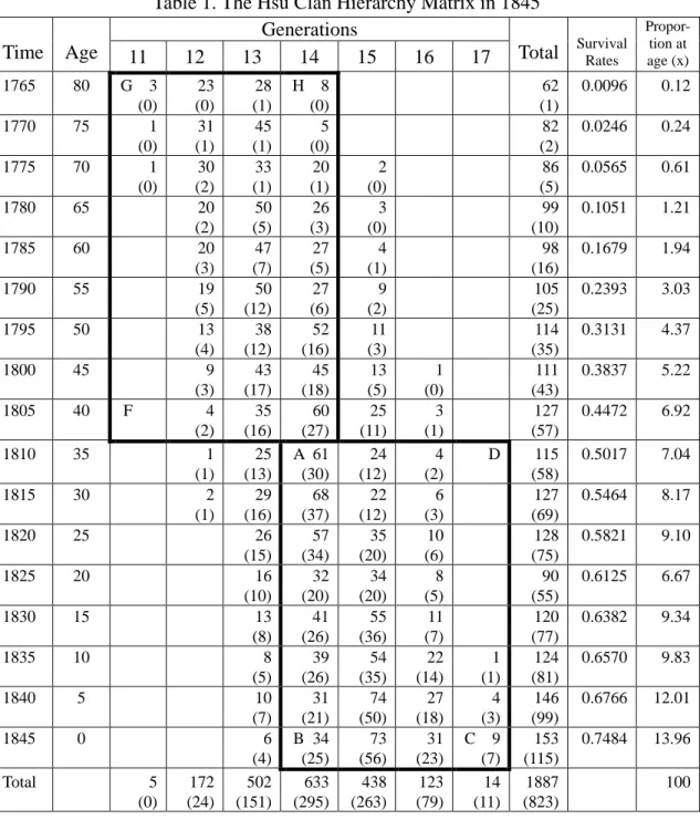
A typical hierarchy matrix of a clan is illustrated in Table 1 by that of the Hsü clan in the year 1845. The age and birth years are indicated by the row headings and the generational identifications are indicated by the column headings. The numbers
2
See Freedman, Lineage Organization, 33-40; H. W. Liu, Clan Rules, 14, for discussions on the clan hierarchy and size. Their integration into a hierarchy matrix for empirical implementation has, to our knowledge, never been attempted.
3
shown in each cell of this table indicate the numbers of male births and the numbers in parentheses for the males survived for each age and generational stratification.
Table 1. The Hsü Clan Hierarchy Matrix in 1845
Time Age
Generations
Total Survival Rates
Propor- tion at age (x) 11 12 13 14 15 16 17 1765 80 G 3 (0) 23 (0) 28 (1) H 8 (0) 62 (1) 0.0096 0.12 1770 75 1 (0) 31 (1) 45 (1) 5 (0) 82 (2) 0.0246 0.24 1775 70 1 (0) 30 (2) 33 (1) 20 (1) 2 (0) 86 (5) 0.0565 0.61 1780 65 20 (2) 50 (5) 26 (3) 3 (0) 99 (10) 0.1051 1.21 1785 60 20 (3) 47 (7) 27 (5) 4 (1) 98 (16) 0.1679 1.94 1790 55 19 (5) 50 (12) 27 (6) 9 (2) 105 (25) 0.2393 3.03 1795 50 13 (4) 38 (12) 52 (16) 11 (3) 114 (35) 0.3131 4.37 1800 45 9 (3) 43 (17) 45 (18) 13 (5) 1 (0) 111 (43) 0.3837 5.22 1805 40 F 4 (2) 35 (16) 60 (27) 25 (11) 3 (1) 127 (57) 0.4472 6.92 1810 35 1 (1) 25 (13) A 61 (30) 24 (12) 4 (2) D 115 (58) 0.5017 7.04 1815 30 2 (1) 29 (16) 68 (37) 22 (12) 6 (3) 127 (69) 0.5464 8.17 1820 25 26 (15) 57 (34) 35 (20) 10 (6) 128 (75) 0.5821 9.10 1825 20 16 (10) 32 (20) 34 (20) 8 (5) 90 (55) 0.6125 6.67 1830 15 13 (8) 41 (26) 55 (36) 11 (7) 120 (77) 0.6382 9.34 1835 10 8 (5) 39 (26) 54 (35) 22 (14) 1 (1) 124 (81) 0.6570 9.83 1840 5 10 (7) 31 (21) 74 (50) 27 (18) 4 (3) 146 (99) 0.6766 12.01 1845 0 6 (4) B 34 (25) 73 (56) 31 (23) C 9 (7) 153 (115) 0.7484 13.96 Total 5 (0) 172 (24) 502 (151) 633 (295) 438 (263) 123 (79) 14 (11) 1887 (823) 100
The hierarchy matrix portrays two-way ordering of member status under the clan system. A person generally has highly clan status if he belongs to an earlier generation and/or is older. For example, individuals in cell A have a higher (lower) status than those in the block ABCD (block AFGH). For certain ceremonial purposes the generational ordering takes precedence regardless of age (e.g., the listing of names in a funeral announcement or in ancestor worshiping), whereas the opposite is true in other clan-related functions (e.g., education and assignment of duty).
4
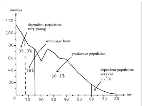
Figure 1a: Age Distribution of Clan Population
Figure 1b: Distribution of Clan Population by generation Identity
The age composition of the male population in this matrix is illustrated in Figure 1a. The declining property of this curve shows that the population pyramid of a clan is similar to that of the society as a whole as recognized by modern demographers. For example, the productive population (aged 15-59) is about 60 percent, whereas the dependent population (i.e., the very young and old) is about 40
5
percent. That the age structure of a clan is a mirror of that of the whole society suggests that the clan can function as a self-contained unit. With an appropriate age structure, the three basic economic functions of an agrarian society (production, rearing and education of the youth, and social security for the senior and needy members) can all be performed within the clan.3
The population distribution by generations of this clan is shown in Figure 1b. Its inversed u-shaped pattern indicates that there are relatively few members belonging to the older or the younger generations. These two figures imply a hierarchical structure in the sense that there are relatively few who are both old and belonging to the early generations. A distinct cultural trait of traditional China was that this venerable minority not only played leading roles in ceremonies but also constituted the authority of control at the top of the social pyramid.
THE GENERATION BIRTH SCHEDULES
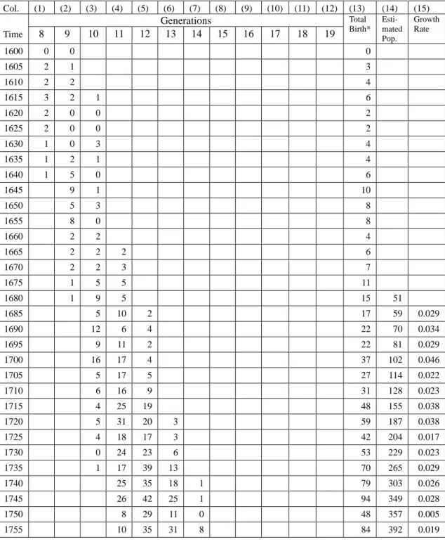
The generational birth schedules are constructed from the genealogies that recorded the birth dates of clan members stratified by generations. As an illustration of this procedure, the generational birth schedules of the males of the Hsü clan are first listed (see Table 2). The number in each column, indicating the number of mail births in each five-year interval (with the mid-year indicated on the first column of the table), forms a birth schedule of a particular generation. The total number of male births in each interval for all generations is indicated in column.4
The hierarchy matrix in Table 1 can be derived from the generational birth schedules with the aid of demographic principles. Assuming that the male longevity is eighty years, the segment of birth schedules from 1765 to 1845 (i.e., with an age range of eighty years as blocked in Table 2) is reproduced in Table 1. These entries are multiplied by the survival rates to deduce the hierarchy matrix previously discussed.5
3
The proportions of the three broad age groups in a stable population (model west, level 7 with R = 10) are 36.68%, 57.74%, and 5.57% respectively. See Ansley J. Coale and Paul Demeny, Regional Model Life Tables and Stable Populations (Princeton, 1960), 134. The age structure of the Hsü clan in 1845 was quite close to this model. Notice that in Figure 1a, there is a dent in the curve around age 20. This merely reflects the dent of the curve of observed male births around the year 1825. The well-known Confucian ideal of social order – the age of Grand Unity (ta-t’ung 大同) – already expressed that these basic economic functions be performed by a society. See Li Chi 禮記 (Book of Rites), section 9; for an English translation of this section, see William Theodore de Bary et al., Source of Chinese Tradition (New York, 1960), 175-176.
4
An investigation of 16 clan genealogies (including the 10 used in this article) see Ts’ui-jung Liu, “The Demographic Dynamics of Some Clans in the Lower Yangtze Area, c. 1400-1900,” paper presented at the International Conference on Sinology (Taipei, 1980).
5
The survival rates are the Lx/5l0 values in the life table. See Appendix 2 for an example of the life
table of the Hsü clan. For estimating the child mortality rates, two Princeton tables of model west levels 7 and 8 are used, see Coal and Demeny, Regional Model Life Tables.
6
From the hierarchy matrix we can readily calculated the total male population size as listed in column (14) of Table 2. From the population size we know the time path of the growth of the clan. The rates of growth are given in column (15) of Table 2.6
Table 2. The Generation Birth Schedules, Estimated Male Population and Growth Rate of the Hsü Clan in Hsiao-shan
Col. (1) (2) (3) (4) (5) (6) (7) (8) (9) (10) (11) (12) (13) (14) (15) Time Generations Total Birth* Esti- mated Pop. Growth Rate 8 9 10 11 12 13 14 15 16 17 18 19 1600 0 0 0 1605 2 1 3 1610 2 2 4 1615 3 2 1 6 1620 2 0 0 2 1625 2 0 0 2 1630 1 0 3 4 1635 1 2 1 4 1640 1 5 0 6 1645 9 1 10 1650 5 3 8 1655 8 0 8 1660 2 2 4 1665 2 2 2 6 1670 2 2 3 7 1675 1 5 5 11 1680 1 9 5 15 51 1685 5 10 2 17 59 0.029 1690 12 6 4 22 70 0.034 1695 9 11 2 22 81 0.029 1700 16 17 4 37 102 0.046 1705 5 17 5 27 114 0.022 1710 6 16 9 31 128 0.023 1715 4 25 19 48 155 0.038 1720 5 31 20 3 59 187 0.038 1725 4 18 17 3 42 204 0.017 1730 0 24 23 6 53 229 0.023 1735 1 17 39 13 70 265 0.029 1740 25 35 18 1 79 303 0.026 1745 26 42 25 1 94 349 0.028 1750 8 29 11 0 48 357 0.005 1755 10 35 31 8 84 392 0.019 6
7
Table 2 (continued)
Col. (1) (2) (3) (4) (5) (6) (7) (8) (9) (10) (11) (12) (13) (14) (15) Time
Number of male births in generations Total
Birth* Esti- mated Pop. Growth Rate 8 9 10 11 12 13 14 15 16 17 18 19 1760 3 22 35 9 69 410 0.009 1765 3 23 28 8 62 422 0.011 1770 1 31 45 5 82 445 0.011 1775 1 30 33 20 2 86 468 0.012 1780 20 50 26 3 99 497 0.019 1785 20 47 27 4 98 521 0.010 1790 19 50 27 9 105 548 0.010 1795 13 38 52 11 114 579 0.011 1800 9 43 45 13 1 111 604 0.008 1805 4 35 60 25 3 127 640 0.012 1810 1 25 61 24 4 115 663 0.007 1815 2 29 68 22 6 127 694 0.009 1820 26 57 35 10 128 723 0.008 1825 16 32 34 8 90 721 -0.001 1830 13 41 55 11 120 741 0.005 1835 8 39 54 22 1 124 759 0.005 1840 10 31 74 27 4 146 791 0.008 1845 6 34 73 31 9 153 823 0.008 1850 2 13 44 35 3 97 809 -0.003 1855 2 20 51 32 8 113 809 0 1860 9 20 36 6 71 776 -0.008 1865 4 18 45 5 72 744 -0.008 1870 9 21 27 15 2 74 715 -0.008 1875 8 19 42 16 2 87 695 -0.006 1880 2 21 53 22 2 100 685 -0.003 1885 5 15 46 26 6 98 673 -0.003 1890 2 15 43 35 11 105 667 -0.002 1895 16 29 33 11 89 651 -0.005 1900 10 21 36 11 78 628 -0.007 1905 7 29 54 27 4 121 642 0.004 1910 8 17 30 16 1 72 Total 15 42 96 284 479 651 724 703 577 303 88 5
*In the period 1600-1735, the number included the births observed for the eighth, ninth, and tenth generations for which the genealogical record was rather incomplete.
THE CLAN POPULATION SIZE AND EXOGENOUS DISTURBANCES
The columns (13) to (15) of Table 2 are represented by three curves in Figure 2. From these curves we can first isolate the exogenous influences. The growth of Hsü clan through two centuries (1700-1900) was interrupted by certain major exogenous events, i.e., natural calamities and wars (indicated in Figure 2). Two quite independent
8
sources of data, the clan genealogies and local gazetteers, are used to study this phenomenon. The consistency of these two data sources assures us of the reliability of both.
Figure 2: Hsiao-shan Hsü Clan
In Figure 2, the curve of “observed total male births” reflects two major interruptions: (1) between 1745 and 1765 and (2) between 1820 and 1845. For the first case, the local gazetteer of Hsiao-shan recorded a major famine in 1748 such that, “even the grass roots and barks were exhausted as the source of food supply and people died of eating the kuan-yin 觀音earth which they dug up from the ground.” For the second case, the gazetteer stated that in 1820, “a major drought occurred between May and July and the river was dried to the bottom to be followed by a flood brought about by typhoon, so that nearly 80 percent of the county was inundated with no hope of an autumn harvest.” Even minor natural calamities were faithfully reflected by minor dips in the birth curve as indicated in Figure 2.7
The interference of an “idealized” and smooth growth path by exogenous disturbances can be established for all of the ten clans that we have studied in this
7
See Hsiao-shan hsien-chih kao 蕭山縣志稿 (The draft gazetteer of Hsiao-shan county, 1935), 5: 26-31, for the chronology of natural calamities that occurred during the Ch’ing period. The two quotations appear in 5: 27 and 5: 29.
9
article. The long history of China was repeatedly and frequently interrupted by such natural calamities that arrested population growth. Our study provides a good demonstration of this fact.
THE LIFE CYCLE OF THE CLAN
From the three curves in Figure 2, we can clearly identify two growth phases (before 1845) and the contraction phase (after 1845). The Hsü clan was in the contraction phase after 1845, as all the three curves declined absolutely.8
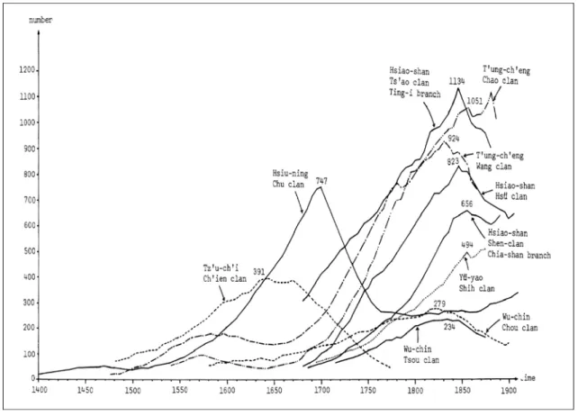
The inversed u-shaped population curve suggested that a clan begins to decline when its population size reaches a critical maximum value (CMV). This life pattern is in fact shown by all the ten clans covered in this study (see Figure 3). The average value of the peak clan (male) population of Figure 3 is 673. Our conjecture is that the CMV is an optimum value from a functional viewpoint – an issue that will be examined in the concluding section.
Figure 3: Estimated Male Population for Ten Clans in Chekiang, Kiangsu, and Anhwei
8
Due to the rather incomplete generational birth schedules prior to the twelfth generation, the total male births were underestimated before 1775 (the last birth of the eleventh generation). Hence, the growth process in the second half of the expansion phase was closer to the true situation.
10
STYLIZED FACTS OF THE GENERATIONAL BIRTH SCHEDULES
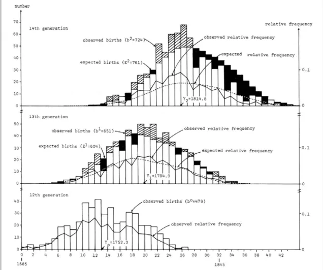
Before the CMV is reached, the growth of the clan is primarily a demographic phenomenon. To investigate this growth process, the generation birth schedules of the Hsü clan b0, b1, b2, … and their percentage distributions b*0, b*1, b*2… are represented by the bar diagrams and the solid curves in Figure 4, in which the horizontal axis represents the ancestor calendar. These diagrams show three stylized facts: an asymptotically bell-shaped curve, a constant mean gap, and a diminishing concentration tendency.9
Figure 4: The Generation Birth Schedules, Hsiao-shan Hsü Clan
For each bell-shaped generation birth schedule we can compute a mean birth year when a maximum value is reached (e.g., Y0 = 1752.3, Y1 = 1784.9, Y2 = 1814.8
9
Suppose x = (x1, x2, …, xn) is any row of numbers (i.e., a row vector), we shall use x* = (x*1, x*2,…,
x*n) = (x1/s, x2/s, …, xn/s) where s = x1 +x2 +…+xn to denote a “normalized” pattern of x. Thus, b*1 is
11
for the twelfth, thirteenth, and fourteenth generations of the Hsü clan). These birth schedules are asymtotically bell-shaped as members in the sequence b0, b1, b2, … become more regularly distributed in later generations. There are relatively few very old and very young male descendants for any generation. Obviously, the mean birth year gets larger for later generations (i.e., Y0 < Y1 < Y2 …). On a closer examination,
we find the mean gap (i.e., the difference between two consecutive means, Y i+1 –Yi,
such as Y1 – Y0 = 1784.9 – 1752.3 = 32.6 and Y2 – Y1 = 1814.8 – 1784.9 = 29.9)
appear to take on a constant value around thirty years, indicating a constant mean gap property.
Finally, we find that the birth range (i.e., the age difference between the oldest and youngest males) of a generation increases for later generations. Thus from Table 2, the birth ranges are 110 (= 1775 – 1665), 125 (= 1810 – 1685), 135 (= 1855 – 1720), and 150 (= 1890 – 1740) years for the eleventh, twelfth, thirteenth, and fourteenth generations respectively. This diminishing concentration tendency can also be seen from the fact that the b*t “bells” are getting shorted and wider for later generations, a property which can also be measured by the standard deviation of b*t.
These stylized facts which we have inductively established for the Hsü clan can also be established for all of the other clans examined in our article. The rigorously imply the structural characteristics of the hierarchy matrix (e.g., Figures 1a and 1b). The observed stylized facts are explained in terms of a demographic theory in the next two sections.
THE SINGLE ANCESTOR MODEL
To begin with our theoretical construction for the simplest case, it is natural to postulate the existence of single male ancestor E0, the starter of the clan. E0 will generate a “wave” of sons over time according to the male fertility schedule U1 = (u10,
u11…u18) (see Table 3). Thus, u1i (i = 0, 1, …8) is the probability that the spouse of a
typical father will give birth to a son by the time that the father’s age reaches the mid-point of the i-th age group in the following age groups: 15-19, 20-24, 25-29, 30-34, 35-39, 40-44, 45-49, 50-54, 55-59. In this way, the first generation E1 will be born.10
If every male in E1 again generates a “wave” of sons according to U1, the sum of all “waves” becomes E2 = (u20, u21…), the expected birth schedule of the second
generation. Recursively, the male ancestor generates a sequence of theoretically
10
For the concept of male fertility schedule (i.e., the net reproductive rate), see Henry S. Shryock et al., Methods and Materials of Demography (Washington, D.C., 1971), 541. What lies behind U1 are the age-specific fertility rates and survival rates. See Appendix 2 for the calculation.
12
expected birth schedules E1, E2,… for all future generations in the single ancestor model.
The demographic characteristics of the male fertility schedule that contains all information needed to generate the entire expected sequence of future generations can be described by five indices s1, τ, n, μ1, and σ21. First, the sum of all elements s1 =
1.413 is the total number of sons that ate expected to be born to a typical father during his lifetime.11 The magnitude of s1 governs the rapidity of growth of the clan in the
long run (see the discussion on the size of the clan above). Next, U1 specifies that a male before age fifteen cannot generate a son. Thus, τ = 3 (or 3 x 5 = 15 years) is the length of the non-productive period. Similarly, n = 9 (or 5 x 9 = 45 years) is the
productive period, or the maximum age difference between sons of the same father.12
From the “normalized” U1, to be denoted by U*1 = (u*10, u*11, …, u*1n-1) = (u10/s1,
u11/s1, … u1n-1/s1), we can define:
(i) a mean of U*1: μ1 = 0 u*10 + 1 u*11 + 2u*12 + … + (n – 1) u*1n-1 (μ1 = 3.187)
(ii) a variance of U*1: σ21 = Σ u*11 (i – μ1)2 (σ21 = 3.192)
Thus τ + μ1 = 3 + 3.187 = 6.187 (or 5 x 6.187 = 30.9 years) is the average fatherhood
of a typical father, which governs the mean gap between E1 and E i+1. The square root of σ21 is the standard deviation of U*1, that influences the degree of dispersion of the
expected birth schedules Ei. These intuitively obvious notions will be reflected in the content of the basic theorem stated below.13
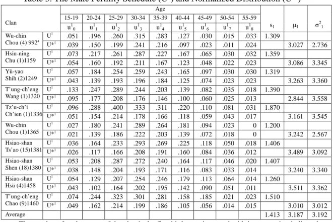
The parameter value of the male fertility schedule for the ten clan studies in this article are summarized in Table 3. Notice that every index shows the same order of magnitude for the ten clans, indicating that, during the period of traditional China, they are all governed by the same set of demographic forces.14
When a male fertility schedule U1 is given, we can predict the behavior of the expected birth schedules Ei according to the following theorem (proved as corollary 1 in Appendix 1). In this theorem, E*1 (i = 1, 2, 3 …) are the normalized “relative”
11
The numerical magnitudes cited in this section for illustration purposes are typical values, since they are the average of the ten clans listed in Table 3.
12
Intuitively, the productive period n governs the birth range of the expected birth schedules Et which is t (n – 1) + 1. For example, by the time of t = 72, the maximum age difference between the oldest and the youngest male descendants of “Confucius” in the seventy-second generation “could be” as high as 72 (45 – 1) + 1 + 3,169 years!
13 Imagine that the “age of father” is recorded on the birth certificate of every male child, then (τ + μ 1)
is the average “age of father” computed from a large number of such certificates. In our case, we were able to reconstruct more than 30% of families with birth dates of sons known from the genealogies.
14
The trend of s1, which is suppressed in this article, can be further explored to supplement the study
of Chinese population problems (e.g., fertility and mortality rates) in a historical perspective. See Ts’ui-jung Liu, “The Demographic Characteristics of Two Clans in Hsiao-shan, 1650-1850,” in Arthur P. Wolf and Susan B. Hanley (eds.), Historical Demography and Family History in East Asia, (forthcoming; note: it is published by Stanford, California: Stanford University Press, 1985).
13
frequencies of the expected birth schedules Ei (i = 1, 2, 3…). An ancestor calendar/ (instead of the Christian calendar) is used by taking the birth year of E0 (the ancestor) as the 0 year:
Table 3. The Male Fertility Schedule (U1) and Normalized Distribution (U*1)
Clan Age s1 μ1 σ21 15-19 20-24 25-29 30-34 35-39 40-44 45-49 50-54 55-59 u10 u 1 1 u 1 2 u 1 3 u 1 4 u 1 5 u 1 6 u 1 7 u 1 8 Wu-chin Chou (4) 992a U1 .051 .196 .260 .315 .283 .127 .030 .015 .033 1.309 U*1 .039 .150 .199 .241 .216 .097 .023 .011 .024 3.027 2.736 Hsiu-ning Chu (1)1159 U1 .073 .217 .261 .287 .227 .167 .065 .030 .032 1.359 U*1 .054 .160 .192 .211 .167 .123 .048 .022 .023 3.086 3.345 Yü-yao Shih (2)1249 U1 .057 .184 .254 .259 .243 .165 .097 .030 .030 1.319 U*1 .043 .139 .193 .196 .184 .125 .074 .023 .023 3.263 3.360 T’ung-ch’eng Wang (1)1320 U1 .133 .247 .289 .244 .203 .139 .082 .035 .018 1.390 U*1 .095 .177 .208 .176 .146 .100 .060 .025 .013 2.844 3.558 Tz’u-ch’i Ch’ien (1)1336 U1 .096 .288 .400 .333 .311 .220 .110 .081 .031 1.870 U*1 .051 .154 .214 .178 .166 .118 .059 .043 .017 3.161 3.545 Wu-chin Chou (1)1365 U1 .027 .180 .241 .289 .264 .181 .094 .023 0 1.200 U*1 .021 .139 .186 .222 .203 .139 .072 .018 0 3.242 2.567 Hsiao-shan Ts’ao (15)1381 U1 .036 .164 .233 .293 .269 .225 .118 .050 .018 1.406 U*1 .026 .117 .166 .208 .191 .160 .084 .036 .012 3.489 3.092 Hsiao-shan Shen (18)1380 U1 .053 .208 .287 .272 .240 .164 .117 .046 .020 1.407 U*1 .038 .148 .204 .193 .171 .116 .083 .033 .014 3.240 3.340 Hsiao-shan Hsü (4)1458 U1 .054 .129 .207 .254 .246 .179 .113 .064 .014 1.260 U*1 .043 .102 .164 .202 .195 .142 .090 .051 .011 3.511 3.362 T’ung-ch’eng Chao (9)1460 U1 .074 .244 .323 .301 .281 .158 .185 .021 .023 1.510 U*1 .049 .162 .214 .199 .186 .105 .056 .014 .015 3.010 3.012 Average 1.413 3.187 3.192
a. The number after the name of the clan is the first birth year in record with its generation indicated in the parenthesis.
Basic theorem: the sequence of relative frequencies E*1 of the expected
generation birth schedule Ei is asymptotically normally distributed, i.e., for large t, E*t is approximately distributed as
N (μE(t), σ2E(t)) where
μE(t) = t (τ + μ1) and (= 6.187t or 5 x 6.187t = 30.9 years)
σ2E(t) = tσ21 (= 3.192t)
are respectively the mean and the variance of a normal distribution.
This theorem can explain all of the stylized facts of Figure 4. First, the theorem not only predicts that the relative frequencies of the generational birth schedules (b*t) are bell-shaped, but is also predicts that they are approximately normally distribute. Furthermore, they become more “regular” for later generations. Next, the theorem states that the mean gap for two consecutive generations is μE(t + 1) - μE(t) = τ + μ1 or
30.9 years. Thus, the theorem not only predicts a constant mean gap but also tells us that the magnitude of this gap is precisely the average fatherhood age. Finally, the theorem predicts the diminishing concentration tendencies for Ei as the variances tσ21
14
increases for later generations. By giving plausible explanations to all the stylized facts, the basic theorem lends support to a demographical thesis underlying the formation of the clan.
THE MULTIPLE ANCESTOR MODEL
The clan as a Chinese institution in the pre-modern period is generally believed to have prevailed for some 800 years, beginning with the Sung dynasty. As pointed out by Freedman, the southeastern Chinese clans commonly extended to about twenty-five generations in the recent past. This is so because the constant mean gap of 5(τ + μ1) or 30.9 years implies a total of 773 years for twenty-five generations.15
For the study of such an antiquated institution, the lack of data for the early generations is an obvious impediment. The single ancestor model must be modified to accommodate the data deficiency. In a multiple ancestor model, a particular generation is first chosen as the ancestor generation, the birth schedule of which will be referred to as the ancestor birth schedule E0. All the males in E0, who are in fact distant cousins, will be interpreted as “ancestor.” A sequence of expected generation birth schedules E1, E2, … is generated from E0 when the same male fertility schedule is applied.
This theoretical procedure is illustrated by the Hsü clan in Figure 4. For the twelfth generation (i.e., the ancestor generation), there is one curve b*0 = E*0 which is the relative frequency of the ancestor birth schedule. There are two curves for each of the thirteenth and fourteenth generations. In addition to the observed sequence b*1 and b*2 (i.e., the solid curve), there is an expected sequence E*1 and E*2 (i.e., the dotted curve) which is the sequence of the recursively generated expected birth schedules. The primary data input of the multiple ancestor model is the pair (E0, U1). In addition to the five indices defined for U1 in the last section, there are four additional indices for the birth schedule of ancestor generation b0 = E0. The sum of all entries in b0 is sb0 = 479, the total number of male ancestors. The age difference between the
oldest and the youngest males in b0 is γ = 135, the ancestor birth range.
In the multiple ancestor model, it is natural to take the year in which the first ancestor was born as the 0 year of the ancestor calendar. (For the Hsü clan in Figure 4, the year 1685 is such a year and is the origin of the time axis.) To facilitate our exposition, we shall refer to b*0 = E*0 as a probability distribution function for an ancestor random variable x. In the ancestor calendar, x has a mean value μ0 = 13.46
15
H. W. Liu, Clan Rules, 7; Shimizu Morimitsu 清水盛光, Shina kazoku no kozo 支那家族の構造 (The structure of Chinese family and clan) (Tokyo, 1942), 215-228. Freedman, Lineage Organization, 6-7.
15
(or 5 x 13.46 = 67.3 years), the mean birth year of the ancestors, and a variance σ20 =
26.696. thus, altogether there is a total of nine indices s1, τ, n, μ1, σ21, sb0, γ, μ0, and
σ2
0 defined for the pair (E0 = b0, U1) in the multiple ancestor model. The following
theorem (proved as corollary 2 in Appendix 1) is a direct generalization of the basic theorem in the last section.16
Generalized Theorem: for large t, the relative frequency E*t is describable
approximately by the probability distribution function of a random variable zt = x + yt
where
(i) x is the ancestor random variable with mean μ0 and variance σ20
(ii) yt has a normal distribution N(μy, σ2y) where
μy = t(τ + μ1)
σ2y = tσ21
and hence the mean and variance of zt are given by (iii) μz(t) = μ0 + t(τ + μ1)
(mean: μz(t) = 13.46 + 6.51t)
σ2z(t) =σ20 + tσ21
(variance: σ2z(t) = 26.696 + 3.362t)
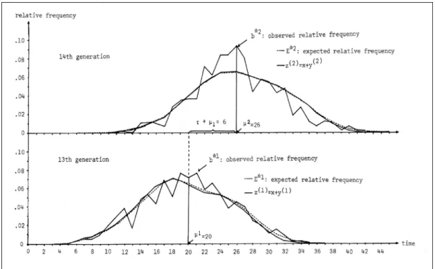
This theorem, which provides us with a method to approximate the recursively generated E*t by a well-defined function f(zt), is illustrated in Figure 5.
Figure 5: Observed, Expected, and Approximated Relative Frequencies
16
Note that if E0 = b0 contains precisely one ancestor, the multiple ancestor model reduces to the specific case of the single ancestor model.
16
For the thirteenth and fourteenth generations the b*t and E*t curves of Figure 4 are reproduced. For each generation, a third curve, corresponding to f(zt), is now added. Notice that E*t and f(zt) are, for all purposes, indistinguishable.17 To test our theory, we can compare b*t and f(zt).
Can f(zt) predict all the stylized facts? First, b*t is predicted to be bell-shaped, a slightly distorted normal distribution (see note 17). Moreover, the constant mean gap (τ + μ1), and the increasing variance (σ21) properties proved for the single ancestor
model, remain intact. Thus, the multiple ancestor model can be accepted. Six of the ten clans of Table 3 required the use of this model because of the data deficiency in early generations. The stylized facts are indeed verifiable for all of them. This testifies to the validity of the demographical approach.18
THE SIZE OF THE CLAN
To understand the clan as a self-contained socioeconomic function group, we should also theorize on the clan population size (see the section on the hierarchy matrix, above). As far as total male births are concerned, the basic theorem allows us to construct an expected sequence of generation birth schedules E1, E2, …. When they are tabulated as in Table 2, the sum of all columns denoted by E0 (= b0) + E1 + E2 +… is the expected total male births and is shown by the dotted curve in Figure 2. We have a clearer idea of the expansion and contraction of the clan by comparing the “observed” with the “expected” total male curves. When the clan was in the expansion phase (before 1845), the two curves follow the same time trend. In contrast, in the contraction phase (after 1845), the two curves clearly diverge as the expected total birth curve continues its increasing trend, while the observed total birth curve decreases through time. The turning point (1845) clearly marks off two phases of the life cycle of the clan. The total male population curve is inverse u-shaped and reaches the CMV at the turning point.
The demarcation of the two phases of the life cycle indicates that the formation and disintegration of the clan are governed by two distinct set of forces. What governs the expansion phase is basically a set of demographical forces. This is clearly shown by the coinciding pattern of the observed and expected total male birth curves. The
17
The immediacy of the nearly perfect approximation is amazing as the above theorem predicts a good approximation only for large t regardless of the shape of U1 or b0. The good approximation for
small t (i.e., for t = 1 and t = 2 corresponding to the thirteenth and fourteenth generations) is accounted for by two reasons. First, the male fertility schedule U1 is, itself, bell-shaped. Second, the ancestor birth schedule (or E*0 = b*0) is also bell-shaped as the basic theorem of the single ancestor model already predicts that b*0 should be bell-shaped – in fact, normally distributed.
18
17
divergence between them in the contraction phase reflects an entirely different set of forces, as is discussed in the next section.
One key analytical issue for the expansion phase is the rapidity in the formation of the clan. In the case of Hsü clan, it took 160 years (1685-1845) to grow to the CMV. Let sb0, sb1, sb2 … be the total male births of each generation (i.e., sbt is the sum of all
elements in bt in the multiple ancestor model). Obviously, sbt depends upon sb0 = 470
(i.e., the total number of ancestor in b0) and s1 = 1.26 (the total number of sons of a
typical father). In the multiple ancestor model, it is not difficult to prove the following theorem (Lemma 3 of Appendix 1).
Theorem 2: The total male births of the t-th generation is given by sbt = sb0st1.
Thus in the expansion phase, the generation population grows according to the rule of geometric progression.19
In addition to the growth of population by generations, we can also investigate the rapidity of growth of the total population via the use of modern demographical concepts. When the male fertility and mortality schedules are given, we can derive what is called the stable population growth rate (or the “intrinsic” growth rate) by solving a well-known equation.20 Using the data of the Hsü clan (see Appendix 2), the intrinsic growth rate is computed as r = 0.007 and is shown by the horizontal line in Figure 2. It is that growth rate of the total clan population that prevails in the long run. This growth rate applies only in the expansion phase. In this phase, the observed growth rate first decelerates toward and then fluctuates above the intrinsic growth rate. (In the contraction phase, the observed growth rate falls below the intrinsic growth rate.)
THE DISINTEGRATION OF THE CLAN
From its beginning in the Sung period, the institution of Chinese clan finally disintegrated toward the latter half of the nineteenth century. From Figure 3 we see clearly that the year 1850 was the turning point when most of the clans which we have studied began to decline, never to revive again. Although the Taiping rebellion might have been a contributory cause, their simultaneous disintegration signifies the termination of a long epoch which had existed in China for some 800 years.
19
According to this formula, the expected total births are 604 and 761 for the thirteenth and fourteenth generation respectively. The expected birth schedules are represented by the bar diagrams superimposed on those of the observed total births in Figure 4. The amount that the latter fall short of (exceed) the former is represented by the shaded (“crossed”) area. After the turning point (1845), the shaded areas predominate. This is again an indication that the clan had begun to disintegrate.
20 The equation is ∫w
0 e-ra p(a)m(a)da = 1. See Coale and Demeny, Regional Life Tables, 9-10, for a
brief discussion on A. J. Lotka’s original idea of stable population. Also see Shryock et al., Methods and Materials of Demography, 528, for the methods of calculation.
18
The Sung period heralded not only the beginning of the epoch of clan institution but also the development of the art of local government and the market system in traditional China. These new developments thus limited the functions to be performed by the clan in educating and rearing the youth, providing social security for the seniors and needy members, arbitrating minor disputes, and performing certain ceremonial functions.21
The termination of the long epoch of clan institution is an issue which should be separated from the life cycle of individual clans within this epoch. For example, in Figure 3, the Ch’ien clan and the Chu clan reached their peaks in 1640 and 1700, respectively, as they went through their individual and non-coinciding life cycles. To search for causes of the formation and disintegration of individual clans, we should emphasize their scale economy and diseconomy relative to the socioeconomic functions that they were expected to perform within the epoch.22
The clan was a space-sensitive social group. A precondition for the performance of all its functions was that its members have direct personal contact with one another. Because of the rather primitive means of communication and transportation in a pre-modern society, members of a clan could not live far apart (i.e., to satisfy the unilocal property). The primary school sponsored by the clan had to be attended by all school-age children. Members of the clan had to attend ceremonies at individual houses or at the clan temple. A dispute had to be quickly brought to the attention of the clan authority. All of these functions involved personal contacts within walking distance.
When the clan membership had grown to the critical maximum size (CMV) of about 700 males or 1,400 males and females, the clan would have contained any- where from 200 to 300 families. The execution of all of the clan functions was still quite manageable. For example, when the Hsü clan male population reached the peak value of 823, the number of school-age boys (according to Figure 1a) would have been around 130, all of whom could still have been accommodated on one centrally located school, even if everyone had chosen to attend the school. Conversely, the settlement of even a minor dispute would have taxed the capacity of the clan authority when the number of families was much larger than 300 or 400. The socioeconomic
21
For studies on the art of local government see, for example, James T. C. Liu, “The Sung Views on the Control of Government Clerks,” Journal of Economic and Social History of the Orient, X (1967), 317-344. For the development of the market system see, for example, G. William Skinner, “Marketing and Social Structure in Rural China, Pt. II,” Journal of Asian Studies, XXIV (1965), 195-228.
22
The case of the Ch’ien clan was due to a specific way of recording in its genealogy and the case of the Chu clan was due to migration. For a detailed discussion, see Ts’ui-jung Liu, “Demographic Dynamics of some Clans in the Lower Yangtze Area.”
19
functions intrinsically determined the CMV that limited further expansion of the clan.23
After the CMV had been reached, the scale diseconomy was accentuated because members would have had to live far apart. In an agrarian economy, the expansion of the clan population necessitated a simultaneous expansion of the area of cultivation. To minimize the daily transportation time for agricultural production, the sites of residence of its farming households spread out centrifugally. This dispersion increased the difficulty of contact and communication and hence rendered the clan functions inoperable. After the CMV was reached, the clan disintegrated because its members were alienated as a result of the space sensitive pattern of population location required of agricultural production. This disintegration was inevitable even when the supply of land was “unlimited.”
In the long run, population pressure constituted a new dimension of the problem because of the shortage of land area in a particular locality. Thus, superimposed on the centrifugal movement of farming households was the long-distance emigration when the local supply of land was exhausted. Natural calamities periodically hastened this process; exodus members often never returned, for basic economic reasons, to the place where their ancestor was born. Consequently, the descendants of the emigrants would not be recorded in the genealogies. Thus, although the expansion of clan was governed by demographic forces when the land supply was still abundant, its disintegration was rendered inevitable by land shortage. The life cycle of the individual clan was governed by multiple causes.
Why should a clan have disintegrated once it reached the CMV? Why could it not have maintained an optimum size? A clan did not exist in a social vacuum; it assumed a social existence. Our conjecture is that a clan would have had to compete with other clans and families for the acquisition of land in a particular locality. Before the CMV was reached, a clan grew with vitality and enjoyed a competitive advantage in land acquisition because of the potential of its efficiency of large-scale production. After he CMV was reached, our functional argument implies that all families of a clan with a number of populations in excess of the CMV would have had to disaffiliate with the clan. Thus in the declining phase, of its life cycle, the clan lost its competitive strength in land acquisition, and hence it went backward when it could not go forward, much like a boat rowing upstream against a rapid current.
23
It has been pointed out by many scholars that the traditional Chinese families were mostly small-sized with an average of 5.5 persons. In the case of stem families, the estimated size was about 10 persons. See H. W. Liu, Clan Rules, 2-3.
20
Appendix 1
Single Ancestor Model
In this single ancestor model the clan is started by a single male ancestor (i.e., the zero generation), the birth year of which is treated as the 0 year of the ancestor calendar. Letting 0m = (0, 0, 0, …,0) be a row vector with m-zeros, the male fertility
schedule can be written as A1a) E1 = (0τ, U1) where
b) U1 = (u10, u11, u12, …, u1n-1) with
c) s1 = u10 + u11 +… + u11
where τ is the non-productive period, n the fertility range, and s1 the total number of
sons expected to be born to a typical father during his life time. Letting Et be the birth schedule of the t-th generation, we have A2a) Et = (0tτ, Ut) t = 1,2,…, where
b) Ut = (ut0, ut1, ut2, …, utt(n-1)) with
c) st = ut0 + ut0 + … + ut t(n-1).
Notice thatEt is defined in A1. For t ≥ 1, Et implies that the oldest (youngest) male is not expected to be born before (after) the tτ-th (t(τ + n – 1) + 1) year of the ancestor calendar. Thus the birth range of Et is t(n – 1) +1 years, and the total births of the t-th generation is st. When a row vector Xn = (x1, x2, …, xn) is given, we can define the
following matrix: x1, x2, x3, …., xn 0, 0, 0, …, 0 0, x1, x2, x3,…, xn 0, 0, …, 0 0, 0, x1, x2, x3,…, xn 0, …, 0 A3) R(m, Xn) = . . . . . . . . . . . . . . . . , 0 0, . . . , 0, x1, . . . .. xn
with m rows and m + n – 1 columns. In this notation, Ut+1 is related to (i.e., generated by) Ut as follows:
A4a) Ut+1 = Ut R(t) where b) R(t) = R(t(n – 1) + 1, U1).
Notice that Ut has same number of columns as R(t-1) which is ((t–1) (n–1) + 1) + n–1 = t(n – 1) + 1, i.e., the birth range of Et defined in A2b). We have the following
lemma:
Lemma 1: The sum of all elements in Ut (or Et) is st = st1 and the relative frequencies of Ut and Et are, respectively
21
b) E*t = (0tτ, U*t).
Proof: A5b follows from A2. Applying A4 recursively, we have Ut = U1 R(1) R(2), …., R(t-1).
Post multiplying both sides by the column vector (1,1, …, 1), we have st = st1
by A1c which implies A5a. QED.
A random variable x with a probability distribution function f(x) will be called “zero-rooted with a range n” if f(x) = 0 except for x = 0, 1, 2, …, n–1. For these n-distinct values of x, f(xa0 can be written in a vector form:
A6a) Px = (p0, p1, …., pn-1)
(i.e., f(x) = Px for x = 0, 1, …., n–1 )
b) p0 + p1 + … + pn-1 = 1
The mean μx and variance σ2x of x can be unambiguously defined.
We can interpret E*t and U*t in A5b as the probability distribution function of the zero-rooted random variable zt and St respectively with mean and variance
denoted by (μE(t), σ2E(t)) for zt and (μt, σ2t) for St. A5b implies zt = St + tτ and hence
A7a) μE(t) = μt + tτ
b) σ2E(t) = σ2t
For t = 1, μE(1) = μ1 + τ and σ21 are, respectively, the mean birth year and the variance
of the male fertility schedule E1. For t ≥ 1, μE(t) and σ2E(t) are, respectively, the mean
and variance of the birth schedule of the t-th generation in the ancestor calendar. We will need the following lemma:
Lemma 2: If the zero-rooted random variable x (similarly y) with a probability
distribution function Px = (x0, x1, …, xn-1) (similarly, Py = y0, y1, …, ym-1) with a mean
μx (μy) and variance σ2x (σ2y), then z = x + y is a zero-rooted random variable with a probability distribution function:
A8a) Pz = (z0, z1, …, zn+m-2) = PxR(n, Py) with
b) μz = μx + μy (mean of z) and
c) σ2z = σ2x + σ2y (variance of z).
Proof: A8bc are obvious. Notice that z has a range 0, 1, 2,…, n+m–2 and is thus a zero-rooted random variable. For any integer i satisfying 0 ≤ i ≤ n+m–2, zi = ∑xkyj
summation over k + j = i. In case m ≤ n, we have
x0yi + x1yi-1 +x2yi-2 + …+ xiy0 for i ≤ m ≤ n
zi = xi-nym + xi-n+1ym-1 +… + xiy0 for m < i ≤ n
xi-nym + xi-n+1ym-1 + … + xn-1yi-(m-1) for m ≤ n < i
In all cases, zi is the i-th element in the row vector PxR(n, Py). For n < m, the proof is
similar. QED.
22
Theorem 1: If x1, x2, … xt are independent and zero-rooted random samples from a population U*1, the sample sum St = x1 + x2 + … + xt is a zero-rooted random variable with a probability distribution function U*t such that:
A9a) μt = tμ1
b) σ2y = tσ21
Proof: A9ab are obvious. To prove the theorem inductively, for t = 1, St = x1 and
the theorem is true by definition. Suppose the theorem is proved for t, then St+1 = St +
xt+1. The inductive hypothesis and Lemma 2 imply St+1 has a probability distribution
function
U*tR(t(n – 1) + 1, U*1) = (1/st+11)UtRt by A4b) and Lemma 1
= (1/st+11)Ut+1 by A4a)
= U*t+1 by Lemma 1.
QED.
Substituting A9ab in A7ab, we have A10a) μE(t) = t(τ + μ1)
b) σ2E(t) = tσ21
where τ + μ1 is the mean birth age of the male fertility schedule U1. The central limit
theorem applied to Lemma 1 leads to the following corollary:
Corollary 1: For large t, E*t is approximately normally distributed N(μE(t),
σ2
E(t)) where the mean μE(t) and variance σ2E(t) are defined in A10ab.
This is the basic theorem of the single ancestor model.
Multiple Ancestor Model
For the multiple ancestor model, in addition to the male fertility schedule U1 defined in A1, we need the ancestor birth schedule:
A11a) b0 = (b00, b01, b02, …, b0γ+1) with
b) s0 = b00 + b01 + b02 +… + b0γ+1
where s0 is the total number of ancestors and where γ is the ancestor birth range.
Letting Et (t = 1, 2, 3,…) demote the birth schedule of the t-th generation, then A12a) Et = (0tτ, bt) where
b) bt = (bt0, bt1, bt2, …, btt(n-1)+γ-1) with
c) sbt = bt0 + bt1 + bt2 + … + btt(n-1)+ γ-1
This is because for the t-th generation the first (last) male is not expected to be born before (after) the tτ-th year (t(n-1)+ γ–1 year) in the ancestor calendar (i.e., the 0 year is now the birth year of the first male in b0). The sum of all elements in Et (or bt) is sbt,
the total birth of the t-th generation.
The b0i ancestor in b0 generates a birth schedule b0iUt for the t-th generation.
23
A13) bt = b0R(γ, Ut).
This leads to the following lemma”
Lemma 3: The total male births (i.e., the sum of all elements in Et or bt) is sbt =
s0st1 (for s1 defined in A1c) and the relative frequencies of b* and E* are
A14a) b*t = (1/sbt)b0R(γ, Ut) = b*0 R(γ, U*t)
b) E*t = (0tτ, b*t).
Proof: A14b follows from A12a. Post multiplying both sides of A14 by a column (1, 1, ..., 1) leads directly to sbt = s0st1 by lemma 1 (i.e., st = st1). QED.
This lemma involves four relative frequencies E*t, b*t, b*0, and U*t which may be interpreted as the probability distribution functions of four zero-rooted random variables zt, wt, x, and St with means and variances denoted by (μE(t), σ2E(t)), (μw(t),
σ2
w(t)), (μ0, σ20), and (μt, σ2t). A14b implies that zt= wt + tτ and hence
A15a) μE(t) = μw(t) + tτ
b) σ2E(t) = σ2w(t)
The relation between wt, x and St is covered by the following theorem:
Theorem 2: If wt, x and St are the zero-rooted random variables with probability distribution function b*t, b*0, and U*t, then wt = x + St and hence
A16a) μw(t) =μ0 +μt
b) σ2w(t) = σ20 +σ2t
Proof: applying Lemma 2 to the pair “x and St” then A14a implies the theorem
directly. QED.
Substituting A16ab in A15ab and making use of A9a, we have A18a) zt = wt + tτ = x + St + tτ or
b) zt = x + y where y = St + tτ
the central limit theorem implies that, for large t, y is approximately normally distributed . Thus we have
Corollary 2: For large t, the relative frequency E*t is distribute as the sum of
two random variable zt = x +y where x has the probability distribution b*0 (i.e.,
relative frequency of the ancestor birth schedule with a mean μ0 and variance σ20) and where y is approximately normally distributed with a mean t(τ + μ1) and variance tσ2t.
(The mean and variance of zt are defined in A17ab.)
This is the basic theorem of the multiple ancestor model.
Appendix 2
In this appendix, taking the Hsü clan as an example, we discuss the nature of the genealogical data and the method of computing the empirical values of the birth schedules and the male fertility schedule.
24
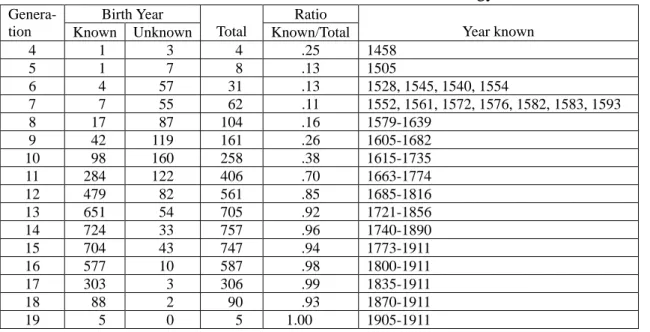
For the first three generations, the Hsü clan genealogy recorded only three names, without information on vital dates. From the fourth generation on, the record of vital dates can be found at first spottily and gradually more completely. Table A1 shows the number of males recorded by generations. These numbers and dates are the basic materials for our empirical evidence.
The generation birth schedules as shown in Table 2 of the text are derived by identifying he males in each generation according to their birth years at five-year intervals starting from 1600 (i.e., 1600 is the mid-point of the interval 1598-1602, etc.). The males whose birth years are not known are not taken into consideration in the construction of the birth schedules. As can be seen from Table A1, from the twelfth generation onward, the numbers with birth year known constitute well over 85 percent of the total; thus, the deleted unknown numbers may not cause great bias in our observation from the year 1685 onward.
Table A1: The Hsü Clan Male members Recorded in the Genealogy
Genera- tion Birth Year Total Ratio Year known Known Unknown Known/Total
4 1 3 4 .25 1458 5 1 7 8 .13 1505 6 4 57 31 .13 1528, 1545, 1540, 1554 7 7 55 62 .11 1552, 1561, 1572, 1576, 1582, 1583, 1593 8 17 87 104 .16 1579-1639 9 42 119 161 .26 1605-1682 10 98 160 258 .38 1615-1735 11 284 122 406 .70 1663-1774 12 479 82 561 .85 1685-1816 13 651 54 705 .92 1721-1856 14 724 33 757 .96 1740-1890 15 704 43 747 .94 1773-1911 16 577 10 587 .98 1800-1911 17 303 3 306 .99 1835-1911 18 88 2 90 .93 1870-1911 19 5 0 5 1.00 1905-1911
Since the male fertility schedule (U1) consists of two elements – the male age-specific fertility rates and mortality rates – each of them is discussed separately.
The male age-specific fertility rates were computed by applying the technique of family reconstitution to the genealogical data. On each family reconstitution sheet, the vital dates of parents and sons were recorded and the age differences between the father and sons were calculated. The fathers were grouped into five-year birth cohorts according to their birth years. The numbers of sons born to the fathers of the same cohort were distributed according to the ages of fathers in their reproductive period.
When we compute the age-specific fertility rates, the numerator is the aggregate number of sons born to the fathers at each age group and the denominator is the
25
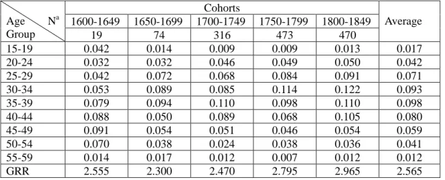
aggregate person-years spent by the fathers at each age group. Thus, the age-specific fertility rates of the cohorts of fathers can be obtained. Table A2 shows the male age – specific fertility rates computed from the data provided by the Hsü clan genealogy. In the text, the average value was used.
Table A2: The Age-specific Fertility Rates of the Males, Hsü Clan
Age Na Group Cohorts Average 1600-1649 1650-1699 1700-1749 1750-1799 1800-1849 19 74 316 473 470 15-19 0.042 0.014 0.009 0.009 0.013 0.017 20-24 0.032 0.032 0.046 0.049 0.050 0.042 25-29 0.042 0.072 0.068 0.084 0.091 0.071 30-34 0.053 0.089 0.085 0.114 0.122 0.093 35-39 0.079 0.094 0.110 0.098 0.110 0.098 40-44 0.088 0.050 0.089 0.068 0.105 0.080 45-49 0.091 0.054 0.051 0.046 0.054 0.059 50-54 0.070 0.038 0.024 0.038 0.036 0.041 55-59 0.014 0.017 0.012 0.007 0.012 0.012 GRR 2.555 2.300 2.470 2.795 2.965 2.565
a N denotes for number of families in observation.
GRR = Gross reproductive rate, i.e., the sum of age-specific fertility rates times 5.
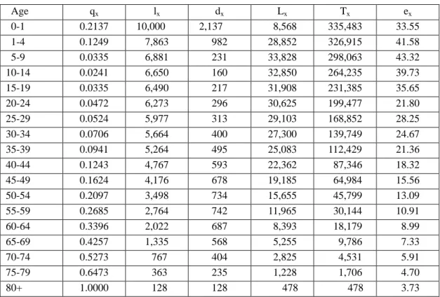
For computing the age-specific mortality rates, the technique if constructing a life table is applied to the genealogical data. Just as in the computation of the age-specific fertility rates, the males are first grouped into cohorts and then, according to their age at death, the age distribution of deaths for each cohort can be obtained. The number of deaths at each age group can be added up from the last age group to the first age group to obtain the number of survivors at each age group. The ratios derived from dividing the number of deaths by the number of survivors at each age group are the age-specific death rates. The observed death rates should be gradually for the purpose of constructing a life table.
In this study, all cohorts of the same clan are combined together to construct a life table. Table A3 shows, for example, a life table constructed for the males of the Hsü clan.
It should be noted that due to the nature of genealogical recording, the age-specific death rates of children under age fifteen cannot be derived directly because the information of child deaths is usually very incomplete.
In constructing a life table for all age groups, we have first constructed a life table of adults and then chosen two Princeton model life tables as references and extrapolated the observed values of death rates from the age fifteen down to age zero. This may not be the best solution for the estimates of the child mortality; however, a
26
better method for estimating the child mortality from the incomplete data of Chinese genealogies has yet to be devised.
For obtaining the male fertility schedule, the average age-specific fertility rates as shown in Table A2 are multiplied by the survival rates (i.e., the Lx/5‧l0 values in
the live table) at each age group and then multiplied by 5.
Table A3: Life Table of the Hsü Clan Males born 1600-1829
Age qx lx dx Lx Tx ex 0-1 0.2137 10,000 2,137 8,568 335,483 33.55 1-4 0.1249 7,863 982 28,852 326,915 41.58 5-9 0.0335 6,881 231 33,828 298,063 43.32 10-14 0.0241 6,650 160 32,850 264,235 39.73 15-19 0.0335 6,490 217 31,908 231,385 35.65 20-24 0.0472 6,273 296 30,625 199,477 21.80 25-29 0.0524 5,977 313 29,103 168,852 28.25 30-34 0.0706 5,664 400 27,300 139,749 24.67 35-39 0.0941 5,264 495 25,083 112,429 21.36 40-44 0.1243 4,767 593 22,362 87,346 18.32 45-49 0.1624 4,176 678 19,185 64,984 15.56 50-54 0.2097 3,498 734 15,655 45,799 13.09 55-59 0.2685 2,764 742 11,965 30,144 10.91 60-64 0.3396 2,022 687 8,393 18,179 8.99 65-69 0.4257 1,335 568 5,255 9,786 7.33 70-74 0.5273 767 404 2,825 4,531 5.91 75-79 0.6473 363 235 1,228 1,706 4.70 80+ 1.0000 128 128 478 478 3.73 Notations:
qx :Probability at age x of dying before reaching x + n.
lx : Number of survivors at age x out of an original cohort of 10,000.
dx : Number of deaths between age x and x + n out of an original cohort of 10,000.
Lx : Number of person-years lived between age x and x + n by an original cohort of 10,000.
Tx : Number of person-years lived at age x and over by an original cohort of 10,000.
ex : Average number of years remaining to be lived (expectation of life ) at age x.
The genealogies used in this paper are as follows:24
1. Hsü clan: Hsiao-shan T’ang-wan Ching-t’ing Hsü-shih tsung-p’u 蕭山塘灣井亭 徐氏宗譜 (1911).
2. Shen Clan: Hsiao-shan Ch’ang-hsiang Shen-shih tsung-p’u 蕭山長巷沈氏宗譜 (1893)
3. Ts’ao clan: Hsiao-shan Shih-ts’un ts’ao-shih tsung-pu 蕭山史村曹氏宗譜(1880). 4. Shih clan: Yü-yao Shih-shih tsung-p’u 餘姚史氏宗譜(1914).
24
A detailed study on the demographic data of these genealogies can be found in Ts’ui-jung Liu, “Demographic Dynamics of some Clans in the Lower Yangtze Area.”
27
5. Ch’ien clan: Ch’ien-shih cheng-tsung-p’u 錢氏正宗譜 (manuscript).
6. Chou clan: Pi-ling Shih-li-p’ai Chou-shih tsung-p’u 毘陵十里牌周氏宗譜(1904). 7. Tsou clan: Pi-ling Tsou-chih tsung-p’u 毘陵鄒氏宗譜(1875).
8. Wang clan: T’ung-ch’eng Wang-shih tsung-p’u 桐城王氏宗譜(1866). 9. Chao clan: T’ung-ch’eng Chao-shih tsung-p’u 桐城趙氏宗譜(1883).