ENHANCING BRANCH-AND-BoUND METHOD FOR
STRUCTURAL QPTIMIZATION
By C. H.
Tseng,'
L.
W. Wang,2 and
S. F.
Ling
3ABSTRACT: The branch-and-bound method was originally developed to cope with difficulties caused by
dis-continuous design variables in linear programming. When the branch-an~-boundmethod is applied to solve nonlinear programming (NLP) problems with a large number of mixed discontinuous and continuous design variables. the slow rate of convergence becomes a major drawback of the method. In thIs study. a number of enhancements are proposed to speed up the rate of convergence of the conventIOnalbranch-an~~bound algorithm. Three NLP in the form of truss-design examplesar~tested to compare the capabilitIes and effIcIency of the proposed enhancements. Itis shown that of the five CrIterIa for arranglllg the orderIIIwhich the deSign
variables are branched. the criterion of maximum cost difference dramatically reduces the number of branch nodes. thereby reducing the total number of continuous-optimization runs executed. Moreover. neighboring search. a branching procedure restricted in the neighborhood of the contllluous optImum. IS proven to be
effective in speeding up the convergence. Investigation also shows that branching several deSign varIables simultaneously is not as efficient as sequentially branching one variable at a time. The proposed enhancements are incorporated along with a sequential quadratic programming algorithm mto a software package that IS
shown to be very useful in the optimal design of engineering structures.
INTRODUCTION
As computer technology advances. optimization is becom-ing a powerful tooJ in engineerbecom-ing design. In conventional optimization algorithms. complications such as nonlinear functions. multiple objective functions, and a large number of design variables have been dealt with successfully [see, for example. Arora (1989)J. Although continuous design varia-bles are usually assumed in conventional algorithms, discon-tinuous design variables are frequently encountered in prac-tical applications. Examples are the size of a set of standard components (discrete), the number of teeth of a gear (inte-ger). or a choice between different design options (zero-one). The capability to deal with discontinuous design variables via conventional nonlinear-programming (NLP) problem algo-rithms would be a major expansion of the applications of structural optimization.
To make use of well-established continuous-optimization algorithms. most discrete-optimization techniques are based on the assumption of transforming the discontinuous solution space into multiple continuous solution subspaces. The op-timization problems in each of these continuous subspaces are solved sequentially by imposing constraints on discrete-ness of the design variables. The optimal discrete solution is chosen from among the continuous solutions obtained (Gochet and Smeers 1979). In addition to application cases of the branch-and-bound method that have been reported in ref-erences (Siddall 1982: Gupta and Ravindran 1981: Lee 1983). a general algorithm for solving NLP problems with integer and discrete design variables is presented by Sandgren (1990). However. there is a major obstacle to applying this algorithm to problems with a large number of discontinuous design var-iables: it requires too many executions of the continuous-optimization scheme and thus is very time consuming (Tseng 'Prof.. Dep!. 01 Meeh. Engrg .. Na!. Chiao Tung Univ .. Hsinchu, Taiwan. Repuhlic 01 China.
'Grad. Student. Dep!. 01 Meeh. Engrg .. Na!. Chiao Tung Univ .. IIsinehu. Taiwan. Repuhlie 01 China.
'Assoc. Prof.. School 01 Mech. and Production Engrg .. Nanyang Teehnol. Univ .. Singapore.
Note. Assoeiale Editor: Jashir S. Arora. Discussion open until Oe-toher I. 1995. To extend the closing date one month. a written request must be filed with the ASCE Manager of Journals. The manuscript for this paper was submitted for review and possihle puhlication on June 17. 1992. This p,lper is part of the journal ofStructural Engineering. Vol. 121. No.5. M'IY. 1995.0ASCE, ISSN 0733-9445/'.l5/0005-0H31-0H37/ $2.00 + $.25 pe'r page'. Paper No. 4252.
and Wang 19X9). Hager and Balling (198H) have solved the discrete-variable optimization problem for the design of steel frames. The problem is first converted into a linear program-ming (LP) problem after the continuous-optimum solution is obtained. Then the LP problem is solved using the branch-and-bound method in the neighborhood of the continuous optimum. This approach enables the branch-and-bound method to solve large-scale discrete-optimization problems effec-tively. Generally speaking. a survey of the literature (Vanderplaats and Thanedar 1991) shows that little numerical experience in using the branch-and-bound method has been reported.
In this studv, a number of enhancements to the conven-tional branch-illld-bound method are proposed to reduce the number of executions of the continuous-optimization scheme. The effectiveness of the following are investigated: (I) Se-lected branching order of nodes; (2) seSe-lected branching order of design variables; (3) neighboring search in the subspace near the continuous optimum; and (4) modified branching algorithm itself to improve the efficiency of the branch-and-bound method. The objective is to maximize the efficiency of using the branch-and-bound method in solving large-scale discrete-optimization problems. The proposed enhancement are coded in IDESNC to be readily incorporated with a se-quential quadratic programming (SQP) algorithm in an op-timization program IDESIGN3.51 [a modified version of the package IDESIGN3.5 used for solving continuous-optimi-zation problems (Arora 1989)J. To evaluate and compare the numerical performance of the various enhancements pro-posed. we developed the software IDESNC to solve three typical truss-design problems.
METHODOLOGY
Branching Order of Nodes
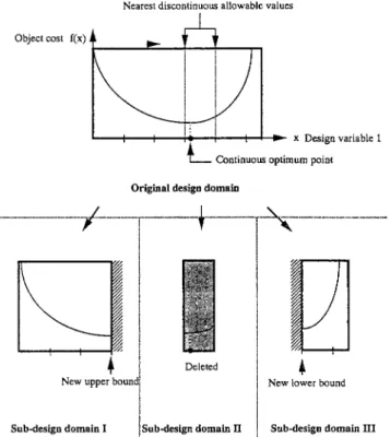
To locate a discrete optimum solution using continuous-optimization schemes, the branch-and-bound method re-peatedly deletes portions of the original design space that do not contain allowable values of the discontinuous design var-iables. This procedure is called "branching." First of all, the problem is solved by using a continuous-optimization algo-rithm. Ifthe continuous optimum occurs at an allowable dis-crete value for each of the design variables. the branching procedure should be stopped. Otherwise. the procedure should be continued. As illustrated in Fig. 1. the original design space JOURNAL OF STRUCTURAL ENGINEERING: MAY 1995,' 831
Nearest discontinuous allowable values Object cost f(x)
1---'=-...f--OO+---r-1
t:
i
! . x Design variable 1
L
Continuous optimum pointContinuous Optimum
Optimum (a)
Original design domain
Continuous Optimum
Optimum (b)
New lower bound Deleted
·--·-··---I--·----T---+·-·--r-~-·--···---·---EJ
I
II
~i
~ j~
I
• !New upper bound!
FIG. 1. Conceptual Layout of Branching Procedures
is divided into three subspaces with the allowable discontin-uous design values nearest the contindiscontin-uous-optimum solution as the upper and the lower bound of the left and the right subspaces, respectively. The center subspace, including the original continuous solution but excluding the feasible dis-continuous solution, is dropped. In each of the remaining two subspaces, the minimum cost may occur at a value of the design variable other than the newly assigned bound. A con-ventional continuous-optimization scheme has to be used again to find the optimum for each of the two remaining subspaces. If the new optimum does not occur at an allowable discrete value of the design variable in either of the subspaces, the foregoing branching procedure has to be repeated in each of the subspaces until a feasible optimal design is located. In the process, the combination of design subspaces always in-cludes all feasible discrete design variables, no matter how many levels of branching have been done. In addition, as the design space of the subproblem grows smaller, it becomes easier to identify the continuous solution in a subspace.
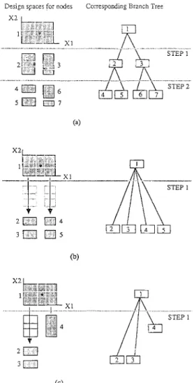
The "'tree" of the branch-and-bound method, i.e., a dia-gram of the branching, is shown in Fig. 2. Each design sub-space is depicted as a "'node." In principle, adi~cretesolution can be found if an exhaustive search of the tree is made. Conceptually, the exhaustive search can be either depth first or breadth first, as illustrated in Figs. 2(a and b), respectively. In a depth-first search, searching proceeds downward as far as possible before the search of another branch begins. In contrast, a breadth-first search proceeds one level at a time: one level is searched completely before descending to the next lower level. Both searching methods involve a large num-ber of continuous optimization and thus are very time-con-suming for the computer. Choosing an appropriate route in the tree so that the solution is reached more directly would drastically reduce the computing time required for the branch-and-bound method. Such a search route is depicted in Fig. 2(c).
In discrete optimization, the minimum cost in the original continuous design space is always less than or equal to that in the design subspaces that have been branched from the original space. This fact provides a guideline about when to
FIG. 3. Branching Order of Design Variables: (a) Minimum Clear-ance; (b) Maximum ClearClear-ance; (c) Minimum Clearance Difference; (d) Maximum Clearance Difference; (e) Maximum Cost Difference
COST 'u
tI
Optimum~f NodelI
x 3 1 ·
IJI
Assume optimum of Node2
I
COSlj, x31
•
..
~
+-+
+--l-x31•
x4I•
I
max x31•
x41•
-kJ-
-l---+
x31•
x4I•
W
~
(a)x2 1-1• •- - - i++
mm (b) x2 11-.---1I
-(e) x2 I-I• •- - - i (e) x2 I • I +---l-(d) x2 I • I+---l-~
Continuous Optimum l";-::; . .•.••0.
": 2 / '\,/~
3 /\, , c ... .t " Optimum (c)FIG. 2. Historical Diagrams of Searching Methods: (a) Depth-First Search; (b) Breadth-First Search; (c) Best-First Search
EX: f(x)=f(xl,
stop branching further in depth. If a feasible discontinuous solution is obtained in the process of branching, the corre-sponding cost-function value can be taken as a bound. Any other design subspace that possesses a continuous minimum cost larger than this bound need not be further branched, because further branching will only generate higher costs. This strategy is called "'bounding," and can be used to choose a branching route intelligently so as to avoid complete and impartial searching through the tree. The idea of bounding is useful only when the continuous-optimization scheme em-ployed yields the global minimum in each of the design sub-spaces. Theoretically, this is not always the case, because
Sub-design domain III
1
i
I
Sub-design domain II,
Sub-design domain I
832/ JOURNAL OF STRUCTURAL ENGINEERING / MAY 1995
whereXi = optimum value of the ith design variable; Xii and
Xi" = lower and upper allowable values of the ith design
variable, respectively;Llxi = smallest clearance of design
var-iablei; and X"h; = design variable to be branched.
2. Maximum Clearance: The criterion is the same as just
described except that the design variable with the maximum clearance is branched first. as follows:
Xl (b) 4
Design spaces for nodes Corresponding Branch Tree Xl
(a)
(I)
(2)
x"',, = min(.lx,. ,i,c' . . . ,.lx",)
.lx, = min(
lx, - X"I.lx, -
Xi"l) Branching Order of Design VariablesThe comments in last section concentrated on the branch-ing order of nodes for a sbranch-ingle design variable. When there are a large number of design variables, the order of design variables to be branched at the same node influences the efficiency of the method largely. In the following, we propose five different criteria to determine the priority in which the design variables are branched (Fig. 3).
I. Minimum Clearance: For each design variable, we
cal-culate the clearance between the nonallowable optimum point and the nearest allowable design value. The design variable possessing the minimum clearance is selected to be branched in the next step. The criterion is as follows:
there is no conventional optimization scheme that guarantees convergence to the global minimum except for the convex problems. Nevertheless, in the branch-and-bound method, the good news is that the possibility of converging to a global minimum increases enormously in practice because the same optimization problems are solved repeatedly in different de-sign subspaces with different initial guesses of dede-sign varia-bles.
4. Maximum Clearance DiHerence: This is the same as
cri-terion 3 except that the design variable with the maximum clearance difference is taken as the branch object, as follows:
x"", = max(.lCost" .lCostc... .lCost",.) (12) where Costiland Costi " = cost value of the lower and upper
bounds, respectively. of ith design variable at a node. and
(13)
I
iiI
I
.lCost, = ~(X", - Xii)
rix,
(e)
.lCosti = difference between the two costs. This criterion has
been used in Hager and Balling's 1988 paper.
The linear sensitivity coefficient,df"/dX" of the cost function at the optimum solution in the last higher level of the branch-ing tree can be used to estimate the cost difference between the lower and upper bounds of the ith design variable using the following equation:
FIG. 4. Conceptual Layout of Branching Algorithms: (a) Single Branch; (b) Multiple Branch; (c) Unbalanced Branch
Ifthis linear approximation is used tocalculate /lCost,. it is not necessary to use (9) and (10) to call the cost-function routine to evaluate the cost values. This :tpproximation thus greatly reduces the number of function calls.
In the first four criteria, the clearance between a continuous optimal point and its nearest discontinuous design point is taken as the criterion. By implication, the sensitivities of the cost function to all design variables are the same. This as-sumption makes evaluation and judgment fast and easy at the expense of accuracy. It is clear that the last criterion improves accuracy.
After a continuous-optimum solution is obtained at the first node, the algorithm searches through the subspace between
NB (a number of discrete value) larger and NBsmaller dis-crete values of each design variable out from the optimum to look for the discrete minimum. The value ofN Bcan be chosen Neighboring Search (3) (4) (5) (6) (7) (8) (9) ( 10) (11) ~ Xill~ .. ,XI/ •.) ,i" =
Ilx, -
x,,1 -
IXi - Xi"!
I
,i" =Ilx
i - Xiii -lx, -
Xi,,11 x"", = min(,i". ,i,c' . . . ..lx",,),i" = max(
lx, -
X"I.lxi - Xi,,!).lCost, = 'Costil - Cost,,,'
Cost" = f(x,. x, ..
Cost", = fIx,. x" .
3. Minimum Clearance Difference: This criterion is the
dif-ference between the clearances of the non allowable optimum point and the nearest lower and upper allowable values of each design variable. The design variable with the minimum clearance difference is taken as the branch object, as follows:
5. Maximum Cost Difference: At a node, we fix the values
of all design variables except one, and then evaluate the costs at the lower and upper bounds for the remaining variable. The design variable with the largest difference between these two costs is the branch object. as follows:
JOURNAL OF STRUCTURAL ENGINEERING: MAY 1995 833
~Continuous solution
o
Optimum solutionIIJIl
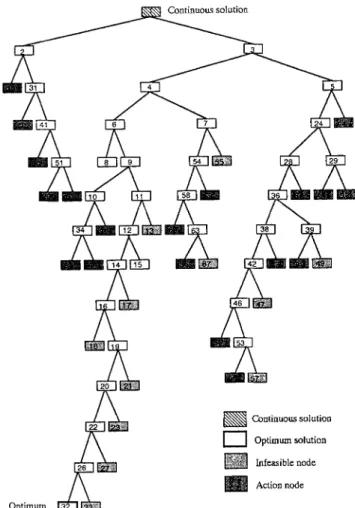
Infeasible node • Action nodeFIG. 5. Historical Diagram of Branching of 1O-Bar- Truss
Exam-ple
as one, two, or larger. For example,NB = 1 means that one bigger and one smaller discrete allowable values for each design variable in the neighborhood of the continuous opti-mum are taken as the subspace for searching in the remaining procedure. Ifsome design variables of the continuous opti-mum are right at the lowermost (or uppermost) discrete val-ues then the right (or left) subspace forN Blarger (or smaller) discrete values for that design variable are taken as neighbors. If N B = all in present paper, it means that all discrete values for each design variable in the original design space are used for the branching procedure.
Branching Algorithms
In branching algorithms; one node is always branched into two nodes in the next level in the tree, as shown in Fig. 4(a). If several design variables are dealt with simultaneously, the next level can be of more than two nodes. In this study, the following two new branching algorithms are proposed to im-prove the efficiency of the branch-and-bound method.
I. Multiple Branching: Fig. 4(b)for Multi-2 demonstrates
the idea of multiple branching using the case of two discon-tinuous design variables. For each of the variables, two sub-spaces are generated. Therefore, if the number of simulta-neously treated design variables isnforMulti-n, the number of nodes in one branching will be 2". Comparing Figs. 4(a and b) show that to achieve the same state of design subspaces in the next lower level of a tree, single-branching requires two steps of branching and 6 nodes in total produced, while the multi branching algorithm needs one step only with 4 nodes produced. Thus, in principle, multiple branching should be able to reduce the computing power required.
2. Unbalanced Branching: A conceptual layout of this
al-gorithm is illustrated in Fig. 4(c). This layout represents a compromise of the multiple-branching algorithm that avoids the disadvantages of complete and impartial branching. The algorithm can be thought of as a combination of the first and second steps of the single branching algorithm with one of the two nodes selected according to the concept of bounding.
NUMERICAL EXAMPLES
To investigate the performance of the foregoing methods, the branch-and-bound method with the proposed enhance-ments is incorporated with a SQP algorithm to solve three truss-diagram problems each with seven,
ro,
and 28 design variables, respectively. All three problems has been solved by Haug and Arora (1979), Thanedar et a!. (1986), and Arora and Tseng (1988) as continuous-optimization problems. The finite-element method is used for structural analysis. A hybrid design sensitivity method (Tseng and Kao 1989) that com-bines the advantages ofthe direct differentation method (DDM) and the adjoint variable method (A YM) is used to calculate the sensitivity coefficients. All the computations are done on an HP 835 workstation.1.JO-Member Cantilever Truss: The structure and its
load-ing is fully described in the case 11 of Example 4.5 by Haug and Arora (1979, page 242). The objective is to minimize the weight of the truss. The cross-sectional areas are taken as design variables. Nineteen constraints on stress, displace-ment, member buckling, and fundamental vibration fre-quency are imposed. The design formulation of the discrete-optimization problem is the same as that in the continuous case except the cross-sectional area of the truss members needs to be selected from the following set of discrete values: 1.62,1.80,1.99,2.13,2.38,2.62,2.63,2.88,2.93,3.09,3.13, 3.38,3.47,3.55, 3.63, 3.84, 3.87,3.88,4.18,4.22,4.49,4.59, 4.80, 4.97, 5.12, 5.74, 7.22, 7.97, 11.5, 13.5, 13.9, 14.2, 15.5, 16.0, 16.9, 18.8, 19.9, 22.0, 22.9, 26.5, 30.0, and 33.5. In practice, these discrete values may be those prescribed in the construction codes, e.g., the American Institute of Steel Con-struction (AISe) code.
Five criteria for the branching order of the design variables [(I) minimum clearance; (2) maximum clearance; (3) mini-mum clearance difference; (4) maximini-mum clearance differ-ence; and (5) maximum cost difference), four neighboring searches(NB = AlL 3, 2, and 1), and the three branching algorithms (single, multiple, and unbalanced) are tested. Table 1 shows the results of these studies and the comparable results given by Arora and Tseng (1988). The discontinous-optimum solution found by IDESNC is 0.9% better than that reported by Arora and Tseng (1988), which was only a guess solution obtained by the interactive capability of IDESIGN3.5. Fig. 5 is the tree diagram when the maximum-cost-difference cri-terion with NB = all is adopted. Altogether, there are 67 nodes and 442 function evaluations, and the cost-function value increases 0.33% as compared to the continuous opti-mum. Eleven nodes are deleted because they contained no feasible variable, and the first allowable discrete solution was obtained at node 32. The optimum cost value at this node was set as the bound for the nodes not yet branched, because they may possess optimum cost lower than the bound. The branching of each of the remaining nodes was terminated once an optimum was found that was larger than the estab-lished bound. This case took the central processing unit (CPU) approximately 20 times longer than the time required by the corresponding continuous optimization.
The results of the single branching and the maximum-cost-difference criterion with neighboring search for the number of discrete values(NB = 1,2,3, and all) are also shown in Table 1. The number of nodes and the function calls and the CPU time decreased when a smaller N B number was used.
TABLE 1 Summary of Results for 10-Bar- Truss Design Example
SINGLE BRANCH AND BOUND MULTI BRANCH AND BOUND
(1) (2) (3) (4) (5) Multi-2 Multi-3 Multi-4 Un-bala
Branch order of
design variables NB = all NB = 3 NB = 2 NB = 1
Number of nodes 471 101 275 X'J 67 53 43 5 105 205 12\ 'J'J
Funetion calls 3.725 6X2 2.0X4 5'JX 442 360 320 51 %3 1.727 1.113 1.076
Weight 5,431 5,414 5.414 5,415 5,414 5,414 5,414 5,4X'J 5,415 5,415 5,415 5,415
CPU time (see) 211.5 40.1 12'J.2 40.0 2'J.5 26.1 23.2 3.X 54.'J 102.'J 6X.5 4X.6
Oplimum SolutIOns Continuous design variabks I
I 2 I 3
I
4I
5 I 6 I 7I
X I 'JI
10 2X.27'J 1.620 27.261 13.727 1.620 4.0m 13.5'J5 17.544 1'J.130 1.62 Funetion ealls 22 Weight 5.3%.530CPU time (see) 1,4
Discontinuous discr<:tc I
I
2 1 3 I 4 I 5I
6I
7I
XI
'J I 10design variables" 30.00 2.62 26.50 13.'JO 1.62 2.62 13.50 IX.XO IX.XO 1.62
Weight 5,465.430
Weight increase('Ir ) 1.27
Discontinuous discrete I I 2 I 3
I
4 I 5 I 6 I 7 I XI
'J I 10design variahlcsb 30.00 I.XO 26.50 14.20 1.62 3.X4 13.'JO 16.'JO IX.XO 1.62
\Vcight 5,414.256
Weight increasl' (":' ) O.32X
CPU time (sec) 2'J.5
Note: 10 (discrcte) design variabks: I'Jconstraints: and420 (42 x 10)dIscrete values. "Arora and Tscng(I'JXX).
"IDESNC: NR = all.
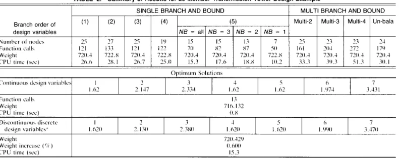
TABLE 2 Summary of Results for 25-Member Transmission-Tower Design Example
SINGLE BRANCH AND BOUND MULTIBRANCH AND BOUND
Branch order of (1 ) (2) (3) (4) (5) Multi-2 Multi-3 Multi-4 Un-bala
design variables NB = all NB =3 NB = 2 NB = 1
Number of nodes 25 27 25 I'J 15 15 13 7 25 23 23 24
Function calls 121 133 121 122 70 X2 X7 50 161 204 272 17'J
Weight 720,4 722.X 720.4 722.X 720,4 720,4 720,4 722.X 720.4 720.4 720.4 720.4
CPU time (sec) 26.6 2X.I 26.7 25.0 15.3 17.6 IX.X 10.2 33.3 3'J.3 5l.3 30.1
Optimum Solutions Continuous design variables 1
I 2 I 3
I
4 I 5 I 6I
7 1.62 2.147 2.334 1.62 1.62 1.'J74 3.431 Function calls 13 Weight 716.132CPU time (see) O.X
Discontinuous discr<:te I I 2 I 3
I
4 I 5 I 6 I 7design variabks" 1.620 2.130 2.3XO 1.620 1.620 I.'J'JO 3.470
Weight 720.42'J
Weight increase(r::, ) 0.600
CPU time (see) 15.3
Not<:: 7(discr<:te) design variabks:X7constraints: and2'J4 (42 x 7)discrete values. 'IDESNe: NR = all.
The final value of the cost function increased when NB was a small number because the subspace of neighbors about the continuous optimum was small. The neighboring search makes the process more efficient but not very accurate.
2. Bar Tower: The geometry and dimensions of a
25-member transmission tower are given by Haug and Arora (1979. page 245). Because of the symmetry of the structure and the use of the design-variable linking technique. seven design variables are used to represent the cross-sectional areas of the 25 truss members. There are '1:1,7 constraints imposed. The five criteria for the branching order of the design vari-ables. four neighboring searches. and the three branching algorithms are also tested. Table 2 shows the results of these investigations. The number of nodes decreased as smaller
NBs were used. However. the number of function calls and the CPU time increased for the cases when N B = 2 and 3 compared with that whereNB = all. Checking the procedure in detail shows that one of the branching nodes needed a larger number of function calls and iterations to obtain con-vergence in the SQP algorithm.
3. 200-Member Structure: To demonstrate the use of the
enhanced branch-and-bound method for large-scale prob-lems, a structure with 200 members, 77 joints. 150 degrees of freedom, and three independent loading conditions was selected as an example. The detailed design data of the struc-ture can be found in Haug and Arora (1979. page 250). De-sign-variable linking is used to represent the cross-sectional areas for 200 members in 29 design variables. The
optimi-JOURNAL OF STRUCTURAL ENGINEERING MAY 1995 835
TABLE 3. Summary of Results for 200-Bar 29-Design Variables Truss-Design Example
SINGLE BRANCH AND BOUND
Branch order of (1 ) (2) (3) (4) (5)
design variables NB = all NB = 3 NB = 2 NB = 1
Number of nodes 3,000' 3,000' 3,000+ IR7 131 59 49 13
Function calls 19,R05 ' 23,224 ' 19,30R+ 1,317 R59 512 347 59
Weight + + + 34.5R5 34,5R5 34,5R5 34,593 34,09R
CPU time (sec) 124,325 ' 147,100' 124,924 ' R,995,5 0,210.R 3,3R7.2 2,207.R 404.5
Optimum Solutions Continuous Design variables 1.020 1.020 1.020 1.020 1.020 1.020 1.020 2.27R 1020 3.27R 1.020 1.020 4.R37 1.020 5.R37 1.020 1.020 7,RoO 1.020 R.Rol 1.020 1.020 11.997 1.020 13.997 2.304 4.04R R.312 16.R27 Function calls 16 Weight 32,974.725
CPU time (sec) 174.R
Discontinuous"
Discrete design variables" 1.620 1.620 1.620 1.620 1.620 1.620 1.620 2.3RO 1.020 3.3RO
1.620 1.620 4.ROO 1.620 5.740 1.620 1.620 7.970 1.020 11.500
1.020 1.020 11.500 1.620 13.500 2.130 3.R40 11.500 15.500
Weight 34,5R5.147
Weight increasc(%) 4.RR4
CPU time (sec) 0,216.R
Note: 29 (discrete) design variables; 1.600 constraints; and I ,2IR (42 x 29) discrete values. "IDESNC;NB = all.
Object Cost
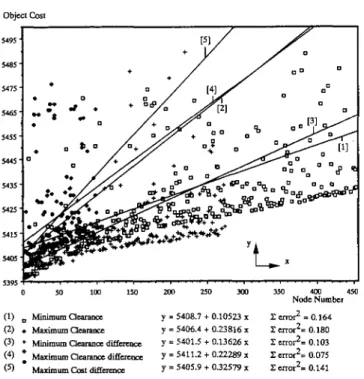
FIG. 6. Cost-increment Diagram of 1O-Bar- Truss Example
zation problems has 600 constraints in terms of member stress, nodal displacement, buckling, and the fundamental vibration frequency. Explicit design-variable bounds are also imposed. The formulation of this optimization is the same as that given in Haug and Arora (1979) and Arora and Tseng (1988) except that the design variables are discrete.
The continuous and discrete solutions are both listed in Table 3. The five criteria for the branching order of the design variables are again tested. When minimum clearance, maxi-mum clearance, and minimaxi-mum clearance difference are used as the criteria to determine the order of the branching design variables (cases 1 to 3), the solutions did not converge until the number of generated nodes reached 3,000. For the max-imum clearance difference and maxmax-imum cost difference
cri-Neighboring Search
If a discrete-optimum solution is near the continuous-op-timum solution or if the optimization problem is not highly nonlinear, N B allowable discrete values for each design var-iable in the neighborhood of the continuous-optimum
solu-COMMENTS
Branching Order of Design Variables
All five criteria proposed for determining the order in which the design variables are branched are tested for both the 10-member cantilever truss and the 25-bar-tower examples to compare their effectiveness in improving the efficiency of the branch-and-bound method. The results are shown in Tables 1 and 2. The rate of convergence and number of nodes created are significantly different. The criterion of maximum cost different performs best. This branching order promotes growth of the tree in depth rather than breadth, In Fig. 6, the cost-function values of the lO-member cantilever truss are plotted against the number of nodes for the five proposed criteria. The slopes of the best-fit lines indicate the rate of convergence of each criterion. The obvious difference in the slope of these lines indicates that the order of the branching design variable is the dominant criterion in determining the rate of conver-gence of the branch-and-bound method. As shown in Fig. 6, the criterion of maximum cost difference has the steepest slope and thus converges fastest.
teria (cases 4 and 5), however, only 187 nodes and 131 nodes, respectively, are generated in the process and the cost func-tion increases by only 4.9%. Although a large amount of CPU time is needed, the enhanced branch-and-bound method pro-vides a discrete-optimum solution.
The trend for the neighboring search is the same as that in the 10-bar-truss example. The number of nodes and func-tion calls and the CPU time decreased tremendously, and the final value of cost function increases slightly for the case in which NB = 1 compared with the case in which NB = all.
350 400 450 Node Numbe' 1: eno,2 = 0.164 1: erro,2= 0.180 1: erro,2= 0.103 1: erro,2= 0.075 1: erro,2= 0.141 300 250 200 y= 5408.7+0.10523 x y= 5406.4+0.23816 x y= 5401.5+0.13626 x y= 5411.2+0.22289 x y= 5405.9+0.32579 x ISO 100 50 (1) 0 Minimum Oearance (2) • Maximum Oearance (3) +Minimum Clearance difference (4) • Maximum Clearance difference: (5) MaximumCost difference 5415 5425 5435 5445 5455 5495 5465 5415 5485
8361JOURNAL OF STRUCTURAL ENGINEERING I MAY 1995
tion can be sought to obtain the discrete-optimum solution very efficiently and accurately. Iftpe problem does not fall into one of these categories. the value of N B must be in-creased to obtain a feasible solution. and the neighboring search becomes less efficient. In the results of the 25-bar-tower example. the number of function calls increases when the neighboring search is employed simply because a larger number of function calls and iterations is needed in the SQP algorithm. In practical usage for large-scale problems. it sug-gests the use of a smaller value ofN Bto obtain the value of the objective function in the beginning. Then a user can in-crease the value ofN Bto obtain the new value of the objective function. Ifthe new value of the objective function is con-verged. it can stop process for increasing the value of N B.
However. the value ofN B = all is still optional for the user to obtain the accurate solution if CPU time is accessible.
Branching Algorithms
The underlying concept of using alternative branching al-gorithms is to eliminate the middle nodes of a tree by allowing a branch of more than one design variable at a time. The proposed methods are applied to the lO-member cantilever truss and the 25-member transmission tower; the results are shown in Tables I and 2. The efficiency of the branch-and-bound method has not improved as expected.
To understand why. let us refer to Figs. 3(a and b) again. In multiple branching, one step of branching gives four nodes; however, these are different from and not as good as the four obtained by the two steps of the single branching. This is beeause the two algorithms use different information to select branching objects. In step two of single branching. new in-formation on the nodes obtained in the first step is used; in multiple branching. only the original information on the nodes is available to select the two branch objects in a single step. In single branching. sometimes one of the nodes generated in the first step will not be further branched in the second step, as illustrated in Fig. 3(a). In every step. one of the nodes may be abandoned, for reasons discussed previously. In mul-tiple branching. however. 2n nodes are generated directly
without providing the opportunity to check whether some of the nodes should be dropped. More nodes than necessary may be generated, thereby slowing down the rate of conver-gence of the solution process.
Unbalanced branching is proposed to overcome the afore-mentioned disadvantages of multiple branching. Test results show that it does improve the rate of convergence. Never-theless unbalanced branching cannot totally overcome the disadvantages of multiple branching, and the solution speed of this algorithm is slower than that of the single branching algorithm.
CONCLUSION
Third. single branch algorithm, which simplifies the branch tree the most, is more effective than the multiple and un-balanced branching algorithms for discrete optimization.
The software IDESNC, which combines the enhancements with the SQP optimization scheme. can be effective and ef-ficient in solving three structural-optimization problems in-volving discrete design variables. In the future. the problems of different scales (e.g., a larger number of design variables) and different types (mixed, discrete, and continuous) should be further investigated to make the branch-and-bound method more useful for solving engineering problems.
ACKNOWLEDGMENTS
The research reported in this paper was supported under a project sponsored by the National Science Council. Taiwan. Republic of China. grant number NSC7X-0401-E009-12.
APPENDIX I. REFERENCES
Arora. J. S. (l9X9). Inlrodllclion /() oplimal design. McGraw-HilI. New York. N.Y.
Arora. J. S.. and Tseng.C.H. (19X7). "I DESIGN: User's manual version 3.5." Tech. Rep. No. OD-X7.1. Optimal Des. Lab .. Coil. of Engrg .. Univ. of Iowa. Iowa City. Iowa.
Arora. J. S.. and Tseng.C.H. (19XX). "Interactive design optimization." Engrg. Oplimizalion.Vol. 13. 173-IXX.
Goehet. W.. and Smeers. Y. (1979). "A braneh-and-bound method for reverse geometric programming."Operalions Res ..27(5). 9X2-9%. Gupta. O. K ..and Ravindran. A. (19XI). "Nonlinear integer
program-ming and discrete optimization."Progress in engineering oplimiwlioll. R. W. Mayne andK. M. Ragsdcll. cds .. ASME. New York. N.Y. 27-32.
Hager.K ..and Balling. R. (ILJXX). "Ncw approach for diseretc structural optimization."J. Slrllc!. Engrg..ASCE. 114(5). 1120-1/34. Haug. E. J .. and Arora. J. S. (ILJ7LJ).Applied 0plimal design: mechallical
alld SlrllclUral syslems. John Wiley& Sons. Ncw York. N.Y. Lee. H. (ILJX3). "An application of integer and discretc optimization in
engineering design." MS thesis. Univ. of Missouri-Columbia. Colum-bia, Mo.
Sandgren. E. (l9LJ()). "Nonlinear integer and discretc programming in mechanical design."1. Meek Des.. Vol. 112.223-229.
Siddall. J. N. (l9X2). Oplimal engineerillg design: principles lind lIppli-calions. Marcel Dekker. New York. N.Y.
Thanedar. P. B.. Arora. J. S.. Tseng. C. H.. Lim. O. K.. dnd Park. G. J. (19X6). "Performance ofsomc SOP algorithms on structural design problems."Inl. 1. Numerical Melhods ill Engrg..Vol.2.\.2IX7-2203. Tseng.C. H.. and Kao. K. Y. (19X9). "Performance of a hybrid sensi-tivity analysis on structural dcsign problems."Compulers lind Sirucl .. 33(5).1125-1131.
Tseng.C.H.. and Wang.L.W. (ILJXLJ). "Thc application of branch-and-bound mcthod in largc number of non-continuous dcsign variables optimization."Tech. Rep ..Nat. Chiao Tung Univ .. Taiwan. Rcpublie of China.
Vanderplaats, G. N.. and Thanedar. P. B. (1991). "A survey ofdiscrctc variable optimization for structural design."Proc.. 10th COllI on Elec-Ironic CompUllllion in SlnK/. Engrg..ASCE. New York. N.Y.
APPENDIX II. NOTATION
The following symbols are lIsed in Ihispaper:
The following conclusions may be drawn from the numer-ical study presented here.
First, maximum cost difference. proposed by Hager and Balling (llJSS), is the most effective criterion among the five proposed criteria for determining the order of branching of the design variables.
Second. a modified branch-and-bound method with the capability of performing neighboring search is efficient but less accurate. The modified method is more suitable for solv-ing large-scale engineersolv-ing problems.
Costi" NB Xi' XiII X"h; 6.Cost, Illi
cost value of lower bounds of ith design variable at node:
cost value of upper bounds of ith design variable at node:
number used in neighboring search:
lower allowable values of ith design variable: upper allowable values of ith design variahle: design variable to be branched:
difference between two costs: and smallest clearance of design variable i.
JOURNAL OF STRUCTURAL ENGINEERING MAY 1995 837