NEW ALGORITHMS FOR THE LCS PROBLEM

JOURNAL OF COMPUTER AND SYSTEM SCIENCES 29, 133-152 (1984)

New Algorithms for the LCS Problem* w. J. Hsu AND M. w. Du

Institute of Computer Engineering,

National Chiao Tung University, Hsinchu, Taiwan, Republic of China

Received June 23, 1982; revised August 10, 1983

The LCS problem is to determine a longest common subsequence (LCS) of two symbol sequences. Two algorithms which improve two existing results, respectively, are presented. Let m, n be the lengths of the two input strings, with m Q n, p being the length of the LCS, and s

being the number of distinct symbols appearing in the two strings. It is shown that the first algorithm presented requires at most O(n log s) preprocessing time and O@m log(n/m) + pm) processing time to solve the problem. This bound is better than that of previous algorithms especially when n is much greater than m. The algorithm also exhibits desirable properties under conditions of sparse matches. The second scheme achieves essentially the same bound

(O@m log(n/p) + pm)) by employing efficient merging methods in the computations. It also

outperforms existing algorithms designed for sparsely-matched situations. Together, the two algorithms provide interesting contrasts of different approaches to one problem; they also offer improved alternatives for actual implementation. 0 1984 Academic Press, Inc.

I. INTRODUCTION

A string is a sequence of symbols. For computer manipulations, each of the symbols must be some representable information, such as an integer or an English letter. A subsequence of a string is obtained by deleting 0 or more (not necessarily consecutive) symbols from the string. For example, “aback’ is a string, and “bc&’ is a subsequence of it. A common subsequence (CS) of two strings, is a subsequence of both strings. A longest common subsequence (LCS) is one with the greatest length. For example, “top” is a CS of “entropy” and “topology”, while “topy” is the LCS of the two strings. Notice that, in general, two strings may possess more than one LCS. For example, both “abd” and “a&” are LCSs of “ubcd” and “ucbd.” The LCS problem is to find an LCS for two arbitrary input strings.

The LCS problem was first studied by molecular biologists [8, 9, 34, 361; they found a use for LCS in studying similar amino acids. Subsequently, together with other string problems, the complexity of the LCS problem was analyzed by many computer scientists (see the References), Other cited applications include data compression [2, 12, 281, pattern recognition [ 11, 271, etc., where the LCS of two strings is used as a certain similarity measure of the objects represented by the * This work was supported in part by the National Science Council of the Republic of China during the academic years 1980-1981.

133

t?Q22-0000184 $3.00 Copyright 8 1984 by Academic Press, Inc. All rights of reproduction in any form reserved.

strings. Closely related problems concern the computations of string-to-string distance (string editing) [26, 30, 41, 421, shortest common supersequences [ 12, 281, string merging [20], pattern matching [23, 321, and tree-to-tree distance [ 11, 371.

The algorithms presented here are actually improvements to two recent algorithms, respectively. So the closely related results that precede us are reviewed first, then followed by our algorithms. Since the LCS problem is well explored, properties that are already known are just pointed out and explained, rather than proved, to avoid unnecessary formalism. We do hope this approach evokes more intuitions and interests.

II. PREVIOUS RESULTS

We shall use A and B to denote the two input strings. Let IA I= m, IB / = n, without loss of generality, we assume that m < n. We also assume that the comparison of two symbols can be done in a constant amount of time, although a more realistic cost function should be logarithmic to the length of the codes. This assumption is still reasonable for almost every conceivable application.

The problem has been solved by using dynamic programming, e.g., [13, 35, 401. The idea is based on the following observation. Consider two strings A = u,u2 ... ai and B=b,b, -.a bj, if ai = bj, then by definition, an LCS of A and B must contain this coincident symbol as the last symbol; if ui # bj then the last symbol of an LCS can be either ui or bj (but cannot be both) or even neither. In this case, an LCS can still be obtained even if we drop the “redundant” symbol from the string containing it.

Let A[1 ... i] and B[l . ..j] denote the strings ala2 ... ui and b,b, ..a bj, and Li,j be the length of LCS of A [ 1 ... i] and B[ 1 -. a j]. By the above observations, we have

If ui = bj then Ll,jcLi-l,j-l + l

else Lo,j= maxlLt,j-l, Li-l,ji* We also have the following boundary conditions:

Li,o = 0 for i=O, 1,2 ,..., L,,j = 0 for j=O, 1, 2 ,...,

which simply means that the length of LCS of any string and a null string is zero. In [40], Wagner and Fischer employ an array L[O --. m, 0 +a. n] such that L/,j is kept in L[i,j]. With column 0 and row 0 of this array set to 0 initially, L[i,j] are computed row by row according to the above recursion. The desired value of L,,, is in L[m, n].

For example, A = abcdbb, B = cbucbuubu. After computing Li,j, the “L matrix” is shown in Fig. 1. Since row i (i > 0) of the L matrix corresponds to A [i], the ith symbol of A, and column j corresponds to B[j], the corresponding symbols were

THE LONGEST COMMON SUBSEQUENCE B c b a c b a a b a 012 3 4 5 6 7 8 9 0 0 0 0 0 0 0 0 0 0 0 a1000 ,111 11 b2 0 0 Ac3 0 2 2 2 d4 0 2 2 2 2 FIG. 1. L matrix. 135

shown. In this example, the length of LCS is in L[6,9], which is 4. Observe the regularity in Fig. 1; the region of (i - 1) is well separated from region (i + 1) by the region of i. We shall elaborate on this later.

Since we need to compute each of the m - n entries in the L matrix and computing each entry requires a constant amount of time, the total time required in computing the length of LCS is bounded by O(m - n), m, n being the lengths of the two strings. An LCS can be enumerated in O(m + n) time after computing the matrix, so the total time is bounded by O(m - n). The storage required in this algorithm is also bounded by O(m . n).

Hirschberg [ 131 improves the space complexity to O(m + n) by observing that in the calculation of Li,,, only Li_l,j_l, Li_l,j, and Li,j_l are relevant, i.e., row i does not depend on row (i - 2) or any other previous rows, hence row (i - 2) can be erased by now i without affecting the compution of row (i + 1) which again will erase row (i - 1). In all, only 2 rows, instead of m rows, are needed in the computation. Note that the time required is still O(m - n), since as many entries are computed.

As pointed out in [2], the straightforward dynamic programming algorithm for the LCS problem has the disadvantage that it takes the same quadratic amount of time on all inputs because they make no use of the inherent structures of the strings. Thus we prefer an algorithm which is more efficient for typical inputs.

In the foregoing approach, every entry in the m x n matrix is computed. To

develop algorithms that perform better than O(mn), we must reduce the number of entries to be considered. Observing that a CS is composed of only matched symbols, we have a chance. See the following example:

Given A = abcdbb, B = cbacbaaba, Fig. 2(a) shows an * on (i,j), whenever A [i] = B[j]. By this argument, we need only consider the *‘s on the diagram, instead of dealing with all the m X n entries.

Consider again the “L matrix” in a dynamic programming approach. Now with nonmatches abstracted away, see Fig. 2(b); since only matched symbols will constitute an LCS, if we can somehow compute the above Li,j values, we lose no

3c * *

4 d

5 b * * *

6 b t t ??

(a) points of matches

c b a c b a a b a

d

b

b

(b) reduced L matrix

FIG. 2. Matrices with reduced entries.

necessary information for computing an LCS. The regularity exhibited in the L matrix in the dynamic programming approach suggests useful structural property which might ease the computations.

In the following, we first examine how to represent the *‘s (the matches), then study the basic facts underlying each of the approaches. Two algorithms and our improvements are discussed subsequently.

Preprocessing

We may represent the points by keeping all the ordered pairs. For example, if A = acab, B = ababacb, the points are { (1, l), (1, 3), (1, 5), (2, 6), (3, I), (3,3),

(3,5), (4,2), (4,4), (4,7)}.

But the column/row regularity of the matches suggests better strategy. Specifically, we have the following property:

Let PB, = {j 1 (i,j) is a match] be the set of all positions in string B that match A[i], then PB, = PB, if and only ifA[s] =A[t].

So it s&ices to record a single copy of the set of j-values (positions in B) corresponding to each distinct symbol. See the following example.

THE LONGEST COMMON SUBSEQUENCE 137 EXAMPLE. For A = abcdbb, B = cbacbaaba, we may record the following infor- mation:

j-Values

e Coincident Positions in B N[iY]:

a 3, 6, 779 4

“e-lists” of String B b 2358 3

: 134 nil 0 2

Now, given A[ l] = a, we know, by inspection of the a list in the table, that (1,3), (1, ‘5), (1, 7), (13% are the matches on the first row of Fig. 2.

Similarly all other matches may be enumerated easily. To identify the coincident positions within a string is called a string identzj?cation problem in [2]. The known results may be used [14, 181.

We can set up the ‘Y-lists” for a string of length )2 in O(n log s) time, using O(n) space, where s is the total number of distinct symbols appearing in the string [ 141. Here a linear ordering of the symbols is assumed.

If the symbol set is known beforehand, this can be done even more efficiently by applying simple techniques, such as indexing-into-array, suggested in [2]. In this case, only O(n) time and O(n + l]Z[\) p s ace are needed. (]lZlj denotes the cardinality of the alphabet Z.)

In subsequent discussions, we assume that the e-lists are already provided. PB[O, 11, PB[B, 2],..., PB[O, N[fI]] is the ordered list of j-values (ascending) that correspond to 8.

Preliminary Facts

For convenience, an ordered pair (i,j) with A[i] = B[j] is now referred to as a “point,” and the value of ~5,,~ is called the rank of the point. Also, we would refer to the set of points that have the same rank as an “equipotential class”, or “class k’ (denoted C,), if K is the rank of the members; (0,O) constitutes class 0.

We now consider the regularity exhibited in the geometry of a class, then study the alternatives for determining the ranks of the points. For this purpose, we define a point (i,j) to be a successor of another point (i’,j’) iff i’ < i andj’ <j, which simply means that the symbol corresponding to the point (i’,j’) precedes the symbol corresponding to (i,j) in both strings. Clearly, any point which is a successor to a point P must have a higher rank than p; also, any point in class K (K > 1) must be a successor to some point in class (K - 1).

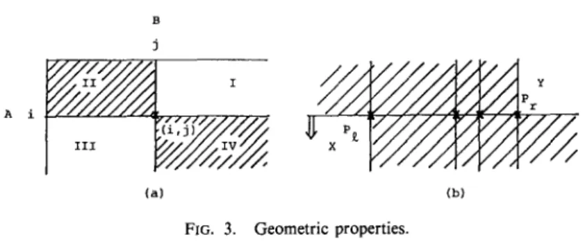
We may imagine that a point (i,j) divides the plane into four regions, as shown in Fig. 3a. Since (i,j) is a successor to any point in region II, any point in that region cannot be in the same class, otherwise (i,j) should have even greater rank. Similarly,

A i

(a) (b)

FIG. 3. Geometric properties.

points in region IV must be a successor to (i,j), so they must have higher ranks. The conclusion is, other members of the same class of (i,j), if they exist, must reside either in region I or in region III, or on the two axes (row i and column j).

Now suppose several class K points are known to be on the same row, as shown in Fig. 3(b). The leftmost point dictates that the region IV delineated by it (shadowed, under the row of points) cannot have any class K members; while the rightmost point also rules out the region II delineated by it. So the only regions left to be considered for class K are the unshadowed regions (X and Y) shown above. The above arguments apply to every row, hence the locations of points in the same class always shift to the left from row to row (cf. Fig. 2(b)).

Further, when determining a class, if we scan from row 1, row 2,..., in that sequence, with the upper portion being examined already, then only the lower-left region (region X in the above diagram) remains to be considered. The region X is completely determined by the leftmost point of this class considered so far, i.e., the position of this very point acts as a “threshold.” The vertical break lines on Fig. 2(b) correspond to the “thresholds.”

To closely correspond to the aforesaid ideas, we let C: denote the partially deter- mined class K associated with i, which is given by Ci z {(s, t) E C,, 0 < s < i}; and let Pk E min{j 1 (i,j) E Cl}, if CL # 0, to denote the “threshold” position of C, at i (the leftmost position of rank K points considered so far). As already mentioned, PL plays an important role in the determination of other class K members. We define

P: = co, if C: = 0. Clearly,

co =P;>P:>Pp:> *a* >P;: for any class C, (k > 0).

The above left-shifting property says that if (i,j) is in class K then j < Pi-‘. Moreover, Pk:‘, <j, since there must exist a point in class (K - l), so that (i,j) is its successor. It can be seen that the above argument is also reversible. Hence, we have

THEOREM 1. A point (i, j) is in class K, if and only if PL-_‘, < j < Pk- ‘.

In [ 141, Hirschberg also pointed out that instead of keeping all points of all ranks, a subset called the “minimal candidates” is sufficient in detrmining a single LCS.

A point (i, j) is a minimal K-candidate l@ PL-_‘, <j < Pk--’ and j= PL. (cf. Lemma 3 in [ 141).

THE LONGESTCOMMON SUBSEQUENCE 139 The “minimal candidates” are circled in Fig. 2(b). We shall refer to a “minimal K- candidate” as a “k-key”, for short. The above characterization says that (i, j) is a K-key, if and only if it is in class K; besides, it causes a change of the threshold position of the class. In Fig. 2(b) the keys are located at the corners of the “contours” [14]. It can be seen that each “contour” has at least one such turning point, i.e., if KEY(K) denotes the set of K-keys, then

KEY(K) = 0 iff C, = 0.

III. RECENT DEVELOPMENTS

Approach 1

The algorithm in [ 141 by Hirschberg is very efficient and deserves some detailed study. Actually, it would be impossible to appreciate the merits without going into the delicate points. Besides, our first algorithm is closely related to it.

His algorithm considers class 1, then class 2, class 3,..., in that sequence, until classes of higher ranks are found to be empty. In considering a class, the algorithm scans points on a row from right to left testing for the conditions in Theorem 1, then proceeds to the next row.

Hirschberg’s algorithm is based on the structural property that the locations of class K members on a given row are to the left side of all the class members in the last row. He avoids searching on the region that is bound to have no class K members.

He observes that if A [ill = A [i2] = 8, with il < i2, since Pi > PL > Pi > . . e > P{ ,

we must have Pi’ > Pi’-‘. Suppose that we are determining which points at row are members ofK&ssKK+r, we are finding (i2, j) with P$!I: <j & PF-‘;

i2 since Pi2-l < Pi1 a point (i2, j) with Pg <j need not be considered. Recall that all the p:ints’at ?ach row are kept in the order of (ascending) ‘(j-values,” i.e., if (i, jJ, (i, j,) ,..., (i, j,) are the points at row i, then the list j,, j, ,..., j, is kept by our preprocessing. Since A [ill = A [i2] = 0, the lists ofj-values corresponding to il and i2 actually coincide (cf. the discussion on preprocessing). So if at il, we register the greatest u with j, <P:, then, by the above argument, at row i2, we may just check the following list: j,, j,_, , jU_-2 ,..., and disregard the other part of the original j-value list. Note that the above upper limit (u) in the search for class K members applies only if A[il] and A[i2] contain the same symbol. So Hirschberg employs an array high [O] to register, for each distinct 8, the current upper bound of a search at a row containing 8.

The lower limit of serach for class K members at row i in Hirschberg’s algorithm is provided by P&_ll, which is also kept in an array.

It is precisely through such observations and arrangements, in Hirschberg’s algorithm, when identifying a class K that the j-values examined at row il need not be examined again at row i2 (il < i2, A[il] = A[i2] = 0) excepting thejp which joints

the two ranges of searches, The exact arrangements are much more complicated and are referred to the original paper.

Here is a simplified description of Hirschberg’s algorithm. PB[B, 11, PB [0, 2],..., PB[O, iV[O]] is the (ordered) list of all j-values corresponding to 8, which is provided by the preprocessing, KEY(K) denotes the set of K-keys, which is empty initially.

repeat

KtK+ 1; KEY(K)+& Pi+ CO; high[0] t N[B] for all 19,

For i c 1 to m do {Scan the points from right to left}. OtA[i],

while PB [ 0, high [ 01 ] > Pk- ’ Do high [ 01 + high [ 01 - 1; while Pi-_‘, < PB[O, high[f?]] Do Pi+-- PB[O, high[8]];

{Pi = min(j 1 (i,j) E Ci} high[f?] t high[B] - 1

IF Pk # Pk--’ then KEY(K) G (i, Pk) until KEY(K) = 4.

Since different 8’s occupy different positions in string B, the total number of allj- values canot exceed 1 BI, or n. Recall that at each row, when considering a class, only one j-value examined before is checked again, so the total number of j-values examined when considering a class can be bounded by (I B 1 t (A I), or (n + m), where 1 A 1, or m, accounts for the number of “overlapped” j-values examined at all rows.

Hence at most ~(m + n) j-values are examined for p classes. Since examining a point takes a constant amount of time, his algorithm takes at most O@(m t n)) time for comIjuting the ranks. Again, since m < n is assumed, so the time complexity is O(P).

Since only O(m) time is required for the postprocessing (to enumerate an LCS), we shall concentrate on improving the major part of the whole work.

Improvement

In Hirschberg’s algorithm, the lower bound for the determination of a K-key at a row, say row i, is set by the value of Pi:‘,. Essentially, the algorithm searches sequentially through the j-values that are located between the lower bound and the upper bound (high[e], if A[i] = 8). We propose an algorithm which preserves the same basic scheme (that avoids duplicated searches) but may benefit additionally from the power of binary searches.

First, we observe that a point cannot belong to more than one class, hence, for points that have been determined the ranks should not be considered again for higher ranks; rather, they should be “annihilated” in later computations. Since by Theorem 1, (i,j) E C,, if and only if Pk:ll <j < Pi-“, for all ranks and all rows. So

THE LONGEST COMMON SUBSEQUENCE 141 the points of lower ranks will always be annihilated from the left portion of a row. We use LOW[i] as an index to the smallest j-value remaining to be considered at row i.

Again, if A [i] = 19, we use HIGH[t9] to point to the greatest j-value to be considered at i. Note that, in the algorithm shown below, HIGH[A [i]] is set to keep the old LOW[i] (in Step 6.4). This fact is important in our following analysis.

THRESH, whose value is a function of i, denotes Pk-l, the threshold position of the class under consideration.

PB[B, 11, PB[R 21,..., PB]~,~]~]], as before, is the ordered list of j-values (produced by the preprocessing phase) that correspond to 13, N[B] being the number of Q’s in B.

With the above devises, for a class C, under consideration we iterate the following steps on i (1 < i < m) (cf. Step 6 of the Algorithm Al),

(1) Decide if there is a key of C, for this i. By Theorem 1, this can be done by checking PB[8, LOW [i]], which is the minimum j-value of the remaining points at this row, against Pi--’ (current THRESH). This is handled in 3 cases in Step 6.4.

Since it is possible that all points of a row are annihilated before-LOW [i] is set toN[A[i]]+l ( see next step). We will check, in Step 6.2, LOW[i] against N[A[i]], for the number of points in this row before using LOW as an index.

(2) Annihilate points, if any, that belong to C, by adjusting LOW[i]. By our definition of LOW[i], this can be done by finding t the greatest integer such that PB[A[i], t] < Pk-‘, i.e. t E max{l/ PB[A[i], l] < PL-l}, then setting LOW[i] to 1 + t. We denote the search of t by a procedure FIND (t, i, HIGH, LOW, THRESH). We shall show that t can be found between HIGH and LOW, i.e., LOW[i] <t < HIGH[8], where 0= A[i].

(3) Set Pk (new THRESH) according to the result of (1) (2).

ALGORITHM Al (A Variant of the Algorithm in [ 141). Only the improved portion is shown. The length of LCS can be determined by executing this algorithm.

Steps:

(0) LOW[i] +- 1 fori= 1 tom;

(1) KcO;

Repeat

(2) HIGH[A[i]] +N[A[i]] fori= ltom;

(3) KtK+ 1;

(4) KEY(K) c 0;

THRESH + 00; {‘.‘C~=~,P~=ao,K>O)

Fori= ltomdo

(6.2) IF LOW[i] < N[B] Begin (6.3) jtPB[& LOW[i]]; (6.4) Case 1. j > THRESH HIGH[8] t LOW[i]; Case 2. j= THRESH HIGH[f?] + LOW[i];

then Some points at this row remain to be considered

j is the minimum j-value at this i remaining to be con- sidered

j > Pi-l, by Theorem 1, none of the points at this row belongs to C,

Pi < PB [O, high[f?]] after this operation

j = Pk-‘, by Theorem 1, at this row, exactly one point belongs to C,

Hence, Pb = PB[t$ high[f?]] after this operation

LOW[i] c LOW(i] + 1; Delete this point from later considerations

Case 3. j < THRESH

KEY(K) c= (i, j);

j is the minimum j-value that has PL-;’ <j < Pk-‘l; :. (i,j) is a key, and Pk = j

FIND(t, i, LOW, HIGH, THRESH);

(trmax{lIPB[B,I]~P~-I}} THRESH e j; {Pk = min{ jl (i, j) E Ck}} HIGH[B] + LOW[i]; {Pb = PB[B, high[8]] after

this operation}

LOW[i]+t+ 1;

end{IF) end {For } until KEY(K) = 0;

p+-K- 1; number of all nontrivial classes, or equivalently, the length of LCS

next phase: {For generation of an LCS, see [ 14]}.

As can be noticed, the algorithm developed here essentially follows the same scheme of Hirschberg’s algorithm. The complete proof of correctness can be established in much the same manner [ 161 (basically, this requires Theorem 1 and the observations made earlier, coupled with some inductive arguments), hence is avoided. The operations done in Case 1 and Case 2 are quite simple, and can be verified

THE LONGEST COMMON SUBSEQUENCE 143

easily. The “FIND t” part in Case 3 needs some examination. Here we just show that t, the new LOW[i], can indeed be found between LOW[i] and HIGH[A[i]].

Consider the following facts:

(1) Obviously, LOW [i] < t; because PB [0, LOW [i] ] < Pi-l (Case 3), and t=max{l(PB[@Z] <Pi--‘}.

(2) Again, t < HIGH[A[i]]: Recall that HIGH[B] is initialized to N[B] in Step 2; if i is the first (smallest) such that A [i] = 19, then HIGH [0] provides a sure upper bound for t. If i is not the first such that A [i] = 8, i.e., there exists i’, i’ ( i, and A [i’] = A [i] = 0 (besides, no i”, i’ < i” < i, such that A[i”] = e), then from the properties of “threshold”. positions, we have Pk--’ <Pg. Again, after Step 6.4, PC <

PB[e, HIGH[8]] is always satisfied. (See the comments that accompany each of the

assignments that set HIGH [ 81 to LOW [i]). Hence, PB [ 0, t] < Pi- ’ < Pi < PB [ 0,

HIGH[8]], i.e., t < HIGH[8].

Therefore, we may realize the FIND t operation by means of a binary serach on

the range provided by LOW[i] + l,..., HIGH[f?], such that t = max{Z 1 PB[A[i], 1]<

THRESH}. Note here, since HIGH[B] is adjusted to LOW[i] after the search, in considering a class, the ranges of separate binary searches (for separate occurrences of Case 3) are never overlapped. This observation is quite important and it is essential to the efficiency of the algorithm. The detailed analysis of the performance of our algorithm is given in the Appendix. As expected, our algorithm improves the preceding one.

Approach 2

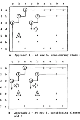
In [ 181, Hunt and Szymanski compute the ranks in a different manner. Rather than determining class 1, then class 2,..., in succession, they determine all the classes concurrently. Their algorithm works row by row and keeps track of all nonempty classes partially determined. Figure 4 provides a contrast of the ideas of Approaches 1 and 2. The vertical break lines correspond to “threshold positions;” the *‘s correspond to points that are still be to “ranked.” Other points are labelled with their ranks. Hunt and Szymanski decide the rank of a point (i + 1,j) by searching on the ordered list

O=PA <Pf<P’,<... <P;<P;+,=c.%

to find the X, such that Pf._, <j < PL (hence (i + 1,j) is in class X by Theorem 1). Since there are at most p classes, and for each point, it takes a binary search on the list of Pis, so if there are P points, at most O(lP logp) time is used for computing the “ranks,” or, equivalently, the length of LCS. When P is small, for example, P = O(n)

in some situations [ 181, ( i.e., when relatively few symbols of string A coincide with symbols of string B), their algorithm is very efficient-O(n log n), including the preprocessing.

Recently, we found that Hunt and Szymanski’s algorithm can be improved, without sacrificing the desirable features under “sparse” situations. The idea is

c b a c b a a b a la 1 2 b 1 4 d 2? 3c 1 ,9' (P$ 5 b A * ' 6 b ?? ?? ?? 7 a * ?? ?? *

a Approach 1 - at row 5, considering c b a c b a a b a 1 a 2 b 3 c 4 d 5 b 6 b 7 a ?? ? ? ?? ?? class 2

b Approach 2 - at row 5, considering classes 1, 2, and 3

FIG. 4. Two approaches at work.

simple,sinceO=Pb<P~<...<P~<P~+,= co for the partially determined classes cf ) c; )...) Ck, also, the points at row (i + 1) are kept as the ordered list PB[B, 1 ] < PB[@ 21 < a** < PB [R N[e] I, w h ere 6’=A [i + I]. So determining the ranks of the points at this row requires a “merge” of the above two ordered lists-the threshold positions and the j-values. Note that once we can determine the abovesaid merged sequence of PJs and PB,, at most O(p) time is needed for identifying the keys and the new thresholds for p classes. Hence we may concentrate on bounding the time required in doing the merge. ’

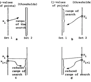
Many alternatives may determine the merged sequence as required. For example, here are some possibilities:

(1) Given an element xi from set 1 searches (with a binary search) set 2 to find the index j, so that yj < xi < yj+ , (Fig. 5(a)).

(2) Same as (l), but reverse the direction of searches (Fig. 5(b)).

’ It is pointed out to the authors that Hunt and McIlroy were the first to observe that a merge is required (see [ 171). But it is also pointed out that we went further by using efficient merging algorithms, rather than using binary searches to accomplish the merge and restricting efficiency to special cases of “sparse matches.”

THE LONGEST COMMON SUBSEQUENCE 145

'i 'i+l

IJ range of skmh d

FIG. 5. Four different schemes.

(3), (4) Same as (1) and (2), respectively, but register the result of the last

search, then avoid searching in vain (Figs. 5(c) and (d)).

Scheme (1) (or (2)) may characterize several approaches already known for solving the LCS problem, e.g., [ 17, 18, 331. For a row with n points and p classes under consideration, using scheme (1) requires O@ log n) time, and (2) requires O(n logp) time. Clearly, (3) and (4) are already improvements over (1) and (2), respectively, because of better utilization of the information obtained in the searches. It would be interesting to investigate other alternatives and analyze the effects to the performance. But now that a merge is required, we can save by using the most

efftcient merging algorithms that are already existing, e.g., [5, 19, 291, and obtain a definite improvement over any of the preceding alternatives. Note that, in the context of the LCS problem, what we require from a “merge” is actually the information regarding the relative ordering of PB[8, Xl’s and Pis obtained through the comparisons of elements of the two sets, and is not the actual output of the merged sequence. Hence, it is reasonable to consider just how many comparisons a merging algorithm requires, and neglect the “move” operations that a merging algorithm is usually supposed to do.

Therefore, with n points (j-values) to “merge” with p classes (threshold positions) at a row, at most O@ log(n/p) -t p) time, rather than O(n log p) or O@ log n) time, is

required, provided one efficient merging method such as [5, 19, 291 is adopted.2 Very

* For practical uses, simple, efficient merging methods such as a linear (tape) merge, which is already optimal for two sets with similar cardinalities [25], is suggested. For situations where sets with disparate sizes occur often, variants of binary searches (e.g., which can alternate direction of searches according to ]]Sr]] b ]]S,]] or ]]S,]] + ]]Sr]]) may be better. But for unpredictable environment, Hwang-Lin merge is recommended, as it possesses the merits of the above approaches in both the above-mentioned situations (See 1251).

roughly, for m rows, the total time needed is bounded by O(mp log(n/p) + mp). Coin- cidently, it takes almost the same form as obtained in our (deliberately devised) Algorithm 1. Note that we did not make use of intricate, special purpose data structures, such as HIGH[0], LOW[ ‘I, I w lc h’ h are indispensable to our first approach.

On the other hand, the first approach allows the possibility of parallel processing. Consider the following arrangement. Let processor 1 take care of class 1, processor 2 take care of class 2, and so on. With processor (i + 1) lags a row behind processor i and simple communications (with LOW[i] being a common variable), each processor can determine the class. So O(m log(n/m) + m) time at most is required. Incidentally, there are also parallel merging algorithms, which may speedup our second approach.

IV. DISCUSSIONS

The worst case time complexity of our Algorithm 1 is shown to be O@m log]n/m) + pm) (Theorem 2, Appendix). When n = m, this is O@n), the same as that in [ 141. When n > m, the complexity can be expressed as O@m log(n/m)). Let CI = n/m > 1, our bound is better off by a factor a/log a, which can be arbitrarily large. Interestingly, a/log (r seems to be the direct consequence of replacing a sequential search by a binary search. But we are not able to predict when another search scheme is used.

Our algorithm also exhibits a desirable property which is now explained. By our analysis (Theorem2, Appendix), the time complexity of our algorithm can also be expressed as O(lK log@n/lK) f IK), or, more loosely, O(IK log n), where IK being the number of all keys (the minimal K-candidates, as defined in [ 141). Hence if the number of matches is rather few (“sparse” matches) our algorithm is very efficient. It even outperforms the O(lP log n) algorithm in the same sparse situations, since IK < P

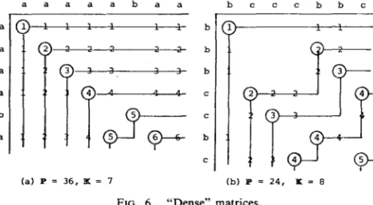
(total number of matches). Furthermore, even in some very “dense” situation (which is not uncommon, if two objects represented by the strings are very much similar), such as in Fig. 6, our algorithm is still very efficient, as the running time is deter- mined by the number of keys (IK) which does not increase the same way as P does.

a a a a a b a a (a) P = 36, K = 7 bcccbbc 1 3 2 4

i-it3

THE LONGEST COMMON SUBSEQUENCE 147

Recall that in our algorithm, the binary searches are initiated only when a key is encountered; otherwise, only very simple bookkeeping operations are performed. But the O(lP log n) algorithm requires a binary search for every point, hence it may become one that requires as much as O(mn log rz) time.

Up to the present, the best asymptotic upper bound is due to Masek and Paterson, in [30]. The approach is basically that of Arlazarov et al. [4], usually known as the Four Russians, in computing transitive closures of Boolean matrices. They proved that if an n X n matrix was split up into submatrices of a certain size and computations on all possible submatrices of this size were first performed, the problem could be solved using 0(n3/log n) operations, instead of 0(n3) operations of the simple common approach. Likewise, Masek and Paterson’s algorithm works by splitting up the computation of the “L matrix”, mentioned in the dynamic programming approach, into many smaller computations, then putting them together to get the final result. The time complexity of this algorithm is O(n . max(1, m/log n)) compared with ours of O@m - max(1, log(n/m))) (Corollary 2.1, Appendix). Our

algorithm may be comparable when p is relatively small. It should be cautioned that their time complexity is based on the logarithmic cost criterion, rather than on the usual uniform cost criterion. Also, the above bound applies only asymptotically- when the lengths of the strings are a great many times the size of the alphabet. Hence, the performance of an actual implementation of this method cannot beat that of the previously mentioned approaches in the usual situations. Because the overhead of precomputing all the submatrices often will not be compensated in the later “referencing” phase. Nonetheless, the approach per se is interesting enough, besides, the bound is the best.

Aho et al. [ 1, 21 investiagted the lower bound achievable for a class of LCS algorithms. They showed that, under a slightly restricted model of computation, where the “equal-not-equal” comparisons (is a = b?) of two symbols were the only information sources, every algorithm takes at least O(mn) operations to solve the LCS problem. In this sense, Wagner and Fischer’s algorithm [40] is already optimal. Hence, we can do no better than O(nm) without using extra information. Wong and Chandra in [42] derived a similar lower bound for the string editing problem, which is also applicable to the LCS problem. But their model of computation is also restricted, hence the bound need not apply to all algorithms.

For many conceivable applications, it is reasonable to assume a linear ordering on the symbol set. This provides extra information, as it makes useful operations such as test-for-greater comparisons (is a > b?) possible. Recall that the string identification problem, mentioned in Section II, can be solved in O(n log n) time rather than in O(n”), when an ordering of symbols is assumed, n being the length of the string. When the symbol set is further assumed to be known beforehand, then only O(n) time is required. Now, for the LCS problem, with the symbol set given, the best algorithm requires O(nm/log n), but the best lower bound for the algorithms under this assumption is O(n) [42]; some investigation in filling the gap still seems profitable [301.

Our measure of “efficiency” of an algorithm was necessarily in terms of worst case

(rather than average case) time complexity (rather than space complexity). The reason for this lack of generality is due to the absence of “average case” literature, and to the fact that “time” is the relatively more valuable resource. Indeed, to define a meaningful probability distribution for the inputs is considered a difficult problem

[2]. Specific applications may justify further studies.

APPENDIX

Now we analyze the worst-case time complexity of Algorithm 1: The loop from Step 2 to Step 6 is executed p + 1 times, p being the number of nontrivial classes. Step 2 takes O(m) per execution. The total time is therefore bounded by O@m). Steps 3-5 take constant time per execution, hence bounded by O(p).

Step 6.1 takes O@m) totally; the test in Step 6.2 takes similar amounts of time. Step 6.3 is executed at most pm times (totally), thus bounded by O@m). It takes similar amounts of time to decide which one of the three cases in Step 6.4 is to be executed.

When Case 1 is encountered, only constant time is consumed, and therefore O@m) time at most in total. Similarly, the total time for Case 2 is O@m). Case 3 needs some careful treatment.

Let X, be the range (upon which a binary search is initiated) when Case 3 is encountered the eth time, and qk be the total number of occurrences of Case 3 when considering C,. As our discussion following Algorithm Al reveals, the ranges of separate binary searches are nonoverlapping, hence

x, +x* +

where n is the number of all j-values and s is the number of all distinct symbols in string A (N[B] = 0 if 8 does not appear in B).

Note that a binary search is done if and only if a key is present, so

q/c

= II

KEYWI

Now, the time complexity of a binary search can be measured by the number of comparisons done in the worst case. Let W, denote the total number of comparisons devoted to the binary searches when considering C,, then3

w, < ]log(x, + I)] + [log(x, + l)] + **a + ]log(.$ + l)] = [log Xi] + 1 + llog X2J + I + ’ ** + llog x4J + 1 ~(logx,+logx,+~~~+logX4~)+qk.

THE LONGEST COMMON SUBSEQUENCE 149

By simple application of Lagrange multiplier method [43], it can be shown that (log xi + log x2 + * ’ * + log x,J achieves a maximum when all x/s are equal. By setting Xi = n/q,, we have,

W&log;+&. Thus, in the worst case, for p classes

w=

w,=

2

I<k<o l<k<o

Letting CIGkGp qk = IK (total number of keys),

W<IKlogn+IK- c qklogqk.

l<k<p

Again, the Lagrange multiplier method can be used to show that xlGkGp qk log qk is minimum when all qi)s are equal, i.e., qk = IK/p, for all k, therefore

W<lKlogn+IK-+log;

= IK log E + IK.

_PI

Thus, in terms of the number of keys (IK) and the length of LCS @), we may bound all the work done in Case 3 by O(IK log@n/lK) + IK), or O(IK log n), since p < m < n. In order to measure the work in terms of only p, m, and n, we reconsider the relation in (A)

wk6?k10g;+qk.

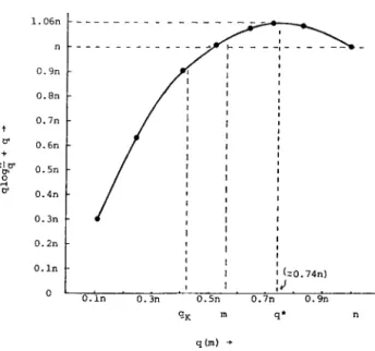
The right-hand side (qk log(n/q,) + qk) monotonically increases as qk goes from 1 to n . exp(ln 2 - l)-let q* denote this value-then it decreases again as qk goes from q* to n.

Note that qk, the number of keys in a class, cannot exceed m, as each row contains at most one key for any class (cf. Fig. 2), i.e., qk < m < n. Figure 7 depicts the curve for q log(n/q) + q versus q. From the figure we see that

(1) when m < n . exp(ln 2 - I),

(2) when naexp(ln2- l)<m<n,

0.9n 0.h - 0.7n - I I I 0.2n - t I I I 0 1 I 0.h - I I I I I 1 k0.74n) I I o- ' .IJ. . 0.h 0.3ll 0.5n 0.7n 0.9n qK m q* l-8 qlm) *

FIG. 7. q log(n/q) + q VerSuS 9.

Combining (C) and (D), we have

and for p classes,

w=o

c pmlog~+pm . 1

THEOREM 2. The worst-case time complexity of Algorithm 1 may be expressed as

O(lK log(n/lK) + IK) or O@m log(n/m) + pm). The storage space required can be bounded by O(IK), or O@m), if linked list structure is adopted for keeping KEY(K).

COROLLARY 2.1. The time complexity of Algorithm Al can be expressed as

O@m . max( 1, log(n/m)) or O(m’ . max( 1, log(n/m)).

ACKNOWLEDMENTS

The referees (anonymous) pointed out several flaws in our previous expositions and indicated possible enhancements, which helped us greatly. We are indebted to them.

THE LONGEST COMMON SUBSEQUENCE 151

REFERENCES

1. A. V. AHO, D. S. HIRSCHBERG, AND J. D. ULLMAN, Bounds on the complexity of the maximal common subsequence problem, in “Proceedings, 15th Ann. IEEE Sympos. on Switching and Automata Theory, 1974,” pp. 104-109.

2. A. V. AHO, D. S. HIRSCHBERG, AND J. D. ULLMAN, Bounds on the complexity of the longest common subsequence problem, J. Assoc. Comput. Much. 23 (1) (1976), 1-12.

3. A. V. AHO, J. E. HOPCROFT, AND J. D. ULLMAN, “The Design and Analysis of Computer Algorithms,” 2nd ed., Addison-Wesley, Reading, Mass. 1976.

4. V. L. ARLAZAROV, E. A. DINIC, M. A. KRONROD, AND I. A. FARADZEV, On economic construction of the transitive closure of a directed graph, Dokl. Akad. Nauk SSSR 194 (1970), 487-488 [Russian]; Soviet Math. Dokl. I1 (5) (1970), 1209-1210.

5. M. R. BROWN AND R. E. TARJAN, A fast merging algorithm, .Z. Assoc. Comput. Much. 26 (2) (1979), 21 l-266.

6. V. CHVATAL, D. A. KLARNER, AND D. E. KNUTH, Selected combinatorial research problems, Technical Report No. STAN-CS-72-292, p. 26, Stanford Univ., Stanford, Calif., 1972.

7. V. CHVATAL AND D. SANKOFF, Longest common subsequences of two random sequences, Technical Report No. STAN-CS-75-477, Stanford Univ., Stanford, Calif., Jan. 1975.

8. M. 0. DAYHOFF, Computer aids to protein sequence determination, .Z. Theoret. Biol. 8 (1965) 97-l 12.

9. M. 0. DAYHOFF, Computer analysis of protein evolution, Sci. Amer. 221 (1) (1969), 86-95.

10. M. L. FREDMAN, On computing length of the longest increasing subsequences, Discrete Math. 11 (1) (1975), 29-36.

11. K. S. Fu AND B. K. BHARGAVA, Tree systems for syntactic pattern recognition, IEEE Trans.

Comput. C-22 (12) (1973) 1087-1099.

12. J. GALLANT, D. MAIER, AND J. A. STORER, On finding minimal length superstrings, J. Comput.

Sysrem Sci. 20 (1980), 50-58.

13. D. S. HIRSCHBERG, A linear space algorithm for computing maximal common subsequences, Comm. ACM 18 (6) (1975) 341-343.

14. D. S. HIRSCHBERG, Algorithms for the longest common subsequence problem, .Z. Assoc. Comput.

Mach. 24 (4) (1977), 664-675.

15. D. S. HIRSCHBERG, “The Longest Common Subsequence Problem,” Ph.D. thesis, Princeton Univ. Princeton, N. J., 1975.

16. W. J. Hsu AND M. W. Du, “A Fast Algorithm for the Longest Common Subsequence Problem,” Yearly Report for NSC support, March 1982.

17. J. W. HUNT AND M. D. MCILROY, “An Algorithm for Differential File Comparison,” Computing Science Technical Report No. 41, 197.

18. J. W. HUNT AND T. G. SZYMANSKI, A fast algorithm for computing longest common subsequences,

Comm. ACM 20 (5) (1977), 35&353.

19. F. K. HWANG AND S. LIN, A simple algorithm for merging two disjoint linearly ordered sets, SIAM

J. Comput. 1 (1972), 31-39.

20. S. T. ITOGA, The string merging problem, BIT 21 (1981), 20-30.

21. B. W. KERNIGHAN AND L. L. CHERRY, A system for typesetting mathematics, Comm. ACM 18 (3) (1975), 151-157.

22. D. E. KNUTH, Big omicron and big omega and big theta, SZGACT News, 8 (2) (1976), 18-24. 23. D. E. KNUTH, J. H. MORRIS, AND V. R. Pa~rr, “Fast Pattern Matching Algorithms,” Technical

Report No. STAN-CS-74440, Computer Science Dept., Stanford Univ., Stanford, Calif., 1974. 24. D. E. KNUTH, “The Art of Computer Programming, Vol. 1: Fundamental Algorithms,” Addison-

Wesley, Reading, Mass., 2nd ed., 1973.

25. D. E. KNUTH, “The Art of Computer Programming, Vol. 3: Sorting and Searching,” Addison- Wesley, Reading, Mass., 1973.

26. R. LOWRANCE AND R. A. WAGNER, An extension of the string to string correction problem, .I.

Assoc. Comput. Mach. 22 (2) (1975), 177-183.

27. S. Y. Lu AND K. S. Fu, A sentence-to-sentence clustering procedure for pattern analysis, IEEE Trans. Systems Man Cybernet. SMC-8 (5) (1978), 381-389.

28. D. MAIER, The complexity of some problems on subsequences and supersequences, J. Assoc. Comput. Mach. 25 (2) (1978), 322-336.

29. G. K. MANACHER, Significant improvements to the Hwang-Lin merging algorithm, J. Assoc. Comput. Mach. 26 (3) (1979), 434440.

30. W. J. MASEK AND M. S. PATERSON, A faster algorithm computing string edit distances, J. Comput. System Sci. 20 (1980), 18-3 1.

31. H. L. MORGAN, Spelling correction in systems programs, Comm. ACM 13 (2) (1970) 90-94. 32. J. H. MORRIS AND V. R. PRATT, “A Linear Pattern-Matching Algorithm,” Technical Report No.

TR-40, Comput. Center, U. of California, Berkeley, Calif., 1970.

33. A. MUKHOPADHYAY, A fast algorithm for the longest-common-subsequence problem, Inform Sci. 20 (1980), 69-82.

34. S. B. NEEDLEMAN AND C. S. WUNSCH, A general method applicable to the search for similarities in the amino acid sequence of two proteins, .I. Molecular Biol. 48 (1970) 443-453.

35. D. SANKOFF, Matching sequences under deletion insertion constraints, Prbc. Nut. Acad. Sci. U.S.A.

69 (1972), 4-6.

36. D. SANKOFF AND R. J. CEDERGREN, A test for nucleotide sequence homology, J. Molecular Biol. 77 (1973), 159-164.

37. S. M. SELKOW, The tree-to-tree editing problem, Inform. Process. Len. 6 (6) (1977) 184-186. 38. P. H. SELLERS, An algorithm for the distance between two finite sequences, J. Combin. Theory Ser.

A 16 (1974), 253-258.

39. R. A. WAGNER, Common phrases and minimum-space text storage, Comm. ACM 16 (3) (1973) 148-152.

40. R. A. WAGNER AND M. J. FISCHER, The string-to-string correction problem, J. Assoc. Comput. Mach. 21 (1) (1974), 168-173.

41. P. A. WAGNER, On the complexity of the extended string-to-string correction problem, in

Proceedings, 7th Ann. ACM Sympos. on Theory of Comput. 1975, pp. 218-223.

42. C. K. WONG AND A. K. CHANDRA, Bounds for the string editing problem, J. Assoc. Comput. Mach. 28 (1) (1976), 13-18.

43. F. S. HILLIER AND G. J. LIEBERMAN, “Introduction to Operations Research,” Holden-Day, San Francisco.