Applying the seasonal error correction model to the
demand for international reserves in Taiwan
Tai-Hsin Huanga, Chung-Hua Shenb,U
a
Department of Economics, TamKang Uni¨ersity, Tamsui, Taiwan
b
Department of Money and Banking, National Chengchi Uni¨ersity, Mucha, Taipei 116, Taiwan
Abstract
A dynamic demand function for international reserves based on the seasonal difference is derived. Our model of using seasonal difference distinguishes the present study from previous studies in three aspects. First, the dependent variable is seasonally differenced instead of being first order differenced. Next, the local money market disequilibrium included is also in fourth difference form. Finally, given the existence of stochastic seasonal-ity, a new model, using a seasonal error correction rather than the conventional error correction, is specified and estimated. Based on this new specification, the results yielded
are more sensible than those of using a differenced model. 䊚 1999 Elsevier Science Ltd.
All rights reserved.
JEL classifications: F30; F32; C22
Keywords: International reserve; Seasonal unit root; Seasonal cointegration
1. Introduction
Studies of the demand for international reserves are typically based on one of two theories. The demand-for-reserve theory asserts that reserves are held to finance international transactions and to serve as a buffer stock to meet unex-pected payment difficulties. This theory asserts that reserve holdings change in
UCorresponding author. Tel.:
q886 2 9393091 81020; fax: q886 2 9398004; e-mail: chshen@nccu.edu.tw 0261-5606r99r$ - see front matter 䊚 1999 Elsevier Science Ltd. All rights reserved.
Ž .
response to the discrepancy between desired reserves and actual reserves, where the desired demand function for reserves depends on three key variables: a measure of the variability in the balance of payments, the scale of the country, and
Ž
the average propensity to import see Kenen and Yudin, 1965; Clower and Lipsey, .
1968; Heller and Khan, 1978; Frenkel, 1983; Elbadawi, 1990 . Once the key determinants are determined, the empirical tests typically rely on a partial
adjust-Ž .
ment mechanism PAM to replace the unobserved desired reserve by its actual counterpart. The adjustment speed and the dynamic process can be inferred from the coefficient on the lagged dependent variable.
Another explanation of the behavior of holding reserves is provided by a simple version of the monetary approach to the balance of payments. This approach focuses on the asset side of the balance sheets of financial institutions, where the money supply is equivalent to the sum of foreign assets and domestic credit. Hence, for given domestic credit, changes in international reserves will be related to changes in the demand for money. The level of international reserves are
Ž . Ž .
expected to rise fall if there is an excess demand supply for money. Internatio-nal reserves are therefore viewed as a residual according to the monetary ap-proach.
A synthesis of the demand for reserves theory and the monetary approach, as
Ž .
claimed by Edwards 1984 , can be obtained if there is a stable demand for international reserves. As long as a stable demand for reserve exists, domestic credit cannot be exogenous. Money market disequilibria will also affect reserve
Ž .
holdings. To integrate these two different explanations explicitly, Edwards 1984 incorporates an additional variable, excess money demand, representing an extra adjustment cost between the actual and the desired reserves in the PAM. His underlying assumption is that reserve holdings can be affected by money-market disequilibria only in the short-run, arising possibly from a domestic economic disequilibrium. The resulting reduced form of the demand for reserves equation includes not only the three key determinants, but also the money market disequi-librium.
Though the monetary approach stresses that money-market disequilibria have a
Ž .
significant short-run positive effect on the demand for reserve, Elbadawi 1990 pursued this further by examining whether or not money-market disequilibria influence reserves in the long-run specification. He applied the recent econometric
Ž .
technique of cointegration, together with the error correction mechanism ECM to investigate both the short-run dynamics and the long-run equilibrium
relation-Ž .
ships. Ford and Huang 1994 also employed the ECM to specify the relationship
Ž .
between reserves and their determinants. In contrast to Elbadawi 1990 , their money-market disequilibrium appeared only in the short-run dynamic process.
Ž . Ž .
Although Elbadawi 1990 and Ford and Huang 1994 successfully improved the demand function for reserves by explicit consideration of the dynamic process, their models cannot be easily generalized to other countries. The theoretical
Ž . Ž .
optimizing a conventional partial-adjustment type loss function involving two sources of adjustment costs: the gap between desired and actual levels of reserves and the first difference between current and lagged reserves. However, in many developing countries, the data are typically not seasonally adjusted. The official annual growth rate of economic data is typically computed as a log difference over the latest 12-month period, generally referred to as a seasonal difference. Hence, the adjustment costs of reserves in developing countries are better modeled by seasonal differences than first differences. This minor correction, however, causes the subsequent regression specification to be modified substantially. It follows that, the loss functions for these developing countries should incorporate these specifi-cation changes.
Ž . Ž .
Furthermore, the models of Elbadawi 1990 and Ford and Huang 1994 are subject to an estimation bias. Prior to their use of the ECM, they adopt the
Ž .
two-step approach of Engle and Granger 1987 to examine whether or not
Ž .
reserves and their determinants are cointegrated. Gonzalo 1994 demonstrated that the Engle and Granger two-step cointegration procedure yields weak and biased results when the model has more than two series. As an alternative, the
Ž .
maximum likelihood approach of Johansen 1988 and Johansen and Juselius
Ž1990 can be utilized, which takes advantages of its robustness in a multivariate.
Ž .
setting see Gonzalo, 1994; Hargreaves, 1994 .
Ž . Ž .
This paper generalizes the Elbadawi 1990 and Ford and Huang 1994 demand function for reserves for those countries lacking seasonally adjusted data. The loss function is specified within the framework of seasonal differences, which for quarterly data can be expressed as four seasonal unit roots. The existence of a seasonal difference may cause the conventional cointegration tests, e.g. the two-step
Ž .
procedure of Engle and Granger 1987 and the maximum likelihood method of
Ž . 1
Johansen 1988 , to be inappropriate at the zero frequency. A more appropriate
Ž .
approach is to employ the Lee 1992 maximum likelihood approach to examine the seasonal cointegration relationships among variables. The following seasonal
Ž .
error correction mechanism SECM , not only correctly integrates the reserve-demand theory with the monetary approach for a country lacking seasonally adjusted data, but also explicitly specifies the entire short-run dynamics and long-run equilibrium of the reserves. Hence, previous approaches, using either PAM or ECM become special cases of our approach.
To exemplify our approach, we select the demand for reserves in Taiwan as an example. Taiwan is chosen due to its unique position of holding a large stock of international reserves, the third largest globally. Also, the data of Taiwan are typically not seasonally adjusted and its official growth rate is calculated by means
1
Ž .
Engle et al. 1989 show that the conventional cointegration estimate is inconsistent if unit roots of distinct seasonal frequencies are regressed. Moreover, the long-run relationships among seasonal frequencies are also neglected in the conventional cointegration test.
Ž . Ž . of a seasonal difference. Similar to Elbadawi 1990 and Ford and Huang 1994 , the same key determinants and money market disequilibria are selected in the desired demand equation for reserves. However, the loss function differs from the above authors in that it utilizes a seasonally differenced form, thus conforming with Taiwan’s official growth rate. Although Taiwan’s data are used as an example, the generalization to other countries lacking seasonally adjusted data is immediate.
Our results are fruitful. First, we demonstrate that our general specification is preferable to the conventional Johansen’s modelling in three aspects. The new
Ž 2.
model yields a better goodness of fit higher adjusted R , a stable functional form
Žpassing both Chow and the normality tests , and an expected positive structural.
coefficient on income. By contrast, the conventional specification has a poorer model fit, fails to pass the stability test, and yields a wrong negative structural coefficient on income. Accordingly, those countries without seasonally adjusted data are encouraged to use our approach to account for movements in their reserves. Furthermore, even countries with seasonally adjusted data could benefit from our model. This is because the stochastic seasonality in the raw data cannot be fully removed by either including seasonal dummies or by utilization of the
2
Ž . Ž .
official X-11 method. For example, Ghysels et al. 1993 ; Ghysels 1994 and
Ž .
Ericsson et al. 1994 have suggested that X-11 adjusted data not be used to fit models. The ideal procedure, suggested by them, is to use seasonal cointegration and apply the resulting SECM to investigate the demand for reserves.
In addition to the above results, we find that while a high speed of adjustment towards equilibrium for the reserve holdings is found in previous literature, a markedly low speed of adjustment is discovered here. According to the theory of
Ž .
Clark 1970b , such a low adjustment speed is probably due to the huge stock of reserve holdings by a country. This is consistent with Taiwan’s situation. Because Taiwan is currently not an IMF member, has a precarious political entanglement with mainland China, and has few official diplomatic relations with other countries, it needs to hold a significant amount of reserves in case of emergency. The low adjustment rate reflects the reluctance of the authority in Taiwan to adjust actual reserves to the economically desired level.
Finally, using our generalized approach, we find that a long-run equilibrium relationship exists at the zero frequency among the reserves, their determinants, and money. The monetary approach as well as the demand-for-reserve theory are also found to jointly account for the long- and short-run movements of Taiwan’s
Ž .
reserves. We also find that the narrow money market M1B is a more appropriate monetary aggregate for disequilibrium as a determinant to the demand for reserves
Ž .
than is broad money M2 .
2
Ž .
The study of Abeysinghe 1991 demonstrates that inclusion of seasonal dummies cannot eliminate the Ž .
stochastic seasonality embedded in most macroeconomic time series. Also, Wallis 1974 , Ghysels et al. Ž1993 , Ghysels 1994 , and Ericsson et al. 1994 do not suggest applying the method of X-11 to adjust. Ž . Ž . raw data.
The remainder of this paper is organized as follows. Section 2 derives a function for the demand for reserves, which will be estimated using Taiwanese data, by minimizing a loss function commonly used in the literature. Section 3 briefly discusses the testing procedures for seasonal unit roots and seasonal cointegration. Section 4 presents and analyzes the empirical results. Our findings are finally summarized in Section 5.
2. The theoretical model
Ž .
The long-run demand for reserves at time t is similar to that of Elbadawi 1990
Ž U . Ž U
with the money market disequilibrium mt y mty1 being replaced by mt y
.
mty4 .
U Ž U . Ž .
rt s a q a y q a0 1 t 2 q a im q a m y mt 3 t 4 t ty4 1
where rU denotes the desired stock of real international reserves, y denotes the
real GNP, denotes a measure of the variability in the balance of payments, im
Ž
denotes the average propensity to import being the ratio of real imports to real
. U
GNP , and m and m are the desired and actual stocks of money held,
respec-tively. All variables, except for the interest rate, are in the log form.
Our proxy for the scale variable, y, is expected to have a positive effect on the
Ž .
demand for reserves see Heller and Khan, 1978; Frenkel, 1983; Elbadawi, 1990 ,
and its coefficient, a , is thus positive. Reserves are expected to be positively1
influenced by variability to accommodate fluctuations in the foreign trade factor
Žsee Kenen and Yudin, 1965; Clower and Lipsey, 1968 ; thus, a should also be. 2
positive. The impact of im on the demand for reserves, however, is uncertain. On
Ž .
the one hand, Frenkel 1974 has stressed that reserves are positively associated with the degree of openness, which can be proxied by im. On the other hand,
Ž . Ž . Ž .
Heller 1966 , Grubel 1969 and McKinnon and Oates 1966 , have derived an inverse relation between im and reserve holdings via output adjustments in a
Keynesian model. The sign of a is therefore theoretically indeterminant.3
Ž U .
The monetary disequilibrium mt y mty4 is used in accordance with the partial
adjustment model below. According to the monetary approach to the balance of
Ž U .3
payments, mt y mty4 , which represents the effect of money market
disequilib-rium, is anticipated to have a short-run positive effect. In contrast, the traditional demand for reserves theory excludes the role of monetary disequilibrium. It postulates that discrepancies between the desired and the actually held stock of reserves are the main sources of movements in reserves. According to Edwards
Ž1984 , the contradiction between the monetary approach and the demand for.
reserves theory can be reconciled by allowing the sign of a to be negative.4
3
Ž . Ž . Ž .
Edwards 1984 , Elbadawi 1990 , and Ford and Huang 1994 , among others, postulated that the effect
Ž U .
The one period loss function employing a seasonally differenced annual growth
rate is thus:4
Ž U. Ž . Ž U U . Ž . Ž .
Ls d r y r q d r y r1 t t 2 t ty4 y 2 d r y r3 t ty4 rty rty4 2
where d is the cost of deviation from long-run equilibrium and d is the short-run1 2
Ž .
transaction cost. The cross-product term in Eq. 2 states that the adjustment cost can be reduced, if the desired and actual reserve holdings move in the same
Ž .
direction. The three coefficients are all positive. Hendry and Sternberg 1981 Ž . demonstrated that an EC model can be obtained by minimizing Eq. 2 with
respect to r . Taking the first derivative with respect to r and rearranging termst t
yields
Ž U . Ž U U . Ž .
⌬ r s r y r4 t t ty4s r1 ty4y rty4 q r y r2 t ty4 3
Ž . Ž . Ž .
where s d r d q d and s d q d r d q d . It is interesting to note1 1 1 2 2 1 3 1 2
U Ž .
that the first term rty4y rty4 is simply the conventional error correction EC
term lagged four periods. Hence, is referred to as the speed of adjustment or1
Ž .
‘loading’ of the disequilibrium of demand for reserves. Substituting Eq. 1 into Eq.
Ž .3 yields w x Ž U . ⌬ r s4 t a q a y1 0 1 ty4q a2ty4q a im3 ty4y rty4 q a m1 4 ty4y mty8 U 2Ž . Ž . q a ⌬ y q a ⌬ q a ⌬ im q a ⌬ m y m2 1 4 t 2 4 t 3 4 t 4 4 t ty4 4
This equation, which is derived from a one-period loss function, coincides with the
Ž .
seasonal error correction model as explained shortly . It will be seen later that diagnostic checks and cointegration tests of this model are also different from
Ž . previous works, e.g. Eq. 6 .
Ž .
Estimating Eq. 4 requires all variables to be stationary. The first bracket term Ž .
on the right hand side of Eq. 4 is stationary if variables y, , im, and r all have
Ž U
unit roots at the zero frequency and are cointegrated. The second term mty4y
. Ž . U
mty8 in Eq. 4 represents the disequilibrium in the money market. Since mt is
Ž U U .
unobservable, mt y mty8 is typically replaced by its linear projection, ⌬ m ,4
ˆ
twhich should ordinarily be a stationary process. The third term on the right hand side of the equation is also stationary because each component in the term is in its seasonally differenced form.
Ž .
Eq. 4 is referred to as a ‘structural’ form equation here, whereas its reduced
4
Ž .
This model is a direct extension of the model of Hendry and Sternberg 1981 , which uses the first
Ž U. Ž . ŽU U .Ž .
form equation can be written as
⌬ r s b q b EC q b ⌬ m
ˆ
q b ⌬ y q b ⌬ q b ⌬ im q b ⌬2mˆ
4 t 0 1 ty4 2 4 ty4 3 4 t 4 4 t 5 4 t 6 4 t
Ž .5
where each reduced form coefficient matches its corresponding combination of Ž .
structural form coefficients in Eq. 4 . Since the matchings are natural, their expressions are suppressed here.
Following similar derivations, the conventional cointegration specification can be expressed as:
2 Ž .
⌬r s c q c ECt 0 1 ty1q bc ⌬m2
ˆ
ty1q c ⌬ y q c ⌬3 t 4 q c ⌬im q c ⌬ mt 5 t 6ˆ
t 6Ž . Ž .
Eqs. 5 and 6 will be referred to as the seasonal cointegration specification and conventional cointegration specification, respectively. The performances of these two different specifications are of primary concern to us.
Ž .
The empirical testing procedure of Eq. 5 includes the following four steps.
First, ⌬ m and ⌬2m are estimated. This can be achieved by applying Lee
ˆ
ˆ
4 ty4 4 t
Ž1992 seasonal cointegration approach to find appropriate variables that are.
seasonally cointegrated with the money stock. The subsequent linear projectors of
2 Ž .
⌬ m4
ˆ
ty4 and ⌬ m act as new proxy variables to be used in Eq. 5 . Next, the4ˆ
testimated ECty4 can be obtained by using a cointegration approach again to find
the equilibrium relationships among y ,t , im and r at the zero frequency. Thet t t
Ž .
subsequent equilibrium error at the zero frequency is the term ECty4 in Eq. 5
lagged four periods. Third, the same four variables should be tested to determine if
they are seasonally cointegrated at the 1r2 and 1r4 frequencies. If the
cointegrat-ing relationships are found at those frequencies, their equilibrium errors ᎏ
Ž . Ž .
seasonal error correction terms ᎏ must be included in Eq. 5 . Eq. 5 can now be
Ž . Ž .
called a seasonal error correction model SECM . Finally, Eq. 5 is estimated by OLS.
3. Seasonal integration and cointegration
Ž . Ž .
Hylleberg et al. 1990 and Engle et al. 1992 have derived seasonal unit root and cointegration tests. Their testing procedures are a direct generalization of the
Engle᎐Granger two-step procedure to the test for seasonal cointegration and,
Ž . Ž .
hence, suffer the same difficulties discussed in Gonzalo 1994 . Lee 1992 general-izes the maximum likelihood estimation and inference proposed by Johansen to the
Ž .
tests for seasonal cointegration for a non-stationary vector autoregressive VAR Ž
system. Under the assumptions of no deterministic components e.g. a constant, .
linear andror quadratic trends, and seasonal dummies , Lee presents asymptotic as
well as finite sample quantile distributions obtained by Monte Carlo simulations. As the critical values on the seasonal cointegration tests provided by Lee have
dimensions only up to three and are generated under the suppositions that the statistical models do not contain deterministic components, the critical values have limited use. Since the statistical models considered herein have more than three non-stationary variables and include various forms of deterministic components, our own critical values are generated by Monte Carlo simulations.
The preceding section requires the testing of seasonal cointegration. However, prior to this testing procedure, a seasonal unit root test must be first performed.
3.1. HEGY testing for seasonal unit roots
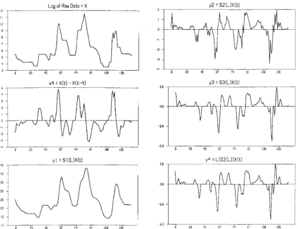
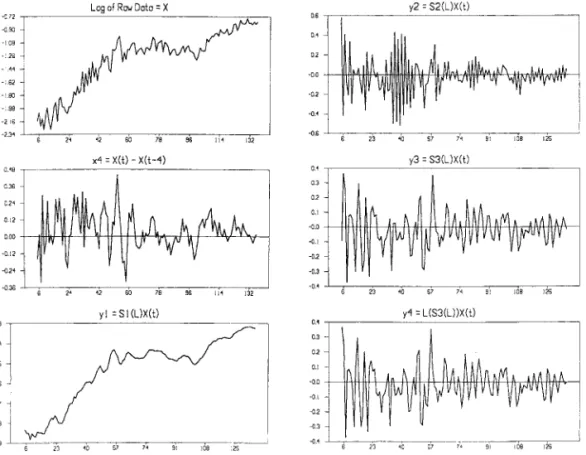
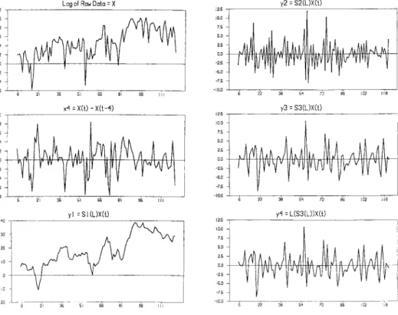
For a seasonally unadjusted series, HEGY introduces a factorization of the seasonal differencing polynomial for quarterly data as follows:
Ž 4. Ž . Ž . Ž 2. Ž .
⌬ x s 1 y L x s 1 y L 1 q L 1 q L x4 t t t 7
where x contains four unit roots,t q1, y1, i, and yi, that correspond to zero
Ž . Ž .
frequency s 0 , 1r2 cycle per quarter s 1r2 or two cycles per year, 1r4
Ž .
cycle and 3r4 cycle per quarter s 1r4 or one cycle per year. The procedure to
test these roots involves estimating the regression
Ž . Ž .
L ⌬ x s y4 t 1 1 ty1q y2 2 ty1q y3 3 ty1q y4 3 ty2q⑀t 8
Ž . Ž .Ž 2. Ž . Ž .Ž 2.
where y1 ts S L x s 1 q L 1 q L x , y s S L x s y 1 y L 1 q L x1 t t 2 t 2 t t
Ž . Ž 2. Ž .
and y3 ts S L x s y 1 q L x . S L is a seasonal filter that removes unit3 t t 1
Ž . Ž . Ž .
roots at all seasonal frequencies i.e. s 1r2 and 1r4 , whereas S L and S L2 3
eliminate unit roots at seasonal frequencies s 1r2 and s 1r4, respectively,
Ž .
as well as at the zero frequency. In estimating Eq. 8 , the unit root found at zero
frequency in x implies accepting the null thatt is zero. Similarly, a finding1
s 0 implies a seasonal unit root y1. If both and are zero, a seasonal2 3 4
unit root"i exists. Hence, rejection of both a test for and a joint test for 2 3
and implies the absence of seasonal unit roots. HEGY proposed t-statistics for4
s 0 and s 0 and an F-statistic for s s 0, which are denoted t , t1 2 3 4 1 2
Ž .
and F , respectively. Ghysels et al. 1994 propose F-statistics to test34 s s2 3
s 0 and s s s s 0, which are denoted as F4 1 2 3 4 234 and F1234,
respec-tively.
3.2. Lee’s seasonal cointegration
The testing procedure of seasonal cointegration based on the contribution of
Ž .
Lee 1992 is briefly introduced below. We assume that ⑀ are i.i.d. n-dimensionalt
Gaussian random vectors with zero mean and a variance᎐covariance matrix ⍀,
Ž .
wheras X is an n-dimensional vector with components x , x , . . . , xt 1 t 2 t n t , and p is
⌬ X s ⌸ Y4 t 1 1 ty1q ⌸ Y2 2 ty1q ⌸ Y3 3 ty1q ⌸ Y4 4 ty1q A ⌬ X1 4 ty1
Ž .
q ⭈⭈⭈ qA ⌬ X1 4 typq4q⑀t 9
Ž .
which is similar to the seasonal unit root test of Eq. 8 except that the lower case x and y denote univariate processes, whereas the capital letter X and Y denote
Ž . Ž .
multivariate processes. Namely, Y1 t and Y2 t are equal to S L X and S L X ,1 t 2 t
Ž 2.
respectively. For notational convenience, Lee redefined Y3 ty1 as L 1y L X andt
Ž 2. 5
Y4 ty1 as 1y L X . As the coefficient matrices ⌸ , . . . , ⌸ convey informationt 1 4
concerning the long-run behavior of the series, their properties must be
investi-gated in detail. If the matrix ⌸ has full rank, all series considered are stationaryk
at the corresponding frequency. If the rank of ⌸ is zero, seasonal cointegration atk
that frequency does not exist among the variables. For the intermediate case in
Ž .
which 0- rank ⌸ s r - n, a linear combination of non-stationary variables isk
stationary at the corresponding frequency.
Lee recommended four tests concerning the rank of ⌸ to implement tests ofk
seasonal cointegration. Namely, a cointegration test at frequency s 0, s 1r2,
s 1r4 and the joint test of s 1r4 and s 3r4. Since the last two tests are
asymptotically equivalent, only the test of s 1r4 is implemented here.6
4. Empirical results
4.1. Results of the test for seasonal unit roots
Quarterly data covering the period from 1961:1 to 1995:2 are used. Two measures of money aggregates, M1B and M2, are alternatively employed. Interna-tional reserves r are defined as the foreign assets of the central bank of Taiwan. The proxy scale variable y is taken to be real GNP and the exchange rate ex is
Ž .
represented by the amount of New Taiwan NT per US$ dollar. The consumer price index cpi is used to transform nominal variables into real terms. The interest rate r1 is proxied by the 1-month time deposit rate of the first commercial bank since a consistent series for money market rates was not available until 1981. The
Ž .
definition of variability in the balance of payments is the same as Elbadawi
Ž1990 and Ford and Huang 1994 and, therefore, is not defined here. With the. Ž .
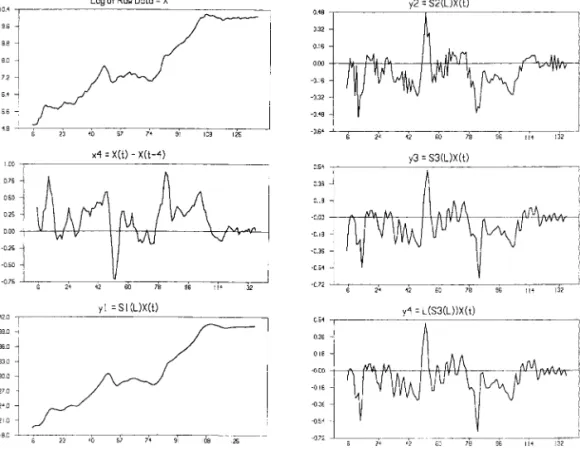
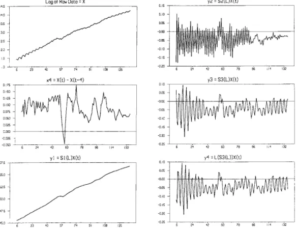
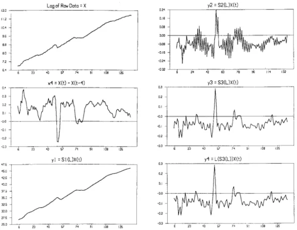
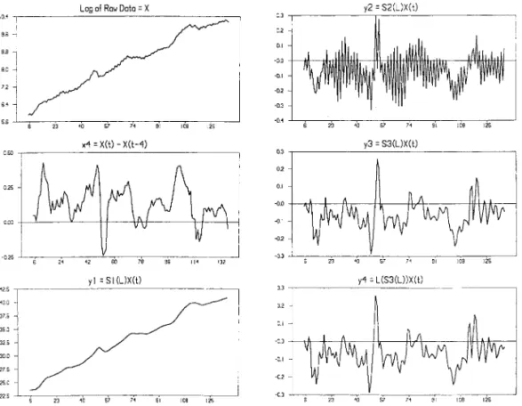
exception of r1, all variables are in natural logarithms. Fig. 1᎐7 plots the seven
variables with their seasonal transformations.
Table 1 presents the HEGY seasonal unit root tests. The lag length listed, which is designed to remove autocorrelation from the residuals, is based on the Akaike
Ž .
information criterion AIC . According to the table, the t-values for the null
hypothesis of s 0 for all variables are smaller than the 5% critical values listed1
5
Ž . Ž .
Hence, Y3 ty1 and Y4 ty1 in 9 correspond to y3 ty2and y3 ty1in 8 , respectively. 6
Ž .
The test of seasonal frequency at s 1r4, as noted by Lee 1992 , is tested on the matrix ⌸ only on3
Fig. 1. Real reserve and its seasonal transformation.
in HEGY regardless of the deterministic components. Thus, the null of the seasonal unit root at zero frequency is accepted by all variables in question. In
addition, the t-statistic for s 0 is rejected for r, ex, p, r1 and , but cannot be2
rejected for M1B, M2 and y. However, for im, s 0 is rejected when seasonal2
dummies are excluded; but it is accepted when the same dummies are included. As
Ž .
Osborn et al. 1988 stated, the inclusion of seasonal dummies when testing for seasonal unit roots is important; otherwise, variables tend to display stochastic seasonality even when they contain only deterministic seasonality. Thus, we can conclude that im contains a seasonal unit root at the biannual frequency. The
hypothesis of s s 0 cannot be rejected only for the cases of r and y. Except3 4
for im and y, the hypothesis of s s s 0 and s s s s 02 3 4 1 2 3 4
are rejected for all variables. Since t-tests display conflicting evidence against
F-tests, we have to decide which one to use. We prefer to use t-tests because their
results are consistent with the stylized fact that conventional unit roots exist in the most macro series. However, further research is needed to pursue this issue.
In summary, all series under consideration are non-stationary at zero frequency. Ž .
Although the logarithm of real GNP y presents seasonal unit roots at additional
Fig. 2. Real GNP and its seasonal transformation.
1r2 or 1r4 frequency.
Ž .
Let notation x i, i, i denote whether or not the variable x has unit roots at
either zero, 1r2 or 1r4 frequencies, respectively. If i s 1, there is a unit root at
the corresponding frequency, otherwise, if is 0 it is not. Hence, we can infer the
following from Table 1:
Ž . Ž . Ž . Ž . Ž . Ž . Ž . Ž .
1. C, T : M1B 1,1,0 , M2 1,1,0 , r 1,0,0 , ex 1,0,0 , cpi 1,0,0 , r1 1,1,0 , im 1,0,0 ,
Ž . Ž .
y 1,1,1 , 1,0,0
Ž . Ž . Ž .
2. C, SD and C, T, SD : except for im 1,1,0 , other variables are the same as above.
4.2. The demand for money and seasonal cointegration
Since money market disequilibrium is one of the crucial determinants in the
demand for reserves and since it contains seasonal unit root at the 1r2 frequency,
its projected values should be obtained on the basis of the SECM specification. Table 2A,B summarize the seasonal cointegration testing results for M1B and M2, respectively. The deterministic components, C, T, and SD, will be included in
Fig. 3. Real M2 and its seasonal transformation.
the statistical models if they are significant. Since the finite sample quantiles
Ž .
provided by Lee 1992 do not consider any of the deterministic components, the quantile distributions by Monte Carlo simulations are computed here using 30 000 replications with deterministic terms contained in the statistical models.
Table 2A reveals that the five variables, M1B, y, r1, ex, and p are all
cointegrated at the zero frequency.7 The corresponding normalized vector of
Ž .
cointegrating coefficients,  , is 1, y4.5800, 0.0929, 0.9793, 0.6870 . Both signs1
and magnitudes agree well with existing monetary studies. Namely, income has a positive effect, and the interest rate, exchange rate and inflation rate negatively impact the demand for money.
Since five series are used in the VAR system, there are five error correction terms. The coefficients on these five terms are represented by the vector of
Ž .
␣ s y0.0067, 0.0013, y0.0836, 0.0027, y0.0021 , which are interpreted as the1
7
We have examined whether the residuals of above equations are normal or not. Results show that only
y and r pass the normality tests of Bera᎐Jarque. However, errors with non-Gaussian distributions will Ž . not substantially alter the properties owned by the maximum likelihood estimators, as Gonzalo 1994 has pointed out.
Fig. 4. Real MIB and its seasonal transformation.
average speeds of adjustment towards the long-run equilibrium or the loadings
ŽJohansen and Juselius, 1990 . A negative number indicates that when an excess.
demand or supply occurs, market forces will eliminate the disequilibrium and bring
the system back to a steady state. The first element of ␣ corresponds to the1
adjustment speed for the monetary disequilibrium and is roughly y0.0067. Thus,
the excess demand for money will be at least partially adjusted downward in the next period, so that disequilibrium in the money market would be eliminated eventually.
Since only M1B and y contain seasonal unit roots at the 1r2 frequency, Lee’s
seasonal cointegration test is again applied to these two series only. The two series are discovered to be cointegrated at this frequency with cointegrating vector
Ž .
 s 1, y0.8742 . This income elasticity is smaller than that at zero frequency,2
implying that a seasonal increase in income would have a smaller effect on money holding than an increase in income at zero frequency. The adjustment speed of the
money market at the 1r2 frequency, which is equal to 0.0073, is the first element of
␣ in Table 2A. This non-negative number, contrary to the result at the zero2
frequency, does not imply the adjustment will make the system gradually deviate
Ž .
Fig. 5. One month rate and its seasonal transformation.
seasonal error correction terms can be positive even if the adjustment is heading
Ž . 8
toward equilibrium at seasonal frequencies. Lee 1992 provides a similar report. However, the economic meaning of a positive loading is unclear.
In Table 2B, two long-run equilibrium relationships among the five series, M2, y,
r1, ex, and p are discovered. Though the elements of the two cointegrating vectors,
 and  , differ in magnitudes, they have the same signs thereby corresponding to1 2
the predictions of the existing monetary theories. The speed of adjustment of M2
error corrections corresponding to the two long-run equilibrium errors arey0.0056
and y0.0040, respectively. Interestingly, those numbers are smaller than that in
M1B, indicating that the adjustment speed towards steady state is slower for the broad money than for the narrow money. This appears to be reasonable since M2 contains both transaction and saving assets and, thus, is less liquid than M1B, which contains mainly transaction assets.
8
Ž .
Lee 1992 examined the existence of seasonal cointegration relations at different frequencies using quarterly data on unemployment and immigration rates from Canada. The coefficient on the seasonal error correction term at 1r2 frequency was also positive.
Fig. 6. Real import and its seasonal transformation.
The seasonal cointegration test is again applied to M2 and y only at the 1r2
frequency, since only these two series contain a seasonal unit root at the frequency.
Ž .
The normalized income elasticity is 0.84 and the loading isy0.0017.
Since only y contains unit root at the frequency 1r4, testing the seasonal
cointegration at this frequency is not necessary.
Once the seasonal cointegrating vectors are detected for the two measures of
money aggregates, the next step is to derive the linear projectors ⌬ m4
ˆ
ty4 and⌬2m . This can be achieved by estimating the SECM with the seasonally differ-
ˆ
4 tenced money aggregates as dependent variables and the lagged fourth order seasonally differenced explanatory variables in the model. The seasonal error correction terms are also included on the right hand side of the regression equation. The estimated results of the two SECMs are not presented, but are available upon request. Their linear projections then function as explanatory
Ž . variables and are included in Eq. 5 .
4.3. The estimation of demand for international reser¨es
Ž . Ž
Fig. 7. Reserve-uncertainty and its seasonal transformation.
.
intercept be cointegrated at the conventional frequency. This conjecture can be tested by means of Johansen’s maximum likelihood procedure. The two test
Ž .
statistics of Johansen’s method, -max the maximal eigenvalue statistic and the
trace statistics, lead to the same conclusion of one cointegrating relationship
among the four series.9 The equilibrium error term, which is a stationary process,
can be written as
Ž .
ECty1s rty1y 1.9024 yty1y 0.1742imty1y 0.2174ty1q 21.7767 10
where the cointegrating coefficients reveal that y, im and positively influence
the demand for reserves.
Once the ECty1 is obtained, it will be treated as an explanatory variable in Eq.
Ž .5 . Hence, estimating Eq. 5 by OLS is now free of the criticism of spuriousŽ .
regression since all variables are now stationary. Ž .
Notably, Eq. 5 may be still misspecified by omitting the seasonal error
correc-Ž .
tion terms if these exist . More specifically, since seasonal unit roots exist at the
Table 1
HEGY seasonal unit root test: t-values
t1 t2 F34 F234 F1234 Ž . 1. M1B lags 4, N s 126 a a a C,T y3.133 y1.142 20.898 14.721 13.266 a a a C,T,SD y3.288 y2.981 23.656 21.393 18.503 Ž . 2. M2 lags 5, N s 125 a a a C,T y3.450 y1.527 18.930 13.381 15.100 a a a C,T,SD y3.258 y2.668 22.485 17.071 18.114 Ž . 3. r lags 1, N s 130 a a a a C,T y2.180 y6.391 40.771 54.157 49.435 a a a a C,T,SD y2.154 y6.335 39.762 52.991 48.378 Ž . 4. ex lags 0, N s 133 a a a a C,T y2.751 y6.867 89.779 213.75 167.60 a a a a C,T,SD y2.733 y6.736 91.649 219.21 171.81 Ž . 5. p lags 0, N s 133 a a a a C,T y1.710 y8.015 71.210 253.94 190.73 a a a a C,T,SD y1.726 y7.730 72.888 255.84 192.16 Ž . 6. r1 lags 0, N s 133 a a a a C,T y3.142 y9.336 46.465 361.26 274.60 a a a a C,T,SD y3.143 y9.367 45.146 362.83 275.77 Ž . 7. im lags 5, N s 128 b a a a C,T y1.676 y2.301 7.607 6.799 5.883 a a b C,T,SD y1.670 y2.475 10.820 9.151 7.673 Ž . 8. y lags 5, N s 128 b C,T y1.200 y1.847 2.750 2.996 2.667 C,T,SD y1.167 y1.452 3.131 2.794 2.519 Ž . 9. lag s 0, N s 117 a a a a C,T y3.085 y5.711 22.057 27.904 22.955 a a a a C,T,SD y3.061 y5.665 21.740 27.486 22.596
aSignificant at the 1% level. bSignificant at the 5% level.
Ž w x Ž .
Critical value taken from HEGY and Ghysels 1994 .
Ž .
5% Ns 136 for t , t , F and N s 100 for F1 2 34 234and F1234 C, T y 3.46 y 1.96 3.04 2.76 4.26 C, T, SD y 3.52 y 2.93 6.62 5.99 6.47 Ž . 1% Ns 136 C, T y4.09 y 2.65 4.57 na na C, T, SD y 4.15 y 3.57 8.77 na na
1r2 andror 1r4 frequencies for the series y, im, and r, they may be cointegrated
at those frequencies. If cointegrating relationships indeed exist at the 1r2 or 1r4
frequencies, then the conventional ECM models, such as those used by Elbadawi
Ž1990 , Johansen and Juselius 1990 , and Ford and Huang 1994 among others,. Ž . Ž .
Table 2
Seasonal cointegration test A: M1B Money demand function
Ž . ⌬ X s C q C T q4 t 0 1 SD q ⌸ Yt 1 1,ty1q ⌸ Y2 2,ty1q ⌸ Y3 3,ty1q ⌸ Y4 4,ty1q A L ⌬ X q4 t ⑀t
Frequency Ranks 0 Ranks 1 Ranks 2 Ranks 3 Ranks 4 b s 0 96.293 60.251 26.411 7.334 0.289 a s 1r2 33.932 3.731 Ž . Eigenvectors  Error-correction Ž . coefficients ␣ Zero frequency 1r2 frequency
1 ␣1 2 ␣2
M1B 1 y0.0067 1 0.0073
y y4.5800 0.0013 y0.8742 y0.0027
r1 0.0929 y0.0836 y0.0046
ex 0.9793 0.0027 y0.0020
p 0.6870 y0.0021 0.0028
Ž .
M1B critical values Ns 136, generated by the authors
s 0 ny r s 5 ny r s 4 ny r s 3 ny r s 2 ny r s 1 95% 87.442 61.747 40.994 24.349 11.755 99% 96.339 69.695 47.502 27.694 15.770 s 1r2 95% 18.488 8.238 99% 23.356 12.119
B: M2 money demand function
Ž .
⌬ X s C q C T q ⌸ Y4 t 0 1 1 1,ty1q ⌸ Y2 2,ty1q ⌸ Y3 3,ty1q ⌸ Y4 4,ty1q A L ⌬ X q4 t ⑀t
Frequency Ranks 0 Ranks 1 Ranks 2 Ranks 3 Ranks 4 s 0 103.968a 62.808b 30.712 6.058 0.151
a
s 1r2 21.293 2.351
Ž . Ž .
Eigenvectors  and error-correction coefficients ␣
Zero frequency 1r2 frequency
11 12 ␣11 ␣12 2 ␣2
M2 1 1 y0.0056 y0.0040 1 y0.0017
y y5.0895 y1.6585 y0.00033 0.0031 y0.8427 y0.0018
r1 0.1685 0.0169 y0.2299 y0.0347 y0.0083
ex 1.0525 0.5000 0.0086 y0.0094 y0.0050
p 0.7775 0.6664 y0.0043 0.0020 0.0054
aSignificant at the 1% level. bSignificant at the 5% level.
The critical values of M2 are close to those of M1B and are available from authors.
Table 3 summarizes the testing results. Similar to Table 2A,B, the finite sample quantile distributions are calculated by Monte Carlo simulations using 30 000
replications. At the 1r2 frequency, y and im are found to be cointegrated with the
equilibrium error process as:
Ž . Ž . Ž .
Table 3
Demand for international reserves equations: seasonal cointegration test model:⌬ X s C q4 t 0 D qt Ž .
⌸ Y1 1,ty1q ⌸ Y2 2,ty1q ⌸ Y3 3,ty1q ⌸ Y4 4,ty1q A L ⌬ X4 ty1q⑀t
Frequency Ranks 0 Ranks 1 Ranks 2 Ranks 3
b s 0 53.149 29.026 11.379 1.654 a s 1r2 27.396 4.721 s 1r4 19.951 4.497 Eigenvectors at Eigenvectors at s 0 s 1r2 r 1 y y1.7279 1 y0.3956 im 3.4126 0.2325 Ž .
Critical values Ns 100, critical values are generated by the authors
s 0 ny r s 4 ny r s 3 ny r s 2 ny r s 1 95% 52.358 33.125 18.350 8.287 99% 59.886 37.449 23.002 11.885 s 1r2 95% 18.406 8.293 99% 23.361 11.907 s 1r4 95% 23.312 11.365 99% 28.768 15.771
aSignificant at the 1% level. bSignificant at the 5% level.
D is the centered seasonal dummies.t
Ž .
A L⌬ X4 ty1 is the lagged seasonal difference, lag:5.
N is the sample size.
where the subscript 2 denotes 1r2 frequency. In contrast, no cointegration
rela-tionships are found between y and r at the 1r4 frequency. Accordingly, only
Ž .
SEC2, ty1 is used as an extra variable in Eq. 5 .
Table 4 reports the estimation results of the seasonal cointegration specification
Ž .5 with the term SEC2, ty1 being added to the conventional cointegration
specifica-Ž .
tion 6 . Furthermore, both measures of monetary aggregates are employed. For each specification, all estimated coefficients have the same signs and similar magnitudes, regardless of which monetary aggregate is used. This fact implies that the level of reserve holdings is unaffected by different definitions of monetary
disequilibria. While the estimated coefficients for the ECty4 and ECty1 have
anticipated negative signs; their absolute values are all small, ranging fromy0.056
toy0.033. Such a low speed of adjustment is quite different from pervious studies
Ž .
in this area. For instance, Elbadawi 1990 obtained a high adjustment coefficient
Table 4
Estimates of the demand for international reserves
SECM ECM
Independent ⌬ r4 t ⌬ r4 t Independent ⌬rt ⌬rt
Ž . Ž . Ž . Ž .
variable M1B M2 variable M1B M2
UU UUU UU
ECty4 y0.0331 y0.0501 ECty1 y0.0558 y0.0462
Ž0.0243. Ž0.0260. Ž0.0201. Ž0.0186.
U UUU UU
⌬ m4ˆty4 y0.2229 y0.2419 ⌬mˆty1 0.6576 0.7778 Ž0.1198. Ž0.1972. Ž0.2032. Ž0.1958.
UU U
SEC2,ty1 y0.0269 y0.0230 Ž0.0123. Ž0.0130.
UUU UU
⌬ y4 t 0.5232 0.5557 ⌬ yt y0.0227 y0.2154
Ž0.1841. Ž0.2831. Ž0.2268. Ž0.1999.
UUU UU UU
⌬ im4 t y0.1130 y0.2098 ⌬imt y0.1244 y0.1174
Ž0.0749. Ž0.0809. Ž0.0627. Ž0.0580. ⌬4t 0.0018 0.0024 ⌬t 0.0028 0.0021 Ž0.0029. Ž0.0033. Ž0.0027. Ž0.0025. 2 UU UUU UUU 2 ⌬ m4ˆt y0.2199 y0.1965 ⌬ mˆt 0.5064 0.9473 Ž0.0897. Ž0.1334. Ž0.1352. Ž0.1625. 2 adj-R 0.9260 0.9156 0.3906 0.4769 Ž . Ljung᎐Box Q 10 3.01 11.17 5.07 6.10 Ž . Ljung᎐Box Q 20 11.81 23.99 22.66 15.53 Ž . ARCH 1 0.94 0.15 0.23 0.73
Jarque᎐Bera 2.56 2.06 13.12UUU 26.85UUU
Normality test
UUU UU
Chow Test 1.20 0.96 2.53 2.24
U,UU, andUUU: significant at the 10, 5 and 1% level, respectively. Standard errors in parentheses.
Note. The estimated coefficients of lagged dependent variables on the right hand side of the above
equations are not reported for the sake of space. The lags are 10, 9, 6, and 6 for the above four equations from left to right, respectively. The Chow test is based on the splitting point 1986:1, see text and the corresponding footnote.for details.
Ž .
y0.81 and y0.52 were derived by Ford and Huang 1994 employing annual narrow and broad monetary aggregates, respectively, from mainland China.
The low adjustment speed of Taiwan’s demand for reserves could be accounted
Ž . Ž .
for by the theory of Clark 1970a . As contended by Clark 1970a , a tradeoff arises between the speed of adjustment and the level of reserves held by a country. A country with a lower speed of adjustment heading towards equilibrium requires a higher level of reserves as a buffer stock to finance its payments problems and vice
versa. Since Taiwan is well-known for its huge stock of international reserves,10the
10
The balance-of-payment surplus of Taiwan amounted to $US90 billion at the end of 1993, which was the second largest globally.
low speed of adjustment appears to be reasonable. The coefficient estimates of the
term SEC2, ty1 are negative and significant, at least at the 10% level, indicating
that the conventional EC model may be inhibited by model misspecification. While the money market disequilibria are found to have significantly negative effects on the demand for reserves in the seasonal specification, the results are reversed in the conventional EC models. Recall that the effect of money market disequilibrium on the demand for reserves is uncertain. Namely, the monetary approach suggests a positive effect, whereas a reconciliation argument postulates a negative effect. Thus, the negative effect yielded by the seasonal specification favors the latter explanation, whereas the positive effect yielded by the conventio-nal specification supports the former. To clarify which specification is preferable, diagnostic checks can provide valuable insight and will be implemented shortly.
Ž .
Income y is found to have a significantly positive as expected effect on the demand for reserves in the seasonal model, but is found lacking in the conventional
model. Both models indicate that variability has no effect on reserve movements.
The coefficients on the average propensity to import im are all negative; neverthe-less, all of them are statistically insignificant.
The diagnostic checks are reported in the bottom panel of Table 4. Since these test statistics can be found in the most econometric textbooks, introductions of their definitions are omitted to save space.
Ž . Ž .
Both specifications pass the Ljung᎐Box Q 10 and Q 20 tests for no residual
autocorrelation, where numbers in the parentheses denote the numbers of lagged autocorrelations. Also, no ARCH effect is detected regardless of the specifications. However, the conventional specification fails, but the seasonal specification passes,
both the Jarque᎐Bera normality test and the Chow parameter stability test.11
Finally, the adjusted R2 is higher for the seasonal model than the conventional
model, suggesting a better fit for the former. Thus, on the basis of the above diagnostics, the seasonal specification appears to be preferable to the conventional one.
4.4. The structural parameters
The size of the income elasticity has attracted much attention in previous studies involving demand for reserves. The elasticity, which may be greater than, equal to, or less than unity, indicates the diseconomies, constant economies and economies of scales in holding reserves, respectively. This elasticity may be calculated by
Ž .
recovering the structural parameters in Eq. 4 from the reduced form parameters
listed in Table 4. For instance, the structural parameter is simply the absolute1
11Selecting a breaking point for the Chow test is based on preliminary checking of the plots of the
Ž . Ž .
cumulative sum CUSUM and cumulative sum of squares CUSUMSQ test. These two plots, which are not reported here, but are available upon request, display a tendency for breaking at 1977 and 1986.
Ž .
Selecting any breaking point between these two dates there are 40 splits in total , the Chow test overwhelmingly rejects the null of no structural break for the conventional specification. By contrast, the null cannot be rejected for the seasonal specification. The Chow tests reported in Table 4 uses the breaking point 1986.
Table 5
Reserved structural parameters
Parameter Seasonal model Conventional model
⌬ r4 t ⌬ r4 t ⌬rt ⌬rt ŽM1B. ŽM2. ŽM1B. ŽM2. UUU UU a1 16.0255 13.6460 y0.5277 y3.8250 Ž5.6382. Ž6.9521. Ž5.2798. Ž3.5496. a2 0.0539 0.0593 0.0656 0.0376 Ž0.0884. Ž0.0800. Ž0.0621. Ž0.0439. UUU UU UU
a3 y3.4609 y5.1519 y2.8963 y2.0853
Ž2.2953. Ž1.9872. Ž1.4585. Ž1.0298. UU UU a4 y6.7357 y4.8258 11.7875 16.8220 Ž6.5256. Ž4.7103. Ž5.2121. Ž7.7754. UU UUU UU 1 0.0331 0.0501 0.0558 0.0462 Ž0.0243. Ž0.0260. Ž0.0201. Ž0.0186. UU UUU UUU 2 0.0326 0.0407 0.0430 0.0563 Ž0.0133. Ž0.0276. Ž0.0115. Ž0.0097. U,UU, andUUU: significant at the 10, 5 and 1% level, respectively.
Standard error in parenthesis.
value of b . The structural parameter1 is obtained by calculating b ra where2 6 4
a4s b r . The remaining structural parameters can be recovered using the same2 1
manner and are reported in Table 5 for both specifications.
Once the structural parameters are recovered, the null hypothesis of a unitary income elasticity can be tested. The null is
H :a0 1y 1 s b r y 1 s 03 2
Since a is 16.03 or 13.65 when M1B or M2 disequilibrium is incorporated in the1
seasonal specifications, respectively, the null hypothesis is rejected. The demand for international reserves by Taiwan thus faces strong diseconomies of scale. In
contrast, a has a wrong negative sign in the conventional specification. This1
finding again suggests that the seasonal model is preferable to the conventional model.
The above diseconomies may be attributed to various regulations imposed on the holding of foreign exchange. Prior to 1986, civilians in Taiwan could buy foreign exchange only with the permission of the monetary authorities for a limited amount annually and for some pre-specified purposes. Firms had to sell their foreign exchange, earned by exporting goods and services, to the central bank. These restrictions have been gradually lifted since 1986 and are now a self-fueled ongoing processes for the Central Bank. Similar strong diseconomies of scale were
Ž . Ž .
Ž .
found the income elasticity to be only 0.687, while Elbadawi 1990 accepted the null of constant returns to scale.
5. Concluding remarks
On the basis of a conventional one-period loss function involving official growth rate computed from seasonal differences, a dynamic demand function for interna-tional reserves is derived. This small modification distinguishes the present study from previous studies in three aspects. First, the dependent variable is seasonally differenced instead of being first order differenced. Next, the local money market disequilibrium included is also in fourth difference form. Finally, given the exis-tence of stochastic seasonality, a new model, using a seasonal error correction rather than the conventional error correction, is specified and estimated. The following inferences are drawn from the seasonal specification.
1. Regarding the demand for a money equation, a long-run equilibrium relation-ship exists at the zero frequency among money, income, the exchange rate, and the price level. Moreover, money and income are seasonally cointegrated at the biannual frequency.
2. With respect to the demand for international reserves, a long-run relationship is discovered among reserves, income, the average propensity to import, and a measure of the variability in the balance of payments at the zero frequency. Also, income and the average propensity to import are seasonally cointegrated at the biannual frequency.
3. The current period’s change in income has a significantly positive effect on reserve holdings in the short-run, but is smaller in magnitude than its long-run counterpart.
4. The monetary authorities of Taiwan respond quite slowly to deviations from the desired demand for reserves occurring four periods before. This is most likely due to regulations imposed on private reserve holdings on the one hand, as well as a tradeoff between the speed of adjustment and the stock of reserves a country is willing to hold on the other.
Ž .
5. While the narrow money market disequilibrium M1B displays a short-run
Ž .
effect on the demand for reserves, the broad money market disequilibrium M2 exerts no significant influences on the reserve holdings in both the short- and long runs.
6. The precautionary motive is found to be an unimportant determinant of the demand for reserves, possibly due to the fact that Taiwan has accumulated a
Ž
large stock of foreign exchange during the past two decades relative to its trade .
flows and, therefore, the risk of an external payment problems would be very low.
7. Since the equilibrium error from the biannual frequency significantly affects the demand for reserves, it has to be incorporated in the seasonal EC model. This term is neglected in the conventional EC model.
References
Abeysinghe, T., 1991. Inappropriate use of seasonal dummies in regression. Econ. Lett. 36, 175᎐197. Clark, P.B., 1970a. Optimum international reserve and the speed of adjustment. J. Polit. Econ. 78,
356᎐376.
Clark, P.B., 1970b. Demand for international reserve: a cross-country analysis. Can. J. Econ. 3, 577᎐594. Clower, R., Lipsey, R., 1968. The present state of international liquidity theory. Am. Econ. Rev. 58,
586᎐595.
Edwards, S., 1984. The demand for international reserves and monetary equilibrium: some evidence from developing countries. Rev. Econ. Stat. 66, 496᎐500.
Elbadawi, I.A., 1990. The Sudan demand for international reserve: a case of a labor-exporting country. Economica 57, 73᎐89.
Engle, R.F., Granger, C.W.J., 1987. Cointegration and error correction: representation, estimation and testing. Econometrica 55, 251᎐276.
Engle, R.F., Granger, C.W.J., Hallman, J., 1989. Merging short- and long-run forecasts: an application of seasonal co-integration to monthly electricity sales forecasting. J. Econom. 40, 45᎐62.
Engle, R.F., Granger, C.W.J., Hylleberg, S., Lee, H.S., 1992. Seasonal cointegration: the Japanese consumption function. J. Econom. 55, 275᎐298.
Ericsson, N., Hendry, D.F., Tran, H., 1994. Cointegration, seasonality, encompassing and the demand Ž .
for money in the United Kingdom. In: Hargreaves, C.P. Ed. , Nonstationary Time Series Analysis and Cointegration. Oxford University Press, New York, pp. 85᎐101.
Ford, J.L., Huang, G., 1994. The demand for international reserves in China: an ECM model with domestic monetary disequilibrium. Economica 67, 379᎐397.
Ž .
Frenkel, J.A., 1974. Openness and the demand for international reserve. In: Aliber, R.Z. Ed. , National Monetary Politics and the International Financial System. University Press, Chicago.
Ž . Frenkel, J.A., 1983. International liquidity and monetary control. In: von Furstenberg, G.M. Ed. ,
International Money and Credit: The Policy Roles. IMF, Washington D.C.
Ghysels, E., 1994. On the periodic structure of the business cycle. J. Bus. Econ. Stat. 12, 289᎐298. Ghysels, E., Lee, H.S., Noh, J., 1994. Testing for unit roots in seasonal time series: some theoretical
extensions and a Monte Carlo investigation. J. Econom. 62, 415᎐442. Ž .
Ghysels, E., Lee, H.S., Siklos, P.L., 1993. On the Mis specification of seasonality and its consequences: an empirical investigation with US data. Empirical Econ. 18, 747᎐760.
Gonzalo, J., 1994. Five alternative method of estimating long-run equilibrium relationships. J. Econom. 60, 203᎐233.
Grubel, H.G., 1969. The International Monetary System. Penguin Books, New York.
Hargreaves, C., 1994. A review of methods of estimating cointegrating relationships. In: Hargreaves, Ž .
C.P. Ed. , Nonstationary Time Series Analysis and Cointegration. Oxford University Press, New York, pp. 87᎐132.
Heller, H.R., Khan, M.S., 1978. The demand for international reserve under fixed and floating exchange rates. IMF Staff Paper 25, 623᎐649.
Heller, R.H., 1966. Optimal international reserves. Econ. J. 76, 296᎐311.
Hendry, D.F., Sternberg, T.V., 1981. Liquidity and inflation effects on consumers’ expenditure. In: Ž .
Deaton Ed. , Essays in the Theory and Measurement of Consumer’s Behavior. University Press, Cambridge, pp. 18᎐24.
Hylleberg, S., Engle, R.F., Granger, C.W.J., Yoo, B.S., 1990. Seasonal integration and cointegration. J. Econom. 44, 215᎐238.
Johansen, S., 1988. Statistical analysis of cointegration vectors. J. Econ. Dynam. Control 12, 231᎐254. Johansen, S., Juselius, K., 1990. Maximum likelihood estimation and inference on cointegrationᎏwith
applications to the demand for money. Oxf. Bull. Econ. Stat. 52, 169᎐210.
Kenen, P.B., Yudin, E.B., 1965. The demand for international reserves. Rev. Econ. Stat. 47, 242᎐250. Lee, H.S., 1992. Maximum likelihood inference on cointegration and seasonal cointegration. J. Econom.
54, 1᎐47.
McKinnon, R.I., Oates, W.E., 1966. The Implications of International Economic Integration for Monetary, Fiscal and Exchange Rate Policy. No. 16, Princeton University, Studies in International Finance.
Osborn, D.R., Chui, A.P.L., Smith, J.P., Birchenhall, C.R., 1988. Seasonality and the order of integration for consumption. Oxf. Bull. Econ. Stat. 50, 361᎐377.
Shen, C.-H., Huang, T.-H., 1998. Seasonal cointegration and money demand: the case of Taiwan, Int. Econ. J., forthcoming.