具有AR(1)誤差的迴歸模型的線性修正平均估計值

全文

(1)國立交通大學統計學研究所碩士論文. 具有 AR(1)誤差的迴歸模型的線性修正平均值估計 Linear Trimmed Means for the Linear Regression with AR(1) Errors Model. 研究生：彭豐洋指導教授：陳鄰安博士. 中華民國九十四年六月.

(2) 具有 AR(1)誤差的迴歸模型的線性修正平均值估計 Linear Trimmed Means for the Linear Regression with AR(1) Errors Model. 研究生：彭豐洋. Student：Feng-Yang Peng. 指導教授：陳鄰安博士. Advisor：Dr. Lin-An Chen. 國立交通大學理學院統計研究所碩士論文. A thesis Submitted to Institute of Statistics College of Science National Chiao Tung University In partial Fulfillment of the Requirements For the Degree of Master in Statistics June 2005 Hsinchu Taiwan Republic of China. 中華民國九十四年六月.

(3) 具有 AR(1)誤差的迴歸模型的線性修正平均值估計. 研究生：彭豐洋指導教授：陳鄰安博士國立交通大學統計研究所. 中文摘要延續 Lai (2003)其具有 AR(1)誤差的線性迴歸模型的穩健性估計基本架構，我們證明了在大樣本的情形下廣義修正平均值估計量能夠有類似 Gauss Markov Theorem 的性質。我們稱其為穩健型態的 Gauss Markov Theorem。我們進而利用模擬的方法以及實例的分析，說明該估計量的特性與效率。.

(4) Linear Trimmed Means for the Linear Regression with AR(1) Errors Model. Student: Feng-Yang Peng. Advisor: Dr. Lin-An Chen. Institute of Statistics, National Chiao Tung University, Hsinchu, Taiwan.. Abstract For the linear regression with AR(1) errors model, a robust type generalized and feasible generalized estimators of Lai et al. (2003) of regression parameters are shown to have the desired property of robust type Gauss Markov theorem. It is done by shown that these two estimators are, respectively, the best among classes of linear trimmed means. Monte Carlo and data analysis for this technique have been performed.. Keywords: Gauss Markov theorem; Generalized least squares estimator; linear trimmed mean; robust estimator..

(5) 誌謝感謝指導老師陳鄰安教授孜孜不倦地教導，本論文方能順利完成。承蒙交通大學彭南夫教授、清華大學統計學研究所徐南蓉教授與江永進教授於百忙之中撥冗審稿、校正，並給予寶貴的意見，僅此表達誠摯的謝忱。感謝所上諸位老師的指導，郭姐的照顧，以及一起研究的同伴們，育仕、景嵐、穎劭、雅靜、玉均、辰昀、揚波、婉菁、瑩琪等，對我的鼓勵與包容。感謝媽媽、姊姊陪我一路走來，無怨無悔的付出所有愛與關懷，有你們的支持我才成克服一切的困難，沒有後顧之憂地完成我的學業。僅將本論文獻給各位。. 彭豐洋. 僅誌于. 國立交通大學統計研究所中華民國九十四年六月.

(6) Contents 1.. Introduction. 1. 2.. Linear Trimmed Mean When ρ is known. 3. 3.. Asymptotic Properties of Linear Trimmed Mean. 6. 4.. Linear Trimmed Means When ρ is Unknown. 9. 5.. Monte Carlo Study and Example. 10. 6.. Appendix. 13. Reference. 15.

(7) 1. Introduction Consider the linear regression model y = Xβ + ². (1.1). where y is a vector of observations for the dependent variable, X is a known n × p design matrix with 10 s in the first column, and ² is a vector of independent and identically distributed disturbance variables. We consider the problem of estimating the parameter vector β and the parametric function c0 β of β. From the Gauss-Markov theorem, it is known that the least squares estimator has the smallest covariance matrix in the class of unbiased linear estimators M y where M satisfies M X = Ip . Also, the inner product of c and the least squares estimator has smallest variance among all linear unbiased estimators of c0 β. However, the least squares estimator is sensitive to departures from normality and to the presence of outliers so we need to consider robust estimators. An interesting question in robust regression is if there is robust type Gauss-Markov theorem, i.e., if there is a robust estimator that is (asymptotically) more efficinet than a class of linear robust estimators? This has been done by Chen et al. (2001) that they considered a class of estimators based on Winsorized observations and show that the trimmed mean of Welsh (1987) is asymptotically the best among it. Suppose that the error vector ² = (²1 , ..., ²n )0 has the covariance matrix structure Cov(²) = σ 2 Ω. (1.2). where Ω is a positive definite matrix. From the regression theory of the estimation of β, it is known that any estimator having an (asymptotic) covariance matrix of the form δ(X 0 Ω−1 X)−1. (1.3). is more efficient than the estimator having (asymptotic) covariance matrix of the form δ(X 0 X)−1 (X 0 ΩX)(X 0 X)−1. (1.4). where δ is some positive constant. In the least squares estimation when the matrix Ω is known, Aitken (1935) introduced the generalized least squares estimator (LSE) and 1.

(8) 2. showed that it has a covariance matrix of the form (1.3) and the LSE has a covariance matrix of the form (1.4) with δ = σ 2 . It is also well known that, when Ω is unknown, the feasible generalized LSE has the asymptotic covariance matrix of the form (1.3). Then these two generalized type estimators are more efficient than the LSE. Although the generalized and feasible generalized LSE’s are asymptotically more efficient than the LSE in many regression problems, they are highly sensitive to even a very small departure from normality and to the presence of outliers. Therefore developing robust type generalized and feasible generalized estimators in each specific regression problem is interesting. Let’s consider the linear regression with AR(1) errors model, a structure of (1.2), as follows yi = x0i β + ²i , i = 1, ..., n ²i = ρ²i−1 + ei. (1.5). where e1 , ..., en are independent and identically distributed (iid) random variables, is one of the most popular models. Suppose that |ρ| < 1 and ei has a distribution function F . 0. Denote the transformed vector u = Ω−1/2 y. One approach to robust estimation is to construct a weighted observation vector u∗ and then construct a consistent estimator which is linear in u∗ , in case that ρ is unknown, all vectors are replaced by the ones with estimating ρ by estimator ρˆ; see for example, Lai et al. (2003). There are two types of weighted observation vectors in this literature. First, u∗ can represent a trimmed observation vector Au with A a trimming matrix constructed from regression quantiles (see Koenker and Bassett (1978)), or residuals based on an initial estimator (see Ruppert and Carroll (1980) and Chen (1997)). Second, u∗ can be a Winsorized observation vector defined as in Welsh (1987). In this paper, we consider the trimmed observation vector of Koenker and Bassett (1978), study classes of linear functions based on u∗ for estimation of β, and develop a robust version of the Gauss-Markov theorem. Based on regression quantiles, Lai et al. (2003) proposed generalized and feasible generalized trimmed means for estimating regression parameters β. Then a robust type generalized and feasible generalized estimation technique have been developed. With the result that we have robust version of Gauss Markov theorem for linear regression with iid errors model, it is then interesting to see if there is any robust type.

(9) 3. generalized and feasible generalized estimators for the linear regression with AR(1) errors model that also play the same version of Gauss Markov theorem. Our aim in this paper is to show that the Lai et al. (2003) does have this desired property. We introduce a class of linear trimmed means when ρ is known in Section 2 and establish their large sample theory in Section 3. We also establish the theory for a class of linear trimmed means when ρ is unknown in Section 4. In both cases, we show that the generalized and feasible generalized trimmed means are the best, respectively, in these two classes of linear trimmed means in terms of asymptotic covariance matrix. Finally, the proofs of the theorems are displayed in Appendix. 2. Linear Trimmed Mean When ρ is known For the linear regression with AR(1) errors model (1.5), to obtain a linear trimmed mean we need to specify the quantile for determining the observation trimming and to make a transformation of the linear model to obtain generalized estimators. For given i-th dependent variable for model (1.5), assuming that i ≥ 2 , one way to derive a generalized estimator is to consider the transformation by Cochrane and Orcutt (C-O, 1949) as yi = ρyi−1 + (xi − ρxi−1 )0 β + ei . For error variable e, we assume that it has distribution function F with probability density function f . With the transformation for generalized estimation, a quantile could be defined through variable e or a linear conditional quantile of yi−1 and yi . By the fact that xi is vector with first element 1, the following two events determined by two quantiles are equivalent: ei ≤ F −1 (α) and. µ (−ρ, 1) µ. with β(α) = β +. 1 −1 (α) 1−ρ F 0p−1. yi−1 yi. ¶. (2.1) µ. ≤ (−ρ, 1). x0i−1 x0i. ¶ β(α). (2.2). ¶ . The event in inequality (2.1) specifies the quantile of. the error variable e andµit through inequality (2.2) specifies the conditional quantile of ¶ yi−1 linear function (−ρ, 1) . Here β(α) is called the population regression quantile yi by Koenker and Bassett (1978). With the specification of quantiles and transformation, we may define the linear trimmed means. For defining the linear trimmed means, we consider the C-O transformation on the matrix form of the linear regression with AR(1) error model of (1.5) which is y = Xβ + ².

(10) 4. where it is seen that Cov(²) = σ 2 Ω with . 1 ρ 1   . Ω= 1 − ρ2  .. ρn−1. ρ 1 .. .. ρ2 ρ .. .. ρn−2. ρn−3.  . . . ρn−1 . . . ρn−2  ..  . . ... 1. (2.3). Define the half matrix of Ω−1 as . Ω−1/2. 0. (1 − ρ2 )1/2 −ρ   0 =  ..  . 0. 0 0 ... 1 0 ... −ρ 1 . . . .. .. . . 0 0 .... 0 0 0 .. . −ρ.  0 0  0. ..   . 1. With the above half matrix of Ω, we consider the model for the transformation u = 0. Ω−1/2 y as u = Zβ + ((1 − ρ2 )1/2 ²1 , e2 , e3 , ..., en )0. (2.4). 0. where Z = Ω−1/2 X. Note that the vector u and the matrix Z are both functions of parameter ρ. The usual descriptive statistics, robust or nonrobust, based on model (1.1) can be carried over straightforwardly to transformed model (2.4) when ρ is known. However, when ρ is unknown, u and Z need to be replaced by the ones that place its ρ by the estimator. Knowing the fact that generalized LSE is simply the LSE of β for model (2.4), we may consider the linear trimmed mean defining on this transformed model. To validate the terminology calling the linear trimmed means with ρ known and unknown, we will show that they are asymptotically equivalent in the sense of having the same asymptotic covariance matrix. This is what the generalized and feasible generalized LSE’s performed. At this moment that we want to study generalized robust estimator, we assume that ρ is known. For 0 < α < 1, the α-th (sample) regression quantile of Koenker and Bassett (1978) for the linear regression with AR(1) errors model is defined as ˆ β(α) = argb∈Rp min. n X (ui − zi0 b)(α − I(ui ≤ zi0 b)) i=1. where ui and zi0 are the i-th rows of u and Z respectively. Define the trimming matrix ˆ 1 ) ≤ ui ≤ z 0 β(α ˆ 2 )) : i = 1, ..., n}. After outliers are trimmed as A = diag{ai = I(z 0 β(α i. i.

(11) 5. ˆ ˆ − α), we have the following submodel by regression quantiles β(α) and β(1 .  (1 − ρ2 )1/2 ²1 e2   . Au = AZβ + A  .   ... (2.5). en Since A is random, the error vector in the above transformed model is now not a set of independent variables. The Koenker and Bassett’s type generalized trimmed mean (proposed by Lai et al. (2003)) is defined as βˆtm = (Z 0 AZ)−1 Z 0 Au.. (2.6). We now move to define the linear trimmed means. Any linear unbiased estimator defined in model of (2.4) has the form M u with M being a p × n nonstochastic matrix satisfying M Z = Ip . Since M is a full-rank matrix, there exist matrices H and H0 such that M = HH00 . Thus, an estimator is a linear unbiased estimator if there exists a p × p nonsingular matrix H and an n × p full-rank matrix H0 such that the estimator can be written as HH00 u. We generalize linear unbiased estimators defined on the observation vector u to estimators defined on Au by requiring them to be of the form M Au with M = HH00 . Definition 2.1. A statistic βˆltm is called a (α1 , α2 ) linear trimmed mean if there exists a stochastic p × p matrix H and a nonstochastic n × p matrix H0 such that it has the following representation: βˆltm = HH00 Au,. (2.7). where H and H0 satisfy the following two conditions: ˜ in probability, where H ˜ is a full rank p × p matrix. (a1) nH → H (a2) HH00 Z = (α2 − α1 )−1 Ip + op (n−1/2 ) where Ip is the p × p identity matrix. This is similar to the usual requirements for unbiased estimation except that we have introduced a trimmed observation vector to allow for robustness and considered asymptotic property instead of unbiasedness..

(12) 6. Two questions arise for the class of linear trimmed means. First, does this class of means contain estimators that have already appeared in the literature? The answer is affirmative because the class of linear trimmed means defined in this paper contains the generalized trimmed mean of Lai et al. (2003) (H = (Z 0 AZ)−1 and H0 = Z), and the set of Mallows-type bounded influence trimmed means (H = (Z 0 W AZ)−1 and H00 = Z 0 W with W , a diagonal matrix of weights; see Section 3). Second, is there a best estimator in this class of linear trimmed means and can we find it if it exists? This question will be answered in the next section. 0. With the C-O transformation, the half matrix Ω−1/2 has rows with only a finite number (not depending on n) of elements that depend on the unknown parameter ρ. This trick, traditionally used in econometrics literature for regression with AR(1) errors (see, for example, Fomby, Hill and Johnson (1984, p210-211)), makes the study of asymptotic theory for βˆltm (α) similar to what we have for the classical trimmed mean for linear regression. Large sample representations of the linear trimmed mean and its role as generalized robust estimator will be introduced in the next section. 3. Asymptotic Properties of Linear Trimmed Mean Pn Pn Denoting by h0i the ith row of H0 , θh = limn→∞ n−1 i=1 hi , Qhz = limn→∞ n−1 i=1 hi zi0 and Qz = limn→∞ n−1 Z 0 Z, the following theorem gives a “Bahadur” representation of the (α1 , α2 ) linear trimmed mean. Theorem 3.1. With assumptions (a1)-(a6), we have. n. 1/2. ˜ (βˆltm − (β + γltm )) = n−1/2 H. + [F. −1. (α1 )I(ei < F. −1. (α1 )) + F. n X. {hi (ei I(F −1 (α1 ) ≤ ei ≤ F −1 (α2 )) − λ). i=1 −1. (α2 )I(ei > F −1 (α2 )) − ((1 − α2 )F −1 (α2 ). + α1 F −1 (α1 ))]Qhz Q−1 z zi } + op (1), ˜ h, λ = where γltm = λHθ. R F −1 (α2 ) F −1 (α1 ). edF (e) and θh is defined in assumption (a5).. The limiting distribution of the (α1 , α2 ) linear trimmed mean follows from the central limit theorem (see, e.g. Serfling (1980, p. 30))..

(13) 7. Corollary 3.2. n1/2 (βˆltm − (β + γltm )) has an asymptotic normal distribution with zero mean vector and the following asymptotic covariance matrix: Z. F −1 (α2 ). [ F −1 (α. 1). ˜ h H˜ 0 + (α2 − α1 )−2 [α1 (F −1 (α1 ))2 + (1 − α2 )(F −1 (α2 ))2 e2 dF (e) − λ2 ]HQ (3.1). − (α1 F −1 (α1 ) + (1 − α2 )F −1 (α2 ))2 − 2λ(α1 F −1 (α1 ) + (1 − α2 )F −1 (α2 ))]Q−1 z . The (α1 , α2 ) generalized trimmed mean proposed by Lai et al. (2003) is defined by βˆtm = (Z 0 AZ)−1 Z 0 Au.. (3.2). From the result of this estimator studied by Ruppert and Carroll (1980), we have n−1 Z 0 AZ → (α2 − α1 )Qz . By letting H = (Z 0 AZ)−1 and H0 = Z, can see that condition (a2) also holds for βˆtm . So, the (α1 , α2 ) generalized trimmed mean is in the class of (α1 , α2 ) linear trimmed mean’s. Moreover, Lai et al. (2003) provided the result that n1/2 (βˆtm − (β + γtm )), where γtm = (α2 − α1 )−1 λQ−1 z θz , has an asymptotic normal distribution with zero means and covariance matrix σ 2 (α1 , α2 )Q−1 z , where Z 2. σ (α1 , α2 ) = (α2 − α1 ). −2. F −1 (α2 ). [ F −1 (α1 ). (e − λ)2 dF (e) + (α1 (F −1 (α1 ))2 + (1 − α2 ) (3.3). (F −1 (α2 ))2 − (α1 F −1 (α1 ) + (1 − α2 )F −1 (α2 ))2 − 2λ(α1 F −1 (α1 ) + (1 − α2 )F −1 (α2 )))]. ˜ h H˜ 0 and Qz . The following lemma orders the matrices HQ ˜ and Qh induced from conditions (a1) and (a4), the Lemma 3.3. For any matrices H difference ˜ h H˜ 0 − (α2 − α1 )−2 Q−1 HQ z. (3.4). is positive semidefinite. The relation in (3.4) then implies the following main theorem. Theorem 3.4. Under the conditions (a.3)-(a.6), the (α1 , α2 ) generalized trimmed mean βˆtm of (3.2) is the best (α1 , α2 ) linear trimmed mean..

(14) 8. Since the (α1 , α2 ) generalized trimmed mean always exists, then the best (α1 , α2 ) linear trimmed mean always exists. A further question is that how big is the class of (α1 , α2 ) linear trimmed mean’s? We are not going to study the scope of the linear trimmed means. In the literature, consideration has been given to the development of estimators of regression parameters β that limit the effects of the error variable and the independent variables. Among them, approaches which simultaneously bound the influence of the design points and the residuals for the linear regression model include Krasker and Welsch (1982) and Krasker (1985). On the other hand, the approach of the Mallow0 s type bounded-influence trimmed mean is to bound the influence of the design points and the residuals separately as applied in the AR(1) regression model by De Jongh and De Wet (1985) and in the linear regression model by De Jongh et al.(1988). In a study by Giltinan et al.(1986), they found these two approaches are competitive in a way that neither is preferable to the other one. They also note that the Mallow0 s type estimators should theoretically give more stable inference than the Krasker-Welsch approach. Let wi , i = 1, ..., n, be real numbers. For 0 < α < 1, the Mallow0 s type boundedinference regression quantile, denoted by βˆw (α), is defined as the solution for the minimization problem. minb∈Rp. n X. wi (ui − zi0 b)(α − I(ui ≤ zi0 b)).. i=1. With W the diagnal matrix of {wi , i = 1, ..., n}, the bounded influence trimmed mean is defined as βˆBI = (Z 0 W Aw Z)−1 Z 0 W Aw u where Aw = diag{ai : I(zi0 βˆw (α1 ) ≤ ui ≤ zi0 βˆw (α2 )), i = 1, ..., n}. Let H = (Z 0 W Aw Z)−1 and H0 = W Z. This shows that the bounded influence trimmed means also form a subclass of linear trimmed means0 s (see De Jongh et al (1988) for their large sample properties). Theorem 3.5 If assumptions (a1)-(a5) hold, then.

(15) 9. −1/2 (a) n1/2 (βˆBI − (β + γw )) = (α2 − α1 )−1 Q−1 w n. n X. wi zi [(ei I(F −1 (α1 ) ≤ ei ≤ F −1 (α2 )). i=1. − λ) + (F. −1. (α1 )I(ei < F. −1. (α1 )) + F. −1. (α2 )I(ei > F −1 (α2 )) − ((1 − α2 )F −1 (α2 ). + α1 F −1 (α1 )))] + op (1), −1 where γw = (α2 −α1 )−1 λQ−1 w θw , Qw = limn→∞ n. Pn i=1. wi zi zi0 and θw = limn→∞ n−1. wi zi and. Pn i=1. Pn −1 2 0 −1 (b) n1/2 (βˆBI −(β+γw )) → N (0, σ 2 (α1 , α2 )Q−1 w Qww Qw ) where Qww limn→∞ n i=1 wi zi zi . In particular, βˆtm is the one of βˆBI with W the identity matrix and then belongs −1 −1 to this subclass. We may also show that Q−1 w Qww Qw − Qz is positive semidefinite which shows that βˆtm is the best bounded influence trimmed mean.. Theorem 3.6. The (α1 , α2 ) generalized trimmed mean is the best bounded influence trimmed mean. This result is based solely on considerations of the asymptotic variance and ignores the fact that generalized trimmed mean does not have bounded influence in the space of independent variables. It confirms that bounded influence is achieved at the cost of efficiency. 4. Linear Trimmed Means When ρ is Unknown After the development of the theory of the linear trimmed means for that ρ is known, the next interesting problem is whether when the parameter ρ is unknown, the linear trimmed mean of (2.7) with ρ replaced by a consistent estimator ρˆ, will have the same asymptotic behavior as displayed by βˆltm . If yes, the theory of generalized least squares estimation is then carried over to the theory of robust estimation in this ˆ be the matrix of Ω with ρ replaced by its specific linear regression model. Let Ω ˆ −1/20 y, Zˆ = Ω ˆ −1/20 X and eˆ = Ω ˆ −1/20 ². consistent estimator ρˆ. Define matrices u ˆ=Ω Let the regression quantile when the parameter ρ is unknown be defined as βˆ∗ (α) = argb∈Rp min. n X (ˆ ui − zî0 b)(α − I(ˆ ui ≤ zî0 b)) i=1. where u î and zî0 are i-th rows of u ˆ and Zˆ respectively. Define the trimming matrix as Aˆ = diag{ai = I(ˆ z 0 βˆ∗ (α1 ) ≤ u î ≤ zˆ0 βˆ∗ (α2 )) : i = 1, ..., n}. i. i.

(16) 10 ∗ Definition 4.1. A statistic βˆltm is called a (α1 , α2 ) linear trimmed mean if there. exists a stochastic p × p and nonstochastic n × p matrices, respectively, H and H0 such that it has the following representation: ∗ û, βˆltm = HH00 Aˆ. where H and H0 satisfy conditions (a1) and (a2) for these H and H0 . The Koenker and Bassett’s feasible generalized trimmed mean is defined as ∗ ˆ −1 Zˆ 0 Aˆ û. βˆtm = (Zˆ 0 AˆZ) p From Lai et al. (2003), we may see that n−1 Zˆ 0 AˆZˆ → (α2 − α1 )Qz . By letting ∗ ˆ −1 and H0 = Z, ˆ we see that βˆtm H = (Zˆ 0 AˆZ) is in the class of (α1 , α2 ) linear trimmed means. Lai et al. (2003) also showed that βˆ∗ and βˆtm have the same Bahadur tm. representation and then they have the same asymptotic distribution. The following theorem states that the linear trimmed means for that ρ is known and unknown have the same large sample properties. Theorem 4.2.. √. ∗ n(βˆltm − βˆltm ) = op (1).. We then have the result that the feasible generalized trimmed mean is the best linear trimmed mean when ρ is uknown. Theorem 4.3. The feasible generalized trimmed mean is the best linear trimmed mean. 5. Monte Carlo Study and Example In this section, we first consider a simulation study to compare the feasible general∗ 0ˆ ized LSE βˆF G and the feasible generalized trimmed mean βˆtm . By letting Pn ²î = yi −xi βls ²î ²î−1 i=2 where βˆls is the LSE of β, we note that the C-O method defines ρˆ by P . With n ²ˆ2 i=2. i. sample size n = 30, the simple linear regression model, yi = β0 + β1 xi1 + ²i where ²i follows the AR(1) error is considered. For this simulation, we let the true parameter values of β0 and β1 10 s and ρ be 0.3. This simulation is conducted with the same data generation system except that the error variable ei is generated from the mixed normal distribution (1 − δ)N (0, 1) + δN (0, σ 2 ) with δ = 0, 0.1, 0.2, 0.3 and σ = 3, 5, 10 and xi are independent normal random variables with mean i/2 and variance 1. A.

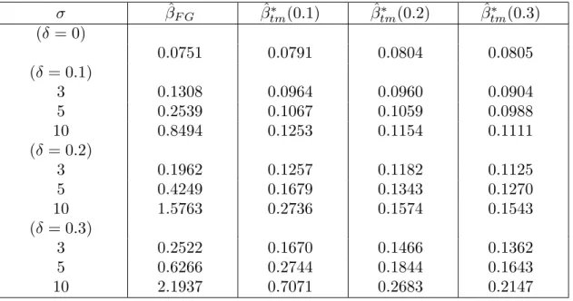
(17) 11. total of 10000 replications were performed and we compute the mean squares errors for the feasible generalized LSE βˆF G and feasible generalized trimmed mean βˆ∗ for tm. α1 = 1 − α2 = α = 0.1, 0.2, 0.3 where the total mean squared error is the square of the Euclidean distance between the estimator and true regression parameter β. For covenience, we here after in this section re-denote the feasible generalized trimmed mean by βˆtm (α). The mean squares errors are listed in Tables 1 and 2. ∗ Table 1. MSE’s for βˆF G and βˆtm under contaminated normal distribution (n = 30). σ (δ = 0) (δ = 0.1) 3 5 10 (δ = 0.2) 3 5 10 (δ = 0.3) 3 5 10. βˆF G. ∗ (0.1) βˆtm. ∗ (0.2) βˆtm. ∗ (0.3) βˆtm. 0.2096. 0.2241. 0.2179. 0.2556. 0.3746 0.7326 2.3055. 0.2874 0.3644 0.5463. 0.2697 0.3075 0.4184. 0.2698 0.2964 0.3714. 0.5543 1.2306 4.4579. 0.3963 0.5819 1.4236. 0.3600 0.4530 0.7820. 0.3300 0.4229 0.6012. 0.7075 1.7109 6.5214. 0.5380 0.9723 2.8921. 0.4448 0.6503 1.5105. 0.4101 0.5749 1.0893. ∗ Table 2. MSE’s for βˆF G and βˆtm under contaminated normal distribution (n = 100). σ (δ = 0) (δ = 0.1) 3 5 10 (δ = 0.2) 3 5 10 (δ = 0.3) 3 5 10. βˆF G. ∗ βˆtm (0.1). ∗ βˆtm (0.2). ∗ βˆtm (0.3). 0.0751. 0.0791. 0.0804. 0.0805. 0.1308 0.2539 0.8494. 0.0964 0.1067 0.1253. 0.0960 0.1059 0.1154. 0.0904 0.0988 0.1111. 0.1962 0.4249 1.5763. 0.1257 0.1679 0.2736. 0.1182 0.1343 0.1574. 0.1125 0.1270 0.1543. 0.2522 0.6266 2.1937. 0.1670 0.2744 0.7071. 0.1466 0.1844 0.2683. 0.1362 0.1643 0.2147.

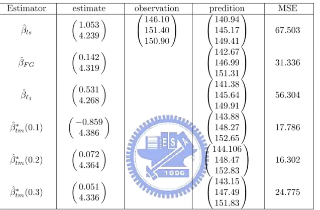
(18) 12. We have several conclusions drawn from Tables 1 and 2: (a) The MSE’s of these two estimators both increase when the contaminated percentage δ increases or contaminated variance σ 2 increases. This verifies the performance of the usual estimators, robust or non-robust. (b) The feasible generalized trimmed mean is relatively more efficient than the feasible generalized LSE in all cases of contaminated errors. This result shows that the feasible generalized trimmed mean is indeed, among the class of linear trimmed means, a robust one. In the next, we consider real data regression analysis. Many firms use past sales to forecast future sales. Suppose a wholesale distributor of sporting goods is interested in forecasting its sales revenue for each of the next 5 years. Since an inaccurate forecast may have dire consequences to the distributor, efficiency of the estimation of regression parameters is an important indicator in accuracy of forecasting. A data of a firm’s yearly sales revenue (thousands of dallars) with sample size n = 35 has been analyzed by Mendenhall and Sincich (1993). Since the scatter plot of the data revealed a linearly increasing trend, so a simple linear regression model yi = β0 + β1 xi + ²i , i = 1, ..., 35 seems to be reasonable to describe the trend. They first analyzed it with the least squares method that yields R2 = 0.98 which indicates that it is appropriate to be formulated as a linear regression model. They further displayed a plot of the residuals that revealed the existence of AR(1) errors and then the Durbin and Watson test has been performed that reject the hypothesis of null hypothesis ρ = 0. He also computed the prediction 95% confidence intervals for yearly revenues for years, 36-40, however, the interval estimates are wide that makes us less certain for the prediction of future observations (see this point in Mendenhall and Sincich (1993, p481)). We expect to have better analysis, based on the feasible generalized trimmed mean, in some sense. We follow their idea in evaluating the predition of the yearly revenues for years 36-40. Since the observations of these are available, we may compute the following mean square errors (MSE), 35 1 X MSE = (yi − (βˆ0 + βˆ1 xi ))2 3 i=33.

(19) 13. µ. ¶ µ ¶ β0 βˆ0 where ˆ is the estimate of corresponding the estimator. For this example, β1 β1 estimators considered include LSE βˆls , feasible generalized LSE βˆF G , `1 -norm estimator βˆ` and feasible generalized trimmed mean βˆtm (α) and their evaluated MSE’s are 1. listed in Table 3. Table 3. MSE’s for predictors based on some estimators Estimator βˆls. estimate µ ¶ 1.053 4.239 µ. βˆF G µ βˆ`1 µ ∗ βˆtm (0.1). 0.531 4.268. ¶. ¶. −0.859 4.386. µ ∗ βˆtm (0.2). µ ∗ βˆtm (0.3). 0.142 4.319. 0.072 4.364 0.051 4.336. ¶. ¶. ¶. observation   146.10  151.40  150.90. predition 140.94  145.17   149.41  142.67  146.99   151.31  141.38  145.64   149.91  143.88  148.27   152.65  144.106  148.47   152.83  143.15  147.49  151.83. MSE 67.503. 31.336. 56.304. 17.786. 16.302. 24.775. Surprisingly the feasible generalized trimmed means for several symmetric trimming proportions are with MSE’s all smaller than those of the other three estimators. The feasible generalized trimmed mean not only has asymptotic optimal properties in the class of linear trimmed means but also shows an interesting fact in prediction of future observations. 6. Appendix Let ² have distribution function F with probability density function f . Let zij represents the jth element of vector zi . The following conditions are similar to the standard ones for linear regression models as given in Ruppert and Carroll (1980) and Koenker and Portnoy (1987): Pn 4 (a3) n−1 i=1 zij = O(1),.

(20) 14. (a4) n−1 Z 0 Z = Qz + o(1), n−1 H00 Z = Qhz + o(1) and n−1 H00 H0 = Qh + o(1) where Qz and Qh are positive definite matrices and Qhz is a full rank matrix. Pn (a5) n−1 i=1 hi = θh + o(1), where θh is a finite vector. (a6) The probability density function and its derivative are both bounded and bounded away from 0 in a neighborhood of F −1 (α) for α ∈ (0, 1). Proof of Theorem 3.1. From condition (a2) and (A.10) of Ruppert and Carroll (1980), HH00 An Zβ = β + op (n−1/2 ). Inserting (2.4) in equation (2.7), we have n1/2 (βˆlt − β) = n1/2 HH00 Ae. (6.1). where we replace (1−ρ2 )1/2 ²1 by e1 that have the same asymptotic representation. Now Pn we develop a representation of n−1/2 H00 Ae. Let Uj (α, Tn ) = n−1/2 i=1 hij ei I(ei < F −1 (α) + n−1/2 zi0 Tn ) and U (α, Tn ) = (U1 (α, Tn ), ..., Up (α, Tn )). Also, let Tn∗ (α) = ˆ n1/2 [β(α) − β(α)]. Then n−1/2 H 0 An e = U (α2 , T ∗ (α2 )) − U (α1 , T ∗ (α1 )). From Jureckn. 0. n. ova and Sen’s (1987) extension of Billingsley’s Theorem (see also Koul (1992)), we have |Uj (α, Tn ) − Uj (α, 0) − n. −1. F. −1. (α)f (F. −1. (α)). n X. hij zi0 Tn | = op (1). (6.2). i=1. for j = 1, ..., p and Tn = Op (1). We know that, from Lai et al. (2004), −1 ˆ (F −1 (α))n−1/2 n1/2 (β(α) − β(α)) = Q−1 z f. n X. zi (α − I(ei ≤ F −1 (α))) + op (1). (6.3). i=1. From (6.2) and (6.3) n. −1/2. H00 An e. =n. −1/2. n X. hi ei I(F −1 (α1 ) ≤ ei ≤ F −1 (α2 )). i=1. +F. −1. −1/2 (α2 )Qhz Q−1 z n. −1/2 + F −1 (α1 )Qhz Q−1 z n. n X i=1 n X. zi (α2 − I(ei ≤ F −1 (α2 )) zi (α1 − I(ei ≤ F −1 (α1 )).. (6.4). i=1. Then the theorem is follwoed from (6.1) and (6.4). The proof of Theorem 3.5 is analogous as it for the above and then is skipped. Proof of Lemma 3.3. Denote by plim(Bn ) = B if Bn converges to B in probability. Let C = HH00 − (Z 0 An Z)−1 Z 0 ..

(21) 15. With this, plim(CZ) = plim(HH00 Z) − plim(Z 0 An Z)−1 Z 0 Z = 0. Then ˜ hH ˜ 0 = plim(HH00 (HH00 )0 ) HQ = plim((C + (Z 0 An Z)−1 Z 0 )(C + (Z 0 An Z)−1 Z 0 )0 ) = plim(CC 0 ) + plim((Z 0 An Z)−1 Z 0 Z(Z 0 An Z)−1 ) = plim(CC 0 ) + (α2 − α1 )−2 plim(Z 0 Z)−1 ≥ (α2 − α1 )−2 Q−1 z . Proof of Theorem 4.2. We here sketch only briefly a proof of the theorem. For detail references, see Chen et al. (2001) and Lai et al. (2003). With the fact that n1/2 (ˆ ρ − ρ) = Op (1) and condition (a1), we may see that ∗ ˆ + op (1). n1/2 (βˆltm − β) = n1/2 HH00 Ae. By letting M (t1 , t2 , α) = n−1/2. Pn i=1. (6.5). hi ei I(ei − n−1/2 t1 ²i−1 ≤ F −1 (α) + n−1/2 (zi +. n−1/2 t1 xi−1 )0 t2 + n−1/2 t1 F −1 (α)), we see that n−1/2 Zˆ 0 An e = M (T1∗ (α2 ), T2∗ , α2 ) − M (T1∗ (α1 ), T2∗ , α1 ). (6.5). ρ − ρ). However, using the same with T1∗ (α) = n1/2 (βˆ∗ (α) − β(α)) and T2∗ = n1/2 (ˆ methods in the proof of Lemma 3.5, we can see that M (T1 , T2 , α) − M (0, 0, α) = F. −1. (α)f (F. −1. −1/2. (α))n. n X. hi (zi0 T2 − T1 F −1 (α)) + op (1). i=1. (7.6). for any sequences T1 = Op (1) and T2 = Op (1). Then, from (6.5) and (6.6), we see that n−1/2 H 0 Aˆn e has the same representation of (6.4). Then (a1) and (6.5) further implies 0. the theorem.. ¤. References Aitken, A. C. (1935). On least squares and linear combination of observations. Proceedings of the Royal Society of Edinburg. 55, 42-48. Bai, Z.-D. and He, X. (1999). Asymptotic distributions of the maximal depth estimators for regression and multivariate location. The Annals of Statistics. 27, 1616-1637..

(22) 16. Chen, L.-A. (1997). An efficient class of weighted trimmed means for linear regression models. Statistica Sinica 7, 669-686. Chen, L-A, Welsh, A. H. and Chan, W. (2001) Linear winsorized means for the linear regression model. Statistica Sinica. 11, 147-172. Cochrane, D. and Orcutt, G. H. (1949). Application of least squares regressions to relationships containing autocorrelated error terms. Journal of the American Statistical Association, 44, 32-61. De Jongh, P. J. and De Wet, T. (1985), Trimmed Mean and Bounded Influence Estimators for the Parameters of the AR(1) Process, Communications in Statistics Theory and Methods, 14, 1361-1357. De Jongh, P. J., De Wet, T. and Welsch, A. H. (1988), Mallows-Type BoundedInfluence-Regression Trimmed Means, Journal of the American Statistical Association, 83, 805-810. Fomby, T. B., Hill, R. C. and Johnson, S. R. (1984). Advanced Econometric Methods. New York: Springer-Verlag. Giltinan, D. M., Carroll, R. J. and Ruppert, D. (1986), Some New Estimation Methods for Weighted Regression When There Are Possible Outliers, Technometrics, 28, 219-230. Huber, P. J. (1981). Robust Statistics. New York: Wiley. Jureˇ ckov´ a, J. (1977). Asymptotic relations of M -estimates and R-estimates in linear regression model. Annals of Statistics 5, 464-472. Jureckova, J. and Sen, P. K. (1987). An extension of Billingsley’s theorem to higher dimension M-processes. Kybernetica 23, 382-387. Koenker, R. W. and Bassett, G. W. (1978), Regression Quantiles, Econometrica 46, 33-50. Koenker, R. and Portnoy, S. (1990). M estimation of multivariate regression. Journal of the American Statistical Association, 85, 1060-1068. Koul, H.L. (1992). Weighted Empiricals and Linear Models. IMS Lecture Notes 21. Krasker, W. S. (1985), Two Stage Bounded-Influence Estimators for Simultaneous Equations Models, Journal of Business and Economic Statistics 4, 432-444..

(23) 17. Krasker, W. S. and Welsch, R. E. (1982), Efficient Bounded Influence Regression Estimation, Journal of the American Statistical Association 77, 595-604. Lai, Y.-H., Thompson, P. and Chen, L.-A. (2003). Generalized and Pseudo Generalized Trimmed Means for the Linear Regression with AR(1) Error Model. Statistics and Probability Letter, 67, 203-211. Mendenhall, W. and Sincich, T. (1993). A Second Course in Business Statistics: Regression Analysis. New York: Macmillan Publishing Company. Ruppert, D. and Carroll, R. J. (1980). Trimmed least squares estimation in the linear model. Journal of the American Statistical Association 75, 828-838. Serfling, R. J. (1980). Approximation Theorems of Mathematical Statistics. Wiley, New York. Welsh, A. H. (1987). The trimmed mean in the linear model. Annals of Statistics 15, 20-36..

(24)