國
立
交
通
大
學
統計學研究所
碩
士
論
文
家族性病例對照資料之統計分析
Statistical Analysis for Familial Case-Control Data
研 究 生:蘇筱嵐
指導教授:王維菁 博士
家族性病例對照資料之統計分析
Statistical Analysis for Familial Case-Control Data
研 究 生:蘇筱嵐 Student:Hsiao-Lan Su
指導教授:王維菁 博士 Advisor:Dr. Weijing Wang
國 立 交 通 大 學
統 計 學 研 究 所
碩 士 論 文
A Thesis
Submitted to Institute of Statistics
College of Science
National Chiao Tung University
in Partial Fulfillment of the Requirements
for the Degree of
Master
in
Statistics June 2010
Hsinchu, Taiwan, Republic of China
家族性病例對照資料之統計分析
學生:蘇筱嵐 指導教授:王維菁 博士
國立交通大學統計學研究所
摘
要
家族性病例對照資料研究方法近年來常使用於探討疾病與致病因子之
關係。本論文回顧了分析家族資料的統計文獻方法:針對得病與否的反應
變數,考慮了邏輯斯迴歸模型; 針對得病時間的反應變數,考慮了 Cox 等
比風險模型。我們討論如何將建立在個別性資料上之研究方法推廣至家族
性資料,並探討如何將適用於前瞻性資料的方法修改為分析病例對照資料
所需做的假設與調整。此外,我們也透過模擬實驗來驗證推論過程中所需
要之條件與比較參數估計之表現。
關鍵字:家族性病例對照資料研究;前瞻性研究;邏輯斯迴歸模型;Cox PH
模型;Clayton 模型
Statistical Analysis for Familial Case-Control Data
Student: Hsiao-Lan Su
Advisor: Dr. Weijing Wang
Institute of Statistics
National Chiao Tung University
Hsinchu, Taiwan
Abstract
Familial case-control data are frequently used to study the relationship between disease
and risk factors. In the thesis, we review literature for analyzing familial data. The logistic
model is applied to model the probability of disease incidence. The Cox proportional hazards
model is applied to model the age at onset of the disease. For each model, we discuss how to
extend the method and model developed for individual data to familial data. In addition, we
discuss the criteria and modification from prospective data to case-control data. We also
propose simulation algorithms for generating case-control data and then, based on simulated
data, examine parameter estimates and crucial properties of the inference procedure.
Keywords: Familial case-control study; Prospective study; Logistic regression; Cox PH model;
誌
謝
碩士生涯的終點,也代表了十八年學生旅程的結束。這兩年能有所成果,
首先必須感謝我的指導老師─王維菁教授,我在理論的推導與邏輯思考
上,一直不是很敏感,反應也很慢,是老師像母親般不厭其煩的引導我從
大方向思考,也讓我學會了該如何去統整概念和如何論述的技巧,更幫助
我撐起整篇論文的架構,老師給予的訓練在我往後的人生中將會受用無窮。
再來要感謝所有交大統研 97 與悶騷的研究室同學們,因為有你們的一同
努力與分享,學習之路不至於乏味而無援。還有高中與大學的好友們,你
們的支持與鼓勵是我向前邁進的動力。
也必須感謝交大統計所所有的老師與郭姐,給予了我們良好的學習環
境,讓我在碩士這兩年學到了許多知識。還有我的口試委員徐南蓉教授、
黃信誠教授與洪慧念教授,謝謝你們的協助與討論,使論文更加完善。
最後,我要感謝我的母親,我知道我不是個貼心的好女兒,這幾年來讓
您辛苦了,您無條件的支持使我求學過程中完全無後顧之憂。最後,我想
將這篇論文獻給我們永遠懷念的父親,我會盡力達成您的期望。
感謝一路上曾幫助過我的貴人,希望大家未來的人生都順利而快樂。
蘇筱嵐 謹誌于
國立交通大學統計學研究所
中華民國九十九年六月
Contents
1 Introduction ... 1
1.1 Motivation ... 1
1.2 Outline ... 2
2 An Overview of Case-Control Designs ... 3
2.1 Conventional Case-Control Designs ... 3
2.2 Familial Case-Control Designs ... 3
2.3 The Issue of Matching in Case-Control Designs ... 4
3 Logistic Regression on Different Designs ... 5
3.1 Conventional Case-Control Designs ... 5
3.2 Familial Case-Control Designs ... 7
3.2.1 Likelihood analysis based on familial prospective data ... 8
3.2.2 Likelihood analysis based on familial case-control data ... 10
4 Simulations for Logistic Regression Analysis ... 12
4.1 Data Generation for Individual Data ... 12
4.1.1 Prospective data of the true population ... 12
4.1.2 Case-control data from the true population ... 12
4.2 Analysis on Individual Data ... 13
4.3 Data Generation for Familial Data ... 15
4.3.1 Familial prospective data of the true population ... 15
4.3.2 Familial case-control data from the true population ... 15
4.4 Analysis on Familial Data ... 15
5 Regression Analysis Based on Familial Data ... 24
5.1 Likelihood Analysis Based on Probands ... 24
5.2 Likelihood Analysis Based on Familial data ... 27
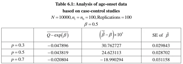
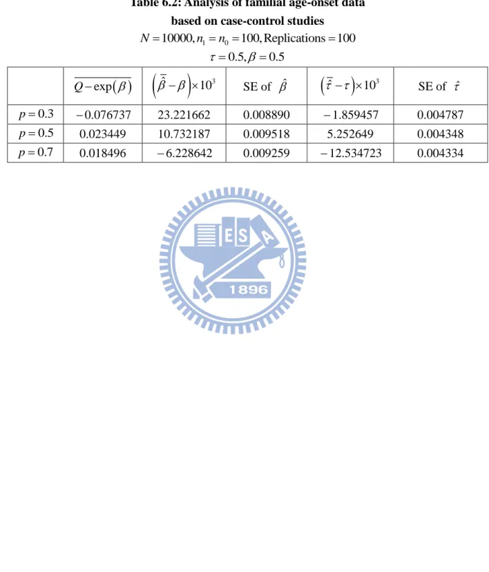
6 Simulations for Analysis of Age-onset Data from Case-Control Family Studies ... 33
6.1.1 Prospective data of the true population ... 33
6.1.2 Case-control data from the true population ... 34
6.2 Analysis on Individual Data ... 34
6.3 Data Generation for Familial Data ... 35
6.3.1 Familial prospective data of the true population ... 35
6.3.2 Familial case-control data from the true population ... 36
6.4 Analysis on Familial Data ... 36
7 Concluding Remarks ... 38
List of Tables
Table 3.1 Joint probability for
Y Y given p, r
Zp,Zr
... 10Table 4.1 Logistic regression analysis of case-control data ... 14
Table 4.2.A Checking reproducible properties of the population data (p=0.3) ... 17
Table 4.2.B Checking reproducible properties based on case-control data (p=0.3) ... 17
Table 4.2.C Checking reproducible properties based on case-control data (p=0.3) ... 18
Table 4.2.D Checking reproducible properties based on case-control data (p=0.3) ... 18
Table 4.3.A Checking reproducible properties of the population data (p=0.5) ... 19
Table 4.3.B Checking reproducible properties based on case-control data (p=0.5) ... 19
Table 4.3.C Checking reproducible properties based on case-control data (p=0.5) ... 20
Table 4.3.D Checking reproducible properties based on case-control data (p=0.5) ... 20
Table 4.4.A Checking reproducible properties of the population data (p=0.7) ... 21
Table 4.4.B Checking reproducible properties based on case-control data (p=0.7) ... 21
Table 4.4.C Checking reproducible properties based on case-control data (p=0.7) ... 22
Table 4.4.D Checking reproducible properties based on case-control data (p=0.7) ... 22
Table 4.5 The MLE of based on case-control familial data ... 23
Table 5.1 Age-matched case-control data ... 25
Table 5.2 Age-matched case-control familial data ... 28
Table 6.1 Analysis of age-onset data based on case-control studies ... 35
List of Figures
Chapter 1 Introduction
1.1 MotivationScientists are interested in studying the roles of genetic and environmental factors on the
development of a disease. Besides the information about whether the disease is present or not,
age-at-onset has been viewed as a useful quantitative trait for some commonly-seen complex
diseases. For example, early onset of breast cancer has been viewed as an important hallmark
for genetic predisposition. Figure 1 highlights the scientific background which motivates this
thesis. For a quantitative trait, statisticians can perform regression analysis which the effects
of the explanatory variables on the response.
Figure 1: Scientific Background
We focus on two quantitative traits, namely disease incidence and age-at-onset. Disease
incidence can be coded as a binary variable. Age-onset variables are continuous but may be
censored due to termination of the study or loss to follow-up. Genetic, environmental and
individual factors are treated as observed covariates. Their influences on the chosen response
variable are of major interest. If disease incidence is the response variable, logistic regression
models can be adopted. If age-at-onset is studied, failure-time regression models such as Cox
proportional hazards models can be applied. When genetic information is not directly Environmental factors Individual factors Quantitative Traits: Incidence Age-onset Others Genetic factors
measured, familial data can be used to detect its influence. Familial aggregation often
indicates that genetic or shared environmental factors play some role in the development of
the disease.
From the aspect of data design, the case-control sampling study is often applied to gather
the information of rare diseases. It has the advantage that sufficient number of cases can be
obtained and hence is cheaper and more convenient in comparison with a prospective study.
In recent years, familial case-control designs have become a popular choice in genetic
epidemiology. However statistical inference based on familial case-control data deserves
careful investigation since the underlying probability structure is not straightforward.
1.2 Outline
The purpose of the thesis is to review related literature under a unified framework and
examine some theoretical statements via simulations. In Chapter 2, we provide some
background for different types of case-control designs. In Chapter 3, we review literature on
logistic regression for familial prospective studies and case-control designs. Chapter 4
contains some simulation results which are conducted to verify crucial probability statements
for logistic regression analysis. In Chapter 5, we review literature on familial age-onset data
based on case-control designs. Chapter 6 contains simulation studies for checking the
assumptions that are required in analysis of age-onset data from case-control family studies.
Chapter 2 An Overview of Case-control Designs
Case-control designs are preferable because they are cheaper and more convenient. In
this chapter, we focus on two common case-control designs: namely the conventional and
familial designs.
2.1 Conventional Case-control Designs
Conventional case-control designs begin by recruiting a group of individuals with a specific
disease as “cases” and the other group of non-diseased individuals as “controls”. Cases and
controls are compared based on risk factors including familial history of the disease. Here
positive familial history is defined as presence of the disease in one or more first-degree
relatives. However potential bias may arise due to incorrect information of recall.
Furthermore individuals may differ in their family sizes so that positive family history is more
likely to occur in a larger family. The family sizes differ in cases and controls can lead to false
results. Liang (2000) discussed potential biases for conventional case-control designs in
details.
2.2 Familial Case-Control Designs
Familial data obtained from case-control designs are frequently used to detect disease
aggregation in families. This design begins by identifying a sample of diseased cases and an
independent sample of disease-free controls, and for each individual, hereafter called a
“proband”, determines his/her covariates, the family structure, and the disease status and covariates of relatives in the family. The disease status of relatives is treated as one part of the
responses in the model.
A major difference between the two designs lies in the sampling unit. The sampling unit in
familial case-control designs is a pre-defined set of family members. Compared to the
conventional design, familial case-control designs provide direct evaluations of the relatives
and can avoid misclassification of family history. It is also useful for genetic counseling.
2.3 The Issue of Matching in Case-Control Designs
In case-control designs, there are some confounding variables that may affect the
evaluation of the association between disease incidence and risk factors. So, sometimes we
must consider the necessity to match these confounding variables in the design stage. The
purpose of matching is to let the units between cases and controls have more comparability.
The matching method includes frequency matching and individual matching. In
conventional case-control design, if individual matching is part of the design, the conditional
logistic regression method mentioned in Breslow and Day (1980) may be adopted. When in a
familial case-control design, we note that the sampling units are families. So the matching
between case probands and control probands doesn’t guarantee the matching between case
relatives and control relatives. Thus the matching procedure in such studies should be subject
to some modification. First, the matching in design stage must be run under the condition that
the confounding variables are familial, for example: races. Second, correlations among
relatives have to be dealt with. Liang (1987) proposed a method for analyzing the matched
designs which accounts for the within-family correlation. For age-onset responses, Li et al.
(1998) also discussed situations under familial structure and matched procedure.
Finally, Sturmer and Brenner (2000) discussed the issue of the balance between power
Chapter 3 Logistic Regression on Different Designs
Logistic regression models are commonly adopted for modeling the relationship between
a binary response and covariates. We first discuss statistical inference based on prospective
studies which can be easily understood. Then we discuss how to construct the likelihood
function if the sample is obtained from a case-control design. Finally we will review the
literature on logistic regression analysis for familial case-control studies.
Denote Y as a binary indicator for disease status. Specifically Y 1 represents that the individual is diseased while Y 0 indicates that the individual is free of the disease. Denote
Z as a p1 vector of covariates. Consider the following logistic regression model:
exp( ) Pr( 1| ) 1 exp( ) T T Z Y Z Z . (3.1)
Let {( ,Y Zi i) (i1,..., )}n denote the observed sample. If the data are collected from a
prospective design, the likelihood function can be written as
1 1 exp( ) 1 1 exp( ) 1 exp( ) i i Y Y T n i T T i i i Z Z Z
. (3.2)A case-control study, by contrast, identify a sample of diseased cases: Y 1 and another independent sample of non-diseased controls: Y 0 . The covariate Z is measured
afterwards. Notice that the distribution of data from a case-control study is based on
Pr Z Y instead of | Pr
Y Z as given in (3.1). However logistic regression analysis can |
still be applied to both sampling designs (Prentice and Pyke, 1979). In Sections 3.1 and 3.2,we will review the results of Whittemore (1995) in which the probability structure under
conventional and familial case-control designs is well examined.
3.1 Conventional Case-Control Designs
Let be the target population. The logistic regression model in (3.1) is equivalent to
Pr( 1| , ) log Pr( 0 | , ) T Y Z Z Y Z (3.3)
where is the intercept that represents the log odds for developing the disease of the baseline group, and is the log odds ratio between a subject with covariate Z and a subject of the baseline group. Since reflects the effect of Z on Y , it is the parameter of
major interest.
As mention earlier, a sample based on a case-control design involves Pr
Z Y| ,
. Applying Baye’s rule, we obtainPr( | 1, ) Pr( 0 | ) exp( ) exp( ). Pr( | 0, ) Pr( 1| ) T Z Y Y Z Z Y Y (3.4a)
Whittemore (1995) mentioned that one can imagine a hypothetical population denoted as * in which the covariate distribution is the same as in such that
* * Pr( | 1, ) Pr( | 1, ) Pr( 0 | ) exp( ) exp( ) Pr( | 0, ) Pr( | 0, ) Pr( 1| ) T Z Y Z Y Y Z Z Y Z Y Y . (3.4b) Define * * Pr( 0 | ) Pr( 1| ) exp( ) exp( ) Pr( 1| ) Pr( 0 | ) Y Y Y Y .
One can rewrite (3.4b) as
* * * * Pr( | 1, ) Pr( 0 | ) exp( ) exp( ) Pr( | 0, ) Pr( 1| ) T Z Y Y Z Z Y Y . (3.5)
From (3.5), we can construct the following logistic model based on *:
* * Pr( 1| , ) log Pr( 0 | , ) T Y Z Z Y Z . (3.6)
Now we discuss the implication of the above analysis. Comparing the two models in (3.3)
and (3.6), they differ in the intercept parameter but have the same slope parameter, which is of
major interest. In a case-control design, the sampling distribution is based on
*
Pr Z Y| 1, and Pr
Z Y| 0, *
, where
*
*
*
* Pr | Pr | 1, Pr 1| , Pr 1| Z Z Y Y Z Y ;
*
*
*
* Pr | Pr | 0, Pr 0 | , Pr 0 | Z Z Y Y Z Y . Notice that
* * Pr | Pr | Z Y is independent with parameters. The likelihood function for
case-control data can be constructed based on model (3.6). Accordingly case-control data can
be treated as prospective data from * if the following condition holds:
* * Pr( | 1, ) Pr( | 1, ) Pr( | 0, ) Pr( | 0, ) Z Y Z Y Z Y Z Y . (3.7)
As long as (3.7) is satisfied in collecting the case-control sample, one can proceed the
regression analysis, by pretending that the sample is from a prospective study, to obtain an
estimate of which is still reliable. We will examine the crucial condition in (3.7) via simulations.
3.2 Familial Case-Control Designs
In analysis of familial data, some studies ignored probands’ information and only focus
on relatives’ data. Such an approach may lose efficiency by ignoring useful information in
probands’ data. Whittemore (1995) applied multivariate techniques to analyze familial
case-control data. Specifically she proposed a two-stage sampling procedure. Specifically in
the first stage, two types of probands (case and control) are sampled and then, in the second
stage, their relatives are sampled. To simplify the discussion, we focus on bivariate analysis
which means that only one relative is sampled based on each proband. The resulting
likelihood analysis contains two components. One involves the logistic model on probands as
introduced earlier. The other component is related to the model which measures the
dependence between a proband and his/her relatives.
Let (Y Zp, p) and ( ,Y Zr r) be the disease status and covariates for a proband and his/her
relative respectively. Denote Y (Y Yp, r) and Z (Zp,Zr). We will first discuss likelihood
design.
3.2.1 Likelihood analysis based on familial prospective data
A prospective study involves sampling from
Pr( ,Y Zr|Zp)Pr( | ) Pr(Y Z Zr|Zp). (3.8)
When only one relative is involved, Pr( | )Y Z Pr(Yp y Yp, r yr|Z Zp, r) for y* 0,1 and
* = ,p r . Note that
Pr( | )Y Z =Pr(Yp|Z Zp, r) Pr(Y Y Zr| p, ).
Whittemore (1995) mentioned that a reasonable joint model should satisfy the so-called
“reproducible” assumption such that
1 0 Pr( , | , ) r r y p p r r p r y Y y Y y Z Z
Pr(Yp yp|Zp); (3.9a) 1 0 Pr( , | , ) p p y p p r r p r y Y y Y y Z Z
Pr(Yr yr|Zr). (3.9b)That is, the covariate of a person is sufficient to determine his/her disease status and hence the
relative’s covariate does not contribute extra information. The paper examines the plausibility
of the reproducible assumption. Suppose that the dependence between Yp and Y within the r
same family may also be attributed to some un-measured latent variable denoted as U . If Pr(U Z| )Pr( )U , the reproducible assumption can be achieved. Whether this assumption makes sense depends on the scientific problem at hand.
When (3.9a) is true, it follows that
Pr( | )Y Z =Pr(Yp|Zp) Pr(Y Y Zr | p, ). (3.10)
log Pr( 1| ) Pr( 0 | ) p p T p p p Y Z Z Y Z .
The second quantity Pr(Y Y Zr | p, )Pr(Y Y Zr | p, p,Zr) in (3.10) involves the dependence between a proband and his/her relative which is of major interest. Denote observed data
as{(Y Y Zpi, ri, pi,Zri) (i1,..., )}n . If the data is collected from a prospective sampling design,
the likelihood function can be written as
1 , , Pr , , | i i i i n p r r p i L Y Y Z Z
1 1 Pr | Pr | , i i i i n n p p r p i i i Y Z Y Y Z
(1) (2) , , , L L , (3.11)where L(1)
,
has the form as in (3.2) and denotes additional parameter inPr(Y Y Zr | p, ) . Additional joint model assumption is required to specify the form of
Pr(Y Y Zr | p, ).
One model choice is the following model first proposed by Bahadur (1961):
1 1 Pr(( , ) | ( , )) ( ) (1yp ) yp( ) (1yr ) yr(1 ) p r p r p p r r p r Y Y Z Z p p p p t t (3.12) where
* * * * * * , 1 y p t p r p p , and * * * * * exp( ) Pr( 1| ) * , 1 exp( ) T T Z p Y Z p r Z .The coefficient satisfies the following constraint:
1 1 1 1 min , min , . 1 1 1 1 p r r p p r p r p r r p p r p r p p p p p p p p p p p p p p p p We will check whether this model satisfies the reproducible assumption via simulations. The
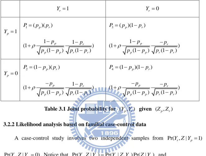
following table summarizes the joint probability of (Yp,Yr) given (Zp,Zr).
1 r Y Yr 0 1 p Y 1 ( p)( r) P p p 1 1 (1 ) (1 ) (1 ) p r p p r r p p p p p p 3 ( p)(1 r) P p p 1 (1 ) (1 ) (1 ) p r p p r r p p p p p p 0 p Y 2 (1 p)( r) P p p 1 (1 ) (1 ) (1 ) p r p p r r p p p p p p 4 (1 p)(1 r) P p p (1 ) (1 ) (1 ) p r p p r r p p p p p p
Table 3.1 Joint probability for (Y Yp, r) given (Zp,Zr)
3.2.2 Likelihood analysis based on familial case-control data
A case-control study involves two independent samples from Pr( ,Y Z Yr | p 1) and
Pr( ,Y Z Yr | p 0). Notice that Pr( ,Y Z Yr | p)Pr(Y Z Yr | , p) Pr( |Z Yp) and
Pr( |Z Yp)Pr(Z Z Yp, r | p)Pr(Zp|Yp) Pr(Z Y Zr | p, p).
The reproducible assumption implies that, given Zp, Yp and Z are independent. Hence r
Pr( |Z Yp)Pr(Zp |Yp) Pr(Zr|Zp). In summary we have
Pr Y Z Yr, | p Pr Y Z Yr, | p Pr Zp|Yp Pr Zr|Zp
Pr(Zp|Yp)
Pr(Y Z Yr| , p) Pr(Zr |Zp)
. (3.13)
Recall that Pr(Zp|Yp) can be analyzed assuming that the data is from a prospective sample
* * Pr( 1| , ) log Pr( 0 | , ) p p T p p p Y Z Z Y Z .
Accordingly the retrospective likelihood function is given by
* 1 , , , Pr , | i i n r i p i L Y Z Y
1 1 Pr | Pr | , i i i i n n p p r p i i i Z Y Y Y Z
*(1) (2) , , , L L .Notice that the information of is also contained in familial case-control data when the reproducible assumption holds for the joint model.
Chapter 4 Simulations for Logistic Regression Analysis
In this chapter, we propose data generation algorithms to simulate case-control data for
logistic regression analysis. Some crucial probability statements will be examined to verify
whether the simulated data are reliable for statistical inference.
4.1 Data Generation for Individual Data 4.1.1 Prospective data of the true population
First of all, we generate population data from the model:
exp
Pr 1| , 1 exp Z Y Z Z .Then set the values of the parameters: , and p. The algorithm is summarized below: Step 1: Generate Zi Bernoulli( )p
Step 2: Given Z , generate i
exp Bernoulli . 1 exp i i i Z Y Z The procedure is repeated for i1,...,N for very large N , say N10000. Denote
{( ,Y Zi i)(i 1,...,N)}
.
4.1.2 Case-control data from the true population
Suppose that we generate nN observations from the population with n persons 1
from the case group with Y 1 and n0 n n1 persons from the control group Y 0. The procedure is stated as follows.
Step 1: Randomly select n subjects from the case group and record their values of 1 Zi;
Step 2: Randomly select n subjects from the control group and record their values of 0
i
We briefly discuss how to implement Step 1 since Step 2 follows a similar procedure. First
identify the case population: 1 {(Yi 1,Zi) (i1,...,N1)}where 1
1 ( 1) N i i N I Y
. Theobjective is to select n observations from 1 N subjects. Label the subjects in 1 1 from 1 to
1
N . At the first time, generate U U
0,1 and define s
N1U
, where
is the Gauss function. A subject with label “s ” is selected into the case-control sample and removedfrom 1. The procedure is repeated n times. Specifically at the 1 kth time, generate
0,1U U and a subject with a re-defined label s
(N1 k 1) U
is selected from the remaining case population containing N1 k 1 subjects. Finally the case sample is formed and denoted as {(Yk 1,Zk) (k 1,..., )}n1 . The control sample can be generated in a similar way.4.2. Analysis on Individual Data
We examine whether the proposed case-control sampling procedure produces reliable
data. We let 1 1 * 1 1 ( *, 1) / ( 1) ( *, 0) / ( 0) N N i i i i i N N i i i i i I Z Y I Y R I Z Y I Y
*0,1
and
1 1 * 1 1 *, 1 / *, 0 / n i i i n i i i I Z Y n r I Z Y n
* 0 , 1
be the empirical estimates of
Pr * | 1, Pr * | 0, Z Y Z Y and
* * Pr * | 1, Pr * | 0, Z Y Z Y respectively.The first criteria to evaluate the quality of data is checking whether r is close to * R . The *
the combined case-control data: {(Yk 1,Zk) (k 1,..., )}n1 and {(Yk 0,Zk) (k 1,...,n0)}. The MLE of ˆ and ˆ are obtained. By checking whether ˆ is close to the true value, we can examine whether the case-control data provide reliable information of . The results are summarized in Tables 4.1. We observe that the empirical estimate r is close to * R *
obtained from the population data, the estimations of ˆ are also stable and close to the true value.
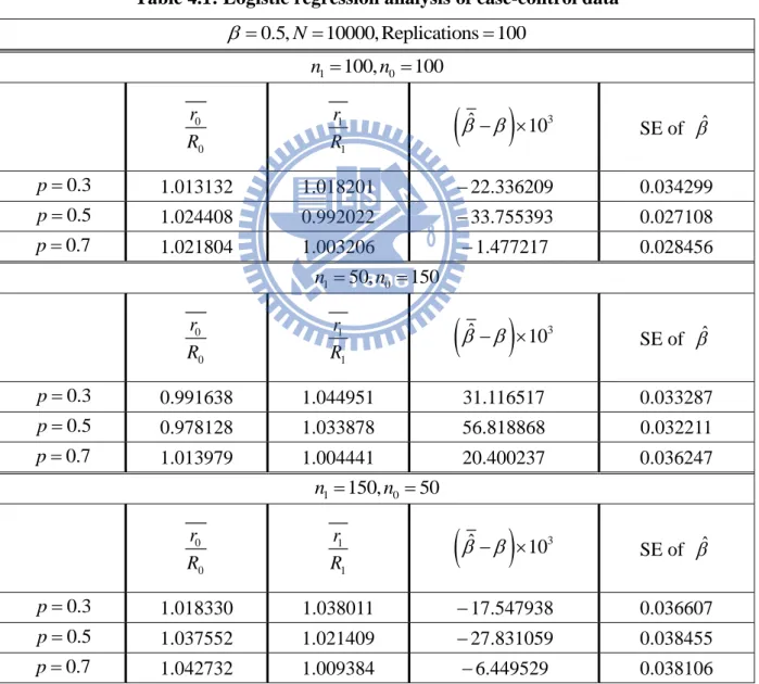
Table 4.1: Logistic regression analysis of case-control data
0.5,N 10000, Replications 100 1 100, 0 100 n n 0 0 r R 1 1 r R
3 ˆ 10 SE of ˆ 0.3 p 1.013132 1.018201 22.336209 0.034299 0.5 p 1.024408 0.992022 33.755393 0.027108 0.7 p 1.021804 1.003206 1.477217 0.028456 1 50, 0 150 n n 0 0 r R 1 1 r R
3 ˆ 10 SE of ˆ 0.3 p 0.991638 1.044951 31.116517 0.033287 0.5 p 0.978128 1.033878 56.818868 0.032211 0.7 p 1.013979 1.004441 20.400237 0.036247 1 150, 0 50 n n 0 0 r R 1 1 r R
3 ˆ 10 SE of ˆ 0.3 p 1.018330 1.038011 17.547938 0.036607 0.5 p 1.037552 1.021409 27.831059 0.038455 0.7 p 1.042732 1.009384 6.449529 0.0381064.3 Data Generation for Familial Data
4.3.1 Familial prospective data of the true population
We first generate data following the model proposed by Bahadur (1961). First set the
values of the parameters: , , and p. The algorithm is summarized below: Step 1: Generate
i p
Z following Bernoulli
p andi r
Z independently also following
Bernoulli
p ; Step 2: Given i p Z and i rZ , compute P P P P mentioned in Table 3.1; 1, 2, 3, 4 Step 3: Generate Ui Uniform 0,1
; Step 4: Set 1 1 1 2 1 2 1 2 3 1 2 3 1, 1 if 0 0, 1 if 1, 0 if 0, 0 if 1 i i i i i i i i p r i p r i p r i p r i Y Y U P Y Y P U P P Y Y P P U P P P Y Y P P P U .
The procedure is repeated for i1,...,N for N10000.
4.3.2 Familial case-control data from the true population
The procedure is stated as follows.
Step 1: Randomly select n probands from the case families with 1 Ypi 1 and record the
values of ( , , )
i i i
p r r
Z Y Z ;
Step 2: Randomly select n probands from the control families with 0 Ypi 0 and record
their values of ( , , )
i i i
p r r
Z Y Z .
4.4. Analysis on Familial Data
We first examine whether the algorithm for generating perspective data satisfies the
1 1 1 ( , , ) ( , , ) ( , ) N pi p pi p ri r i p p r N pi p ri r i I Y y Z z Z z q y z z I Z z Z z
, and 1 1 1 ( , ) ( , ) ( ) N pi p pi p i p p N pi p i I Y y Z z q y z I Z z
; 1 2 1 ( , , ) ( , , ) ( , ) N ri r pi p ri r i r p r N pi p ri r i I Y y Z z Z z q y z z I Z z Z z
, and 2( r, r) q y z 1 1 ( , ) ( ) N ri r ri r i N ri r i I Y y Z z I Z z
.The reproducible condition should imply that q y z1( p, p,zr) q y z1( p, p) and q y z2( r, p,zr) 2( r, r)
q y z
. The results of these quantities based on prospective data and case-control data from the true population are recorded in Table 4.2 ~ 4.4. In analyzing the case-control familial
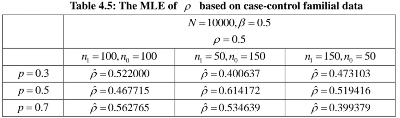
data, we assume and are known and then obtain the MLE of . By checking whether ˆ is close to the true value, we can examine whether the familial case-control data provide reliable information of the association in a family. This result is given in Table 4.5.
We observe that the performance of the reproducible properties is good in our population
data which means that the model is appropriate. But sometimes the reproducible properties do
not reflected in the simulated case-control data. Accordingly the estimations of ˆ will have worse results in these situations.
Table 4.2.A: Checking reproducible properties of the population data (p=0.3) 10000 N (y zp, p)(1,1) (y zp, p)(1, 0) (y zp, p)(0,1) (y zp, p)(0, 0) 1 r z q1 0.734649 q10.630283 q1 0.265351 q10.369717 0 r z q1 0.729743 q10.638770 q1 0.270257 q10.361230 1 q 0.731267 q10.636183 q1 0.268733 q10.363817 (y zr, r)(1,1) (y zr, r)(1, 0) (y zr, r)(0,1) (y zr, r)(0, 0) 1 p z q2 0.718202 q2 0.607213 q2 0.281798 q2 0.392787 0 p z q2 0.752438 q2 0.642232 q2 0.247562 q2 0.357768 2 q 0.742251 q2 0.632012 q2 0.257749 q2 0.367988
Table 4.2.B: Checking reproducible properties based on case-control data (p=0.3)
1 0 10000, 100, 100 N n n (y zp, p)(1,1) (y zp, p)(1, 0) (y zp, p)(0,1) (y zp, p)(0, 0) 1 r z q1 0.545455 q10.547170 q1 0.454545 q10.452830 0 r z q1 0.696970 q10.391304 q1 0.303030 q10.608696 1 q 0.636364 q10.448276 q1 0.363636 q10.551724 (y zr, r)(1,1) (y zr, r)(1, 0) (y zr, r)(0,1) (y zr, r)(0, 0) 1 p z q2 0.590909 q2 0.575758 q2 0.409091 q2 0.424242 0 p z q2 0.698113 q2 0.521739 q2 0.301887 q2 0.478261 2 q 0.666667 q2 0.536000 q2 0.333333 q2 0.464000
Table 4.2.C: Checking reproducible properties based on case-control data (p=0.3) 1 0 10000, 50, 150 N n n (y zp, p)(1,1) (y zp, p)(1, 0) (y zp, p)(0,1) (y zp, p)(0, 0) 1 r z q1 0.363636 q10.282609 q1 0.636364 q10.717391 0 r z q1 0.222222 q10.218750 q1 0.777778 q10.781250 1 q 0.275862 q10.239437 q1 0.724138 q10.760563 (y zr, r)(1,1) (y zr, r)(1, 0) (y zr, r)(0,1) (y zr, r)(0, 0) 1 p z q2 0.590909 q2 0.222222 q2 0.409091 q2 0.777778 0 p z q2 0.652174 q2 0.427083 q2 0.347826 q2 0.572917 2 q 0.632353 q2 0.371212 q2 0.367647 q2 0.628788
Table 4.2.D: Checking reproducible properties based on case-control data (p=0.3)
1 0 10000, 150, 50 N n n (y zp, p)(1,1) (y zp, p)(1, 0) (y zp, p)(0,1) (y zp, p)(0, 0) 1 r z q1 0.782609 q10.763158 q1 0.217391 q10.236842 0 r z q1 0.818182 q10.690476 q1 0.181818 q10.309524 1 q 0.807692 q1 0.713115 q1 0.192308 q10.286885 (y zr, r)(1,1) (y zr, r)(1, 0) (y zr, r)(0,1) (y zr, r)(0, 0) 1 p z q2 0.695652 q2 0.527273 q2 0.304348 q2 0.472727 0 p z q2 0.842105 q2 0.619048 q2 0.157895 q2 0.380952 q 0.786885 q 0.582734 q 0.213115 q 0.417266
Table 4.3.A: Checking reproducible properties of the population data (p=0.5) 10000 N (y zp, p)(1,1) (y zp, p)(1, 0) (y zp, p)(0,1) (y zp, p)(0, 0) 1 r z q1 0.725902 q10.611177 q1 0.274098 q10.388823 0 r z q1 0.739654 q10.627195 q1 0.260346 q10.372805 1 q 0.732735 q10.619038 q1 0.267265 q10.380962 (y zr, r)(1,1) (y zr, r)(1, 0) (y zr, r)(0,1) (y zr, r)(0, 0) 1 p z q2 0.729869 q2 0.611089 q2 0.270131 q2 0.388911 0 p z q2 0.726092 q2 0.616170 q2 0.273908 q2 0.383830 2 q 0.727973 q2 0.613609 q2 0.272027 q2 0.386391
Table 4.3.B: Checking reproducible properties based on case-control data (p=0.5)
1 0 10000, 100, 100 N n n (y zp, p)(1,1) (y zp, p)(1, 0) (y zp, p)(0,1) (y zp, p)(0, 0) 1 r z q1 0.500000 q10.390244 q1 0.500000 q10.609756 0 r z q1 0.548387 q10.529412 q1 0.451613 q10.470588 1 q 0.527778 q10.467391 q1 0.472222 q10.532609 (y zr, r)(1,1) (y zr, r)(1, 0) (y zr, r)(0,1) (y zr, r)(0, 0) 1 p z q2 0.695652 q2 0.532258 q2 0.304348 q2 0.467742 0 p z q2 0.609756 q2 0.470588 q2 0.390244 q2 0.529412 2 q 0.655172 q2 0.504425 q2 0.344828 q2 0.495575
Table 4.3.C: Checking reproducible properties based on case-control data (p=0.5) 1 0 10000, 50, 150 N n n (y zp, p)(1,1) (y zp, p)(1, 0) (y zp, p)(0,1) (y zp, p)(0, 0) 1 r z q1 0.325581 q10.245614 q1 0.674419 q10.754386 0 r z q1 0.306122 q10.137255 q1 0.693878 q10.862745 1 q 0.315217 q10.194444 q1 0.684783 q10.805556 (y zr, r)(1,1) (y zr, r)(1, 0) (y zr, r)(0,1) (y zr, r)(0, 0) 1 p z q2 0.604651 q2 0.244898 q2 0.395349 q2 0.755102 0 p z q2 0.614035 q2 0.215686 q2 0.385965 q2 0.784314 2 q 0.610000 q2 0.230000 q2 0.390000 q2 0.770000
Table 4.3.D: Checking reproducible properties based on case-control data (p=0.5)
1 0 10000, 150, 50 N n n (y zp, p)(1,1) (y zp, p)(1, 0) (y zp, p)(0,1) (y zp, p)(0, 0) 1 r z q1 0.825397 q10.636364 q1 0.174603 q10.363636 0 r z q1 0.733333 q10.787879 q1 0.266667 q10.212121 1 q 0.780488 q10.701299 q1 0.219512 q10.298701 (y zr, r)(1,1) (y zr, r)(1, 0) (y zr, r)(0,1) (y zr, r)(0, 0) 1 p z q2 0.777778 q2 0.550000 q2 0.222222 q2 0.450000 0 p z q2 0.727273 q2 0.727273 q2 0.272727 q2 0.272727 q 0.757009 q 0.612903 q 0.242991 q 0.387097
Table 4.4.A: Checking reproducible properties of the population data (p=0.7) 10000 N (y zp, p)(1,1) (y zp, p)(1, 0) (y zp, p)(0,1) (y zp, p)(0, 0) 1 r z q1 0.725744 q10.631256 q1 0.274256 q10.368744 0 r z q1 0.713138 q10.625140 q1 0.286862 q10.374860 1 q 0.721928 q10.629445 q1 0.278072 q10.370555 (y zr, r)(1,1) (y zr, r)(1, 0) (y zr, r)(0,1) (y zr, r)(0, 0) 1 p z q2 0.718154 q2 0.607750 q2 0.281846 q2 0.392250 0 p z q2 0.731822 q2 0.622896 q2 0.268178 q2 0.377104 2 q 0.722294 q2 0.612238 q2 0.277706 q2 0.387762
Table 4.4.B: Checking reproducible properties based on case-control data (p=0.7)
1 0 10000, 100, 100 N n n (y zp, p)(1,1) (y zp, p)(1, 0) (y zp, p)(0,1) (y zp, p)(0, 0) 1 r z q1 0.505155 q10.428571 q1 0.494845 q10.571429 0 r z q1 0.577778 q10.437500 q1 0.422222 q10.562500 1 q 0.528169 q10.431034 q1 0.471831 q10.568966 (y zr, r)(1,1) (y zr, r)(1, 0) (y zr, r)(0,1) (y zr, r)(0, 0) 1 p z q2 0.659794 q2 0.422222 q2 0.340206 q2 0.577778 0 p z q2 0.642857 q2 0.375000 q2 0.357143 q2 0.625000 2 q 0.654676 q2 0.409836 q2 0.345324 q2 0.590164
Table 4.4.C: Checking reproducible properties based on case-control data (p=0.7) 1 0 10000, 50, 150 N n n (y zp, p)(1,1) (y zp, p)(1, 0) (y zp, p)(0,1) (y zp, p)(0, 0) 1 r z q1 0.261364 q10.111111 q1 0.738636 q10.888889 0 r z q1 0.363636 q10.260870 q1 0.636364 q10.739130 1 q 0.295455 q10.161765 q1 0.704545 q10.838235 (y zr, r)(1,1) (y zr, r)(1, 0) (y zr, r)(0,1) (y zr, r)(0, 0) 1 p z q2 0.431818 q2 0.386364 q2 0.568182 q2 0.613636 0 p z q2 0.600000 q2 0.521739 q2 0.400000 q2 0.478261 2 q 0.488722 q2 0.432836 q2 0.511278 q2 0.567164
Table 4.4.D: Checking reproducible properties based on case-control data (p=0.7)
1 0 10000, 150, 50 N n n (y zp, p)(1,1) (y zp, p)(1, 0) (y zp, p)(0,1) (y zp, p)(0, 0) 1 r z q1 0.724490 q10.575758 q1 0.275510 q10.424242 0 r z q1 0.857143 q10.900000 q1 0.142857 q10.100000 1 q 0.768707 q1 0.698113 q1 0.231293 q10.301887 (y zr, r)(1,1) (y zr, r)(1, 0) (y zr, r)(0,1) (y zr, r)(0, 0) 1 p z q2 0.734694 q2 0.755102 q2 0.265306 q2 0.244898 0 p z q2 0.787879 q2 0.800000 q2 0.212121 q2 0.200000 q 0.748092 q 0.768116 q 0.251908 q 0.231884
Table 4.5: The MLE of based on case-control familial data 10000, 0.5 N 0.5 1 100, 0 100 n n n150,n0 150 n1 150,n0 50 0.3 p ˆ 0.522000 ˆ 0.400637 ˆ 0.473103 0.5 p ˆ 0.467715 ˆ 0.614172 ˆ 0.519416 0.7 p ˆ 0.562765 ˆ 0.534639 ˆ 0.399379
Chapter 5 Regression Analysis Based on Familial Data
For those who have developed the disease, the age at onset may be informative. As
mentioned in Li et al. (1998), early age of onset has been a hallmark for genetic predisposition
in most of diseases that aggregate in families. When age-at-onset is chosen as the primary
response, the effect of censoring has to be considered in the analysis.
In this chapter, we discuss several important issues on analyzing familial age-onset data.
Specifically denote T as the age-onset variable and Z as a p1 vector of covariates. The Cox proportional hazards model is the most well-known model for failure time variables
which can be written as
|
0
exp
,T
t Z t Z
(5.1) where 0( )t is the baseline hazard function and measures the effect of Z on the hazard and is of major interest. In familial failure-time analysis, the Cox model is imposed on
probands. For inference of , we first review the analysis based on a prospective sample and then extend the discussion to a valid case-control sample. Finally we will discuss the
modeling and inference frameworks when familial case-control data are collected.
5.1 Likelihood Analysis Based on Probands
Under right censoring, let C be the censoring variable. One observes that X T C,
( )
I T C
and covariates Z. In prospective studies, we identify a sample of individuals with specified covariates: Z and then determine their observed time and disease status: i
(Xi, )i for i1,...,n. At time t , the risk set can be denoted as R t( ){ :i Xi t i, 1,..., }n .
Given the risk set information, a subject failing at time t with covariate Zj given jR t( )
will contribute to the partial likelihood by
0 0 exp exp | . | exp exp T T j j j T T i i i t Z Z t Z t Z t Z Z
(5.2)Prentice and Breslow (1978) discussed the likelihood formulation based on case-control
age-onset data. It is important to first introduce the sampling procedure which involves how
to match a case subject with a control subject. Specifically at time t , m t observations are ( ) sampled from the case population containing those who develop the disease at time t and,
independently, n t( ) observations are sampled from the control population containing those
who have not developed the disease up to time t . Observed data can be summarized in Table
5.1.
Time:t i Case:
X ti, 1
Control:
X ti, 0
1 t m t individuals ( )1 n t individuals ( )1 i t m t individuals ( )i n t individuals ( )i k t m t( )k individuals n t( )k individuals
Table 5.1 Age-matched case-control data
The case-control design for collecting age-onset data considers sampling from the
conditional distribution of Z based on ( , )X . To establish the relationship between prospective and retrospective samples, Prentice and Breslow (1978) extended the result of
Cornfield (1951) to age-onset data and derived the following condition:
Pr( | , 1) / Pr( 0 | , 1) Pr( | , 0) / Pr( 0 | , 0) Pr( , 1| ) / Pr( , 1| 0) . Pr( , 0 | ) / Pr( , 0 | 0) Z X t Z X t Z X t Z X t X t Z X t Z X t Z X t Z (5.3)
Notice that when C is independent of both T and Z , we have
Pr( , 1| ) Pr( , | ) Pr( | ) Pr( ) ( ) ; Pr( , 0 | ) Pr( , | ) Pr( | ) Pr( ) C( ) X t Z T t C t Z T t Z C t t X t Z T t C t Z T t Z C t t Pr( , 1| 0) Pr( | 0) Pr( ) 0( ) . Pr( , 0 | 0) Pr( | 0) Pr( ) C( ) t X t Z T t Z C t X t Z T t Z C t t
Hence the right-hand side of (5.3) equals ( ) /t 0( )t and, under the proportional hazard model, (5.3) becomes Pr( | , 1) / Pr( 0 | , 1) exp( ) Pr( | , 0) / Pr( 0 | , 0) T Z X t Z X t Z Z X t Z X t . (5.4) Rearranging (5.4), we obtain Pr( 0 | , 1) Pr( | , 1) Pr( | , 0) exp( ) Pr( 0 | , 0) T Z X t Z X t Z X t Z Z X t
which is equation (2) in Li et al. (1998). The left-hand side of (5.4) is identifiable based on
case-control data which implies that is also identifiable based on such data.
Prentice and Breslow (1978) proposed a conditional likelihood approach for estimating
based on case-control data. At time t , define R m t n t( ( ), ( )) as a set of all subsets of size ( )
m t from a total of m t( )n t( ) subjects. Given this risk set information, the first m t ( ) subjects with covariates Z1,...,Zm t( ) respectively actually belonging to the case group will contribute the probability
( ) 1 ( ) ( ( ), ( )) 1 | , | m t i i m t lj l R m t n t j t Z t Z
(5.5)where Zlj denotes the covariate value for j th subject in the l th combinations. Notice that
( ) ( ) 0 1 ( ) 1 | { ( )} exp{ ( ... )} m t m t T i m t i t Z t Z Z
and
( ) ( ) 0 1 ( ) 1 | { ( )} exp{ ( ... )}. m t m t T lj l lm t j t Z t Z Z
It follows that
( ) 1 ( ) ( ( ), ( )) ( ( ), ( )) 1 | exp( ) , exp( ) | m t i T i m t T l lj l R m t n t l R m t n t j t Z s s t Z
(5.6)where sZ1 ... Zm t( ) and sl Zl1 ... Zlm t( ). Finally the likelihood can be written as 1 ( ( ), ( )) exp( ) , exp( ) j j T k T j l l R m t n t s s
(5.7)where t1 ... tk denote observed failure times for the case group. It is important to note that
( ( ), ( ))
R m t n t only includes subjects who are sampled from the retrospective study at time t .
Hence it does not have the nested property of a regular risk set such as R t( )R t( ). It is important to mention that computation of (5.7) involves all possible permutations in the
denominator which is very time-consuming if m t( )n t( ) is not small. Several authors proposed algorithms to approximate the likelihood.
We provide a numerical example to illustrate construction of R m n( , ) in which the label
t is ignored to simply the presentation. Suppose the case-sample contains subjects with
covariates Z and 1 Z respectively and the matched control-sample contains subjects with 2
covariates Z and 3 Z respectively. Hence 4 R(2, 2) consists of 4 2
combinations which
can be labeled by l1,..., 6 corresponding to
1 2 1 3 1 4 2 3 2 4 3 4
(Z Z, ), (Z Z, ), (Z Z, ), (Z Z, ), (Z Z, ), (Z Z, ) sets of covariates respectively. For example Z22Z3 corresponds to the second covariate with l2 . It follows that
1 2
sZ Z , s1Z1Z2 , s2 Z1Z3 , s3 Z1Z4 , s4 Z2Z3 , s5 Z2Z4 and
6 3 4 s Z Z .
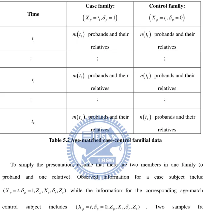
5.2 Likelihood Analysis Based on Familial Data
Table 5.2 summarizes observed case-control familial data in which probands’ times
(onset or censored) are matched. Specifically at time t , we sample i m t case probands
iand their relatives and matched with n t control probands and their relatives. Denote
i ( p, r)X X X as observed times and ( p, r) as the corresponding indicators for a proband and his/her relative respectively.
Time Case family:
Xp ti,p 1
Control family:
Xp ti,p 0
1t m t probands and their
1relatives
1n t probands and their
relatives
i
t m t probands and their
irelatives
in t probands and their
relatives
k
t m t
k probands and theirrelatives
kn t probands and their relatives
Table 5.2 Age-matched case-control familial data
To simply the presentation, assume that there are two members in one family (one
proband and one relative). Observed information for a case subject includes
(Xp t,p 1,Zp,Xr,r,Zr) while the information for the corresponding age-matched control subject includes (Xp t,p 0,Zp,Xr,r,Zr) . Two samples from
Pr( Xr,r ,Z Zp, r | Xp t,p 1 ) and Pr(
Xr,r
,Z Zp, r |
Xp t,p 0 )
are drawnindependently.
Li et al. (1998) extended the discussions in Whittemore (1995) from binary data to
age-onset data. The model assumption consists of two stages. In the first stage, the model on
the proband namely Pr(Zp|