Transient behaviors of surface plasmon coupling with a light emitter
Wen-Hung Chuang, Jyh-Yang Wang, C. C. Yang,a兲and Yean-Woei Kiangb兲
Institute of Photonics and Optoelectronics and Department of Electrical Engineering, National Taiwan University, 1, Roosevelt Road, Section 4, Taipei 10617, Taiwan
共Received 23 July 2008; accepted 20 September 2008; published online 13 October 2008兲 The transient behaviors of dipole couplings with surface plasmons 共SPs兲 on a metal/dielectric grating interface, including surface plasmon polariton共SPP兲 and localized surface plasmon 共LSP兲, are numerically demonstrated. Such a dipole-SP coupling process can lead to either enhanced dipole emission or effective pumping of a cavity-confining SP mode. Based on the time-resolved responses of a source pulse, it is found that the dipole-SP coupling features can be excited in several femtoseconds with the decay times ranging from 5 to 20 fs. From the significantly different decay times between the LSP and grating-assisted SPP features, one can classify those SP-coupling features into different application categories of efficient emission and SP energy storage. © 2008 American Institute of Physics. 关DOI:10.1063/1.2998617兴
The coupling of a radiation dipole with a surface plas-mon 共SP兲 generated on a nearby metal surface can lead to effective energy transfer from the dipole into the SP. This may have the application of emission enhancement or effec-tive SP energy pumping.1–9 The emission enhancement mechanism of SP coupling is useful for improving the effi-ciency of a light-emitting device. On the other hand, effec-tive SP energy pumping is a crucial factor for implementing a system of SP amplification by stimulated emission of ra-diation 共SPASER兲 besides the requirement of an effective SP-confining cavity.10,11 The SP coupling with a radiation dipole is an effective approach for pumping SP energy. In either application, a metal grating of an appropriate period with properly designed groove geometry has been considered for use in supporting SPs.6,7,12–15 The grating period is de-signed to match the momentum between surface plasmon polariton 共SPP兲 and photon for effective coupling and/or emission. The design of the metal groove geometry aims at the generation of localized surface plasmons 共LSPs兲 for ef-fective coupling and/or emission. Also, a metal grating of appropriate geometry can be a good choice for forming an effective SP-confining cavity in the effort of implementing a SPASER system.16 Although the SPP coupling in a metal grating structure has been widely discussed, the effect of LSP coupling in a similar structure was rarely studied. Also, although SP couplings with a quantum well or a dipole have been widely studied, they are limited to the frequency re-sponse. Transient behaviors of such a coupling process have not been reported yet. Such a study can help in elucidating the effectiveness of SP energy storage in an SP-dipole cou-pling system. It is useful for designing a metal nanostructure for either emission enhancement or SPASER implementa-tion.
In this letter, we report the numerical simulation results on the transient behaviors of such a SP-dipole coupling pro-cess. The time-response functions at a few near-field loca-tions of a pulsed radiation dipole located near a metal grating interface are evaluated. To simulate the transient field re-sponses, we first calculate the electromagnetic field
distribu-tion in the frequency domain based on the boundary integral-equation method共BIEM兲17and then take the inverse Fourier transform to obtain the time-resolved response.
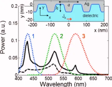
The metal grating structure under study is shown in the insert of Fig.1. Here, a periodical corrugation structure with a period a = 100 nm and the single-groove shape governed by y = −h exp共−兩x/d兩m兲 with h=10 nm, m=6.73, and d = 23.75 nm are used. The grating interface separates a half space of Ag and a half space of dielectric. For numerical computation, the permittivity of Ag is assumed to follow the Drude model18with the angular plasma frequency set at p = 1.19⫻1016 共rad s−1兲 and damping constant set at␥= 1.33
⫻1014 共rad s−1兲, leading to the SPP resonance energy at
⬃430 nm on a flat Ag/dielectric interface with the refractive index of the dielectric fixed at 2.5. A radiation dipole ori-ented along the x axis and labeled as Jxis placed at a position of 10 nm below a grating valley at x = 0. The dipole and the grating structure are assumed to be infinitely extended along the +z and −z directions for defining a two-dimensional
a兲Electronic mail: [email protected]. b兲Electronic mail: [email protected].
FIG. 1.共Color online兲 Dipole radiation power spectrum 共continuous curve兲, the emission spectrum of the SP-dipole coupling system共dashed curve兲, and the three source spectra共dotted Gaussian-like curves labeled as 1–3兲. The insert shows the two-dimensional Ag/dielectric grating structure in the x-y plane. The dipole Jxis located 10 nm right below the center of a grating
groove.
APPLIED PHYSICS LETTERS 93, 153104共2008兲
0003-6951/2008/93共15兲/153104/3/$23.00 93, 153104-1 © 2008 American Institute of Physics
problem. The two-dimensional problem geometry is reason-able for our study as we are mainly concerned with the grating-assisted SPP along the x axis and the z-invariable LSP features.
The continuous and dashed curves in Fig. 1 show the radiation power spectra of the dipole and the coupling-system emission, respectively. The dipole radiation power is obtained by integrating the outgoing Poynting vectors from a square boundary of 2.5 nm in dimension with the dipole at the center. It represents the dipole output under the SP-coupling condition. The system emission power is obtained by integrating the Poynting vectors in the −y direction along a horizontal line 1 m共far field兲 below the dipole. The sys-tem emission power is lower than the dipole radiation power due to the energy loss of metal dissipation and the SPP propagation along the⫾x directions. The three major dipole radiation features in Fig. 1are labeled as 1–3. Three source spectra of the same frequency distribution are defined for the three SP features, as depicted by the three dotted Gaussian-like curves in Fig. 1. The single-frequency field-magnitude 共absolute value of Hz兲 distributions of features 1–3 are shown in Figs. 2共a兲–2共c兲, respectively. Except feature 3, the coupling field distributions are localized indicating their LSP natures. The evaluated outward power flows along the Ag/ dielectric interface of features 1 and 2 are negligibly small, confirming that they are LSP features. Feature 3 shows a broad field distribution in the x-y plane, indicating its grating-assisted SPP characteristics. It is noted that the weak
emission of this SP feature共see Fig.1兲 does not guarantee its effective SP energy storage. Other loss mechanisms, includ-ing SPP outward propagation along the interface and metal dissipation, may rapidly decrease SP energy. The locations labeled as A1–3, B1–3, C3, and D3 in Figs. 2共a兲–2共c兲are
as-signed as the observation points of the time-resolved study. Points A1–3 are located at the Ag/dielectric interface right above the dipole. Points A3-D3are separated successively by one grating period.
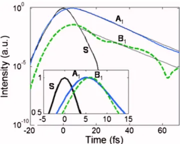
Figure 3 shows the time-resolved intensity profiles of feature 1 共LSP兲 at the two observation points. Here, the source profile is also shown and labeled as S for reference. The intensity profiles at those observation points are normal-ized to the peak level at point A1, which is normalized to the
source peak level. The intensity profiles in a linear scale and normalized by the individual peak levels are shown in the insert. The response delay times from the source peak and the profile decay times are shown in TableI. The delay times at A1 共5.39 fs兲 and B1 共5.74 fs兲 represent the characteristic
time constant for building the coupling system of feature 1. The fitted decay times of those profiles show the similar decay slopes, indicating that after the coupling system is built, the system releases energy with an effective decay time of ⬃7–8 fs.
Figure 4 shows the time-resolved intensity profiles of feature 2 共LSP兲 at the two observation points. Although the peak at A2can appear in a short time共2.92 fs兲, it takes ⬃7 fs
for building the complete field distribution of the coupling system. The relatively shorter decay times in comparison to FIG. 2. 共Color online兲 Single-frequency field magnitude distributions of
features 1–3 in parts关共a兲–共c兲兴, respectively. The labeled positions are con-sidered for transient study.
FIG. 3. 共Color online兲 Time-resolved field intensity profiles at various ob-servation points for feature 1. The inset at the bottom shows the linear-scale profiles for demonstrating the temporal peak positions.
TABLE I. Time-resolved signal parameters of the three SP-dipole coupling systems.
Observation point A1,2,3 B1,2,3 C3 D3
Feature 1 Delay time共fs兲 5.39 5.74 ¯ ¯
共430 nm兲 Decay time共fs兲 6.92 7.55 ¯ ¯
Feature 2 Delay time共fs兲 2.92 7.15 ¯ ¯
共520 nm兲 Decay time共fs兲 5.56 5.09 ¯ ¯
Feature 3 Delay time共fs兲 1.12 9.33 14.32 19.26
共590 nm兲 First decay time共fs兲 4.11 13.11 13.09 14.32 Second decay time共fs兲 18.95 20.69 20.32 19.62
153104-2 Chuang et al. Appl. Phys. Lett. 93, 153104共2008兲
feature 1 of ⬃5 fs at both observation points of this LSP feature are attributed to the more effective emission of this coupling system because the dissipation rates of the two LSP features, which are defined by the fixed metal damping factor
␥, are supposed to be similar.
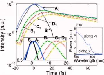
Figure 5 shows the time-resolved intensity profiles of feature 3 共grating-assisted SPP兲 at the four observation points. Here, effective coupling leads to a short buildup time at A3 共1.12 fs兲. At B3-D3, energy is received mainly through
SP outward propagation from A3. Therefore, the peaks at C3
and D3appear at about 5 and 10 fs later than that at B3. We have used the plane-wave-assisted BIEM17to plot the disper-sion curve of the concerned SPP. From the disperdisper-sion curve of feature 3, we can evaluate the group velocity of this SPP at 590 nm to give 1.99⫻107 m/s. The propagation of this
SPP over a grating period共100 nm兲 with this group velocity accounts for the observed ⬃5 fs successive delays between B3, C3, and D3. The longer delay at B3is due to the required
period for building the local coupling. In Fig. 5, two decay
components can be seen in all the response profiles. The first-stage decay is attributed to the outward SPP propagation from A3. This stage ends when the intensity at B3is about the same as that at A3. At this moment, the counterpropagation
through grating diffraction results in negligible energy trans-port from a grating element into the neighboring ones. In the inset at the lower-right corner of Fig. 5, we compare the along-interface outward propagating power 共along x兲 at x =⫾500 nm and the emission power 共along −y兲 at 590 nm to show the much weaker along-interface propagation. There-fore, the SP energy in this grating-assisted SPP feature is well confined. The long decay time of⬃20 fs in the second decay stage implies that such a SP feature has the potential of implementing a SPASER system. On the other hand, the two LSP-coupling features are useful for enhancing the efficiency of a light-emitting device.
In summary, we have demonstrated the transient behav-iors of the dipole couplings with three SP features. The sig-nificantly longer decay time 共in the second decay stage兲 of the grating-assisted SPP feature implied its potential applica-tion to SPASER implementaapplica-tion, while the efficient emis-sions and hence the shorter decay times of the LSP-coupling features implied their effective applications to emission en-hancement.
This research was supported by the National Science Council, The Republic of China, under Grant Nos. NSC 96-2120-M-002-008 and NSC 96-2221-E-002-188 and by the U.S. Air Force Scientific Research Office under Contract No. AOARD-07-4010.
1A. Neogi, C. W. Lee, H. O. Everitt, T. Kuroda, A. Tacheuchi, and E.
Yablonovitch,Phys. Rev. B 66, 153305共2002兲.
2K. T. Shimizu, W. K. Woo, B. R. Fisher, H. J. Eisler, and M. G. Bawendi,
Phys. Rev. Lett. 89, 117401共2002兲.
3Y. Ito, K. Matsuda, and Y. Kanemitsu,Phys. Rev. B 75, 033309共2007兲. 4M. A. Noginov, G. Zhu, M. Bahoura, C. E. Small, C. Davison, J.
Ade-goke, V. P. Drachev, P. Nyga, and V. M. Shalaev,Phys. Rev. B 74, 184203 共2006兲.
5K. Okamoto, I. Niki, A. Shvartser, Y. Narukawa, T. Mukai, and A.
Scherer,Nature Mater. 3, 601共2004兲.
6G. Sun, J. B. Khurgin, and R. A. Soref, Appl. Phys. Lett. 90, 111107
共2007兲.
7J. B. Khurgin, G. Sun, and R. A. Soref, J. Opt. Soc. Am. B 24, 1968
共2007兲.
8D. M. Yeh, C. F. Huang, C. Y. Chen, Y. C. Lu, and C. C. Yang, Appl.
Phys. Lett. 91, 171103共2007兲.
9D. M. Yeh, C. F. Huang, C. Y. Chen, Y. C. Lu, and C. C. Yang,
Nanotechnology 19, 345201共2008兲.
10D. J. Bergman and M. I. Stockman,Phys. Rev. Lett. 90, 027402共2003兲. 11J. Seidel, S. Grafström, and L. Eng,Phys. Rev. Lett. 94, 177401共2005兲. 12J. Y. Wang, Y. W. Kiang, and C. C. Yang,Appl. Phys. Lett. 91, 233104
共2007兲.
13K. C. Shen, C. Y. Chen, C. F. Huang, J. Y. Wang, Y. C. Lu, Y. W. Kiang,
C. C. Yang, and Y. J. Yang,Appl. Phys. Lett. 92, 013108共2008兲.
14W. H. Chuang, J. Y. Wang, C. C. Yang, and Y. W. Kiang,Appl. Phys. Lett.
92, 133115共2008兲.
15W. H. Chuang, J. Y. Wang, C. C. Yang, and Y. W. Kiang,IEEE Photonics
Technol. Lett. 20, 1339共2008兲.
16Y. Gong and J. Vučković,Appl. Phys. Lett. 90, 033113共2007兲. 17J. Y. Wang, C. C. Yang, and Y. W. Kiang,Opt. Express 15, 9048共2007兲. 18F. Wooten, Optical Properties of Solids共Academic, New York, 1972兲.
FIG. 4. 共Color online兲 Similar to Fig.3except for feature 2.
FIG. 5. 共Color online兲 Similar to Fig.3except for feature 3. In the inset at the lower-right corner, we compare the along-interface outward propagating power共along x兲 at x= ⫾500 nm and the bottom emission power 共along −y兲 at 590 nm in wavelength.
153104-3 Chuang et al. Appl. Phys. Lett. 93, 153104共2008兲