高解析度距離都普勒雷達成像流程研究

國 立 交 通 大 學

機械工程學系

碩士論文

高解析度距離都普勒雷達成像流程研究

Research of High Resolution Range-Doppler Radar Imaging

Procedure

研 究 生： 侯俊仰

指導教授： 成維華 教授

高解析度距離都普勒雷達成像流程研究

Research of High Resolution Range-Doppler Radar Imaging Procedure

研 究 生：侯俊仰 Student：Ching-Yang Hou 指導教授：成維華 Advisor：Dr. Wei-Hua Chieng

國 立 交 通 大 學 機 械 工 程 學 系

碩 士 論 文

A Thesis

Submitted to Institute of Mechanical Engineering College of Engineering

National Chiao Tung University in partial Fulfillment of the Requirements

for the Degree of Master

in

Mechanical Engineering

July 2007

Hsinchu, Taiwan, Republic of China

高解析度距離都普勒雷達成像流程研究

摘 要

Research of High Resolution Range-Doppler Radar Imaging Procedure

Student：Ching-Yang Hou Advisor：Dr. Wei-Hua Chieng

Institute of Mechanical Engineering National Chiao Tung University

Abstract

Range-Doppler radar can produce two-dimension imagery of the ground surface versus range and azimuth axis. The quality of ground maps generated by

Range-Doppler radar is determined by the size of the resolution cell. A resolution cell is specified by both range and azimuth resolution of the system.

Fine range resolution can be accomplished by using pulse compression techniques. The azimuth resolution depends on antenna size and radar

wavelength of operation band. In radar range processing, it usually emphasizes the signal to noise ratio to be maximum and utilizes the linear frequency

modulation to accomplish the pulse compression. However, it is utilizing the motion of antenna versus the Doppler effect of targets to produce the purpose of

linear frequency modulation in azimuth processing.

The range and azimuth processing have the same mathematical modal, but

have the different physical characteristics and meaning. Basing on the principle of range compression and azimuth compression, the main purpose is to construct

a procedure of Strip-map microwave radar by using simulation of point target in this paper.

誌謝 首先要感謝我的指導老師 成維華 教授，讓我加入了實驗室，在這兩年 的碩士生涯中，無論是在學業、生活、或是待人處事等方面，都不厭其煩 的給予我指導與教誨，也從中獲得了啟發與智慧，在我踏入社會之前，給 了我嚴格的磨練，我相信在近入職場後，有自信去面對各種問題，且都能 找出解決的方法。 這個研究的完成，特別要感謝楊嘉豐學長對我的指導，對於反應不快的 我，依然是很有耐心地把我從無教到有，在這兩年裡，也因學長亦師亦友 的指導，我才能順利的畢業。 實驗室的氣氛一直都是很愉快地，很高興能認識童永成學長、張仰宏學 長、以及吳秉霖學長，因為學長們的熱情，讓我感到實驗室的溫馨，偉鈞、 明亮、明欣、建成，跟你們一起渡過了兩年吃喝拉撒吃喝拉睡都在一起的 生活，這段同甘共苦的日子，我相信一定很難忘懷，情和義，值千金。 謝謝我的父母能夠支持我選擇的路，在這段日子裡，無論是生活或是 心理方面，都能完完全全的支持我，而我也沒有讓你們失望，得到了碩士 學位，謝謝你們，我只想跟你們說：「爸、媽，我在這裡，我畢業了」。也 謝謝我的女朋友，我最艱困的日子裡，依然無怨無悔的陪在我身邊。 最後感謝所有曾經幫助過我的人以及我在交大認識的朋友，謝謝你們。

Contents

List of Tables……….. vii

Chapter 1 Introduction………. 1

1.1 History……… 1

1.2 Motive and Object……….. 2

1.3 Research Orientation……….. 3

Chapter 2 Range processing………. 4

2.1 Basic of Range Processing………. 4

2.1.1 Range Resolution………. 4

2.1.2 Linear Frequency Modulation Waveforms………... 5

2.1.3 Correlation and Convolution……… 6

2.2 The Matched Filter………. 8

2.3 LFM Pulse Compression……… 9

2.3.1 Correlation Processor………... 12

2.3.2 Time Interval of Sampling……… 15

2.3.3 Range Sampling Criteria……….. 18

2.4 Simulation for Range Processing………... 19

Chapter 3 Azimuth processing………. 20

3.1 Azimuth Resolution……… 20

3.2 Properties of Echo Signal……….……….………. 22

3.3 Azimuth Compression……….………... 28

3.4 Azimuth Sampling Criteria………. 30

3.5 Simulation for Azimuth Processing……… 31

Chapter 4 Stripmap Range-Doppler Radar Imaging Procedure………….. 32

4.1 Raw Data……… 32

4.2 Imaging Procedure……….. 33

4.3 Simulation for Point Target………. 34

4.4 Compensation with Variable PRF……….. 34

Chapter 5 Conclusion……… 36

List of Figures

Figure 2-1 (a) Two unresolved targets. (b)Two resolved targets…………... 38

Figure 2-2 Typical LFM waveforms. (a) Up-chirp; (b) Down-chirp………. 38

Figure 2-3 Correlation………... 39

Figure 2-4 Relationship between Multiplication and Convolution………... 39

Figure 2-5 Convolution……….. 40

Figure 2-6 Matched filter definitions………. 40

Figure 2-7 Ideal LFM pulse compression……….. 41

Figure 2-8 LFM pulse after matched filter……… 41

Figure 2-9 Computing the matched filter output using an FFT………. 42

Figure 2-10 System geometry for range imaging……… 42

Figure 2-11 Scenery of example in range processing……….. 43

Figure 2-12 First method of range processing………. 43

Figure 2-13 Second method of range processing……… 43

Figure 2-14 Real part and spectrum of transmit signal……… 44

Figure 2-15 Real part and spectrum of reference signal……….. 44

Figure 2-16 Receive signal and Compressed echo signal………... 45

Figure 3-1 Application of airborne Range-Doppler radar………. 45

Figure 3-2 Airborne Range-Doppler radar Geometry………... 46

Figure 3-3 Properties of frequency and phase between transmit signal and echo signal………... 46

Figure 3-4 Relationship between target location and Doppler frequency 47 Figure 3-5 Scenery of example in azimuth processing……….. 47

Figure 3-6 Real part and spectrum of reference signal in azimuth direction. 48 Figure 3-7 Receive signal and compressed signal in azimuth direction…… 48

Figure 4-1 Transmitted and received signal in Range-Doppler radar……… 49

Figure 4-2 The diagram of raw data……….. 49

Figure 4-3 Fast correlation with one-dimensional reference signal……….. 50

Figure 4-4 Range-Doppler radar imaging procedure………. 50

Figure 4-5 Raw data with one point target……… 51

Figure 4-6 Image after range compression and correction……… 51

Figure 4-7 Range-Doppler radar image with one target……… 52

Figure 4-8 -4dB Contour for one point target……… 52

Figure 4-9 Range-Doppler radar image in azimuth with one target……….. 53

Figure 4-10 Range-Doppler radar image in ground range direction………... 53

Figure 4-13 -4dB Contour with multiple targets with multiple targets……... 55 Figure 4-14 The motion error between actual and nominal trajectory……… 55 Figure 4-15 The diagram of fixed PRF and variable PRF………... 56 Figure 4-16 The Scenery illuminated by Range-Doppler radar……….. 56 Figure 4-17 Actual and nominal flight path……… 57 Figure 4-18 The image after range compression with nominal path………... 58 Figure 4-19 Range-Doppler radar image with nominal path………... 58 Figure 4-20 Range-Doppler radar image with actual path……….. 59 Figure 4-21 Range-Doppler radar image after LOS compensation…………. 59

List of Tables

Table 2-1 Parameters for range processing……….. 60

Table 3-1 Parameters for azimuth processing……….. 60

Table 4-1 Parameters for one point target simulation……….. 61

Table 4-2 Parameters for multiple point target simulation………... 61

Chapter 1 Introduction

The word radar is an abbreviation for RAdio Detection And Ranging. In

general, radar system use modulated waveforms and directive antennas to transmit electromagnetic energy into a specific volume in space to search for

targets. Objects within a search volume will reflect portions of this energy back to the radar. These echoes are then processed by the radar receiver to extract

target information such as range, velocity, angular position, and target identifying characteristics.

1.1 Historical Reviews

The Synthetic Aperture Radar (SAR) concept is usually attributed to Carl

Wiley of Goodyear Aircraft Corporation in 1951 (and subsequently patented in 1965 [Wiley, 1965]). However its first experimental validation was carried out

in 1953 by a group of scientists at the University of Illinois (Sherwin et al., 1962); later on, the U.S. Army commissioned Project Wolverine on this subject

to the University of Michigan. The University of Illinois, General Electric Company, Philco, Varian, and Goodyear Aircraft Corporation joined the project.

This was the beginning of a series of activities that contributed to the development of SAR techniques.

The first operational SAR system is believed to be builted in 1957 by Willow Run Laboratories of the University of Michigan (currently

Environmental Research Institute of Michigan [ERIM]) for the U.S. Department of Defense [DoD]. A large part of early activities in this field is still classified,

and related information is not available. However, starting from the end of the 1960s, NASA began to sponsor the development of SAR systems for civilian

applications. One of the first consisted of the modification of a system originally developed by ERIM and was declassified at the end of the 1960s. This system

was later upgraded by NASA in 1973 by the addition of an L-band.

1.2 Motive and Object

SAR imaging technique is related with electronic engineering, computer science and digital signal processing. The appearing and development of SAR

enlarge the traditional radars’ application. With the development of SAR imaging technique and the improvement of SAR imaging quality, high range

and azimuth resolution has come true. As a result, SAR has been an important tool for scientific research and remote sensing. It will take on a supreme future

in both military and economy.

Radar users and designers alike seek to accomplish high resolution by

minimizing range resolution and azimuth resolution. In order to achieve high range resolution one must use very short pulses and consequently reduce the

average transmitted power and impose severe operating bandwidth requirements. High resolution SAR requires more complex hardware implementation and costs

helpful to make the system more complete. For this reason, it is necessary to analyze and test through the simulation of airborne Strip-map SAR system.

1.3 Research Orientation

This paper introduces firstly the basic principle behind one-dimensional

range imaging via utilization of a radar bandwidth in chapter 2. Result shows that the algorithm to matched filtering imaging is very good by analyzed,

because the signal matched to the echo of targets includes not only phase but amplitude information. Basing on this, the algorithm about azimuth imaging via

utilization of a synthetic aperture is analogized in chapter 3. These basic principles, and their associated data acquisition and digital signal processing

issues, will assist us in developing more concrete high resolution SAR.

Chapter 4 discusses system modeling and imaging for broadside strip-map

SAR within the framework of the spectral properties of the SAR radiation pattern that is developed in chapter 3. At the same time, the conclusion is

validated by use of computer simulation. Then, the relationship between the trajectory and resolution can be analyzed as a result of the strip-map SAR

Chapter 2 Procedure of Range Processing

For older radar systems where no pulse compression was possible, the range resolution was improved by reducing the pulse length. The disadvantage is

that the transmitted power is also decreased which is directly linked to the signal to noise ratio (SNR). By instead transmitting frequency modulated pulses and

using pulse compression techniques, the pulse length can be increased and still achieve fine range resolution.

2.1 Basics of Range Processing

2.1.1 Range Resolution

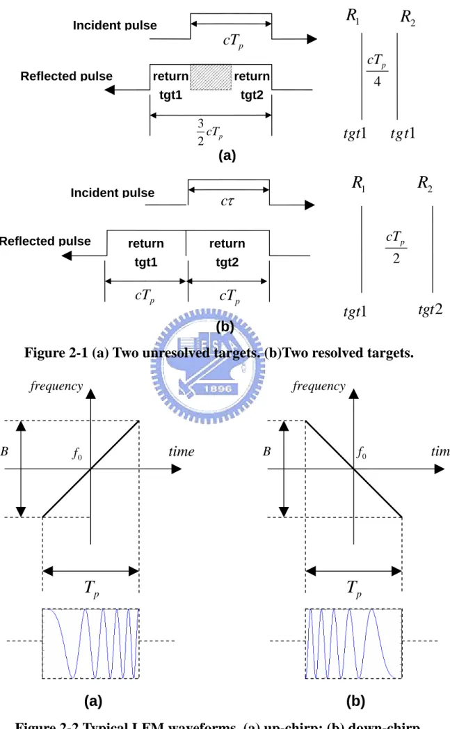
Range resolution, denotes as ΔR, is a radar metric that describes its ability to detect targets in lose proximity to each other as distinct objects. Targets

separated by at least ΔR will be completely resolved in range.

Assume that the two targets are separated by cT_p / 4, where Tp is the

pulsewidth. In this case, when the pulse trailing edge strikes target 2 the leading

edge would have traveled backwards a distance cTp, and the returned pulse

would be composed of returns from both targets, as shown in Fig. 2-1a.

However if the two targets are at least cT_p / 2 apart, then as the pulse trailing edge strikes the first target the leading edge will start to return from target 2, and two distinct returned pulses will be produced, as illustrated by Fig. 2-1b. Thus,

R

Δ should be greater or equal to cTp / 2. And since the radar bandwidth B

is equal to 1/Tp , then 2 2 p cT _c R B Δ = = _(2-1)

2.1.2 Linear Frequency Modulation Waveforms

Frequency or phase modulated waveforms can be used to achieve much

wider operating bandwidths. Linear Frequency Modulation (LFM) [1] is

commonly used. In this case, the frequency is swept linearly across the pulsewidth, either upward (up-chirp) or downward (down-chirp). The matched

filter bandwidth is proportional to the sweep bandwidth, and is independent of the pulsewidth. Fig. 2-2 shows a typical example of an LFM waveform. The

pulsewidth is Tp, and the bandwidth is B.

The LFM up-chirp instantaneous phase can be expressed by

2 ( ) 2 ( ) 2 c k t f t t

ψ

π

where fc is the radar center frequency, and K =(2

π

τ

coefficient. Thus, the instantaneous frequency is

1 d

_ψ

Atypical LFM waveform can be expressed by 2 2 ( ) 2 1( ) Rect( ) c k j f t p t s t e T π + = _(2-4) where Rect( t ) p

T denotes a rectangular pulse of width Tp.

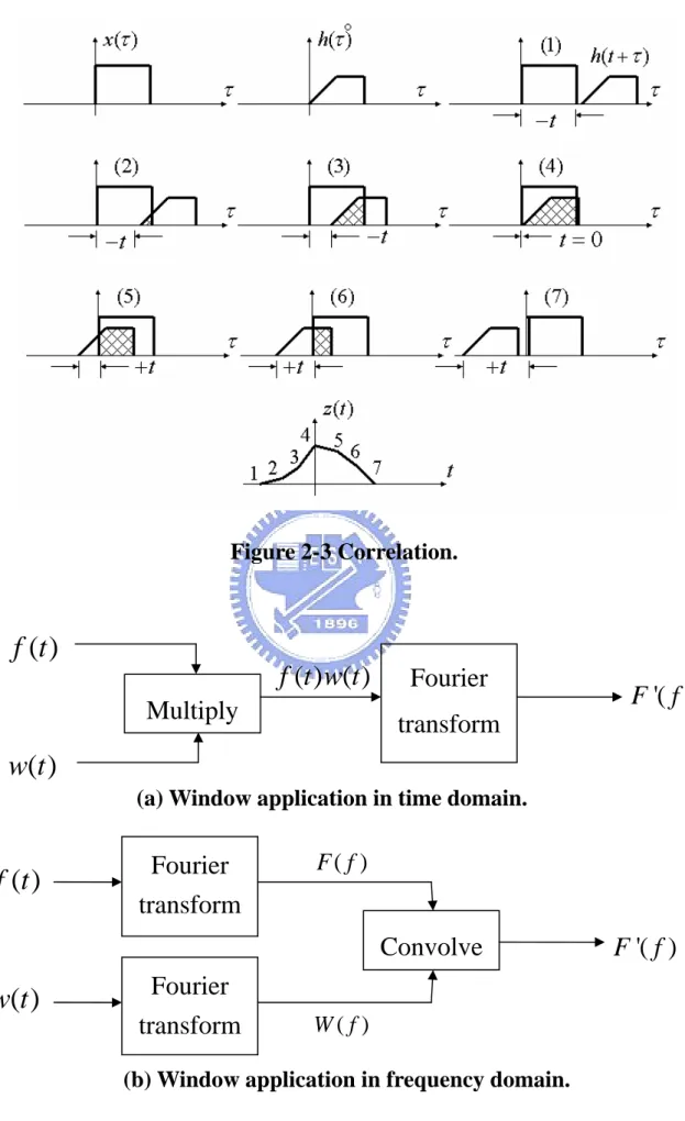
2.1.3 Correlation and Convolution

Correlation[2] is the process of matching two waveforms, usually in the

time domain, to determine their degree of fit and to determine the time at which the maximum correlation coefficient, or best fit, occurs. Correlation can occur in

either the continuous or discrete realms.

This correlation from involves signals which are continuous and periodic.

A mathematical description of continuous correlation is

( ) ( ) ( ) ( ) ( )

z t x t h t ∞ x

τ

τ τ

−∞

= ⊗ =

∫

In the process, one signal [x( )

τ

τ

The parameter t represents the amount of displacement of h from its normal

time position where t =0. Note that on the right of the equation, t is a parameter; on the left, it is a variable. Thus the process is truly a transform in that it changes the independent variable. The correlation process is shown in Fig.

2-3.

Two types of correlation exist. If the two waves being matched are

different, x t( )≠h t( ), a cross-correlation is performed. If they are the same,

( ) ( )

x t =h t , it is an autocorrelation. Autocorrelation are used to evaluation the suitability of waveforms to certain radar tasks and cross-correlation are used primarily in pulse compression.

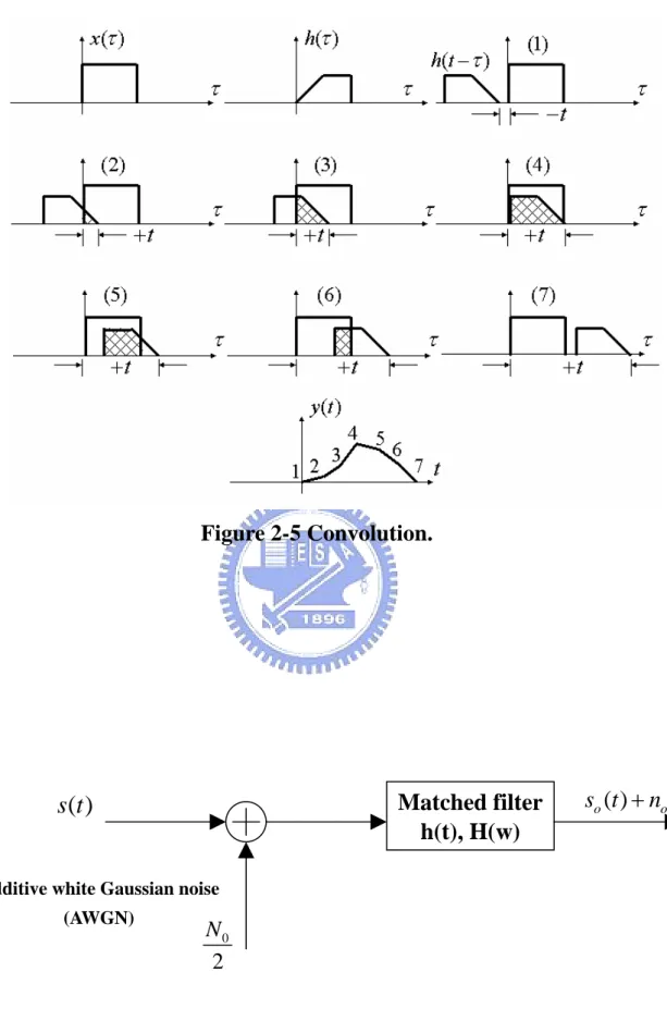
Convolution is a process by which multiplications are transferred from one domain to the other. The relationship between multiplication and convolution is

given below and in Fig. 2-4.

[ ( ) ( )] [ ( )] [ ( )] ( ) ( )

FT f t w ti = FT f t ∗FT w t = F f ∗W f (2-6)

The process of convolution is almost identical to that of correlation. The

only difference is that one of the signals (it makes no difference which one) is reversed, or folded, in time before the displace-multiply-integrate operations.

Convolution of continuous functions is given below

( ) ( ) * ( ) ( ) ( )

z t x t h t ∞ x

τ

τ τ

−∞

= =

∫

Graphically, convolution is shown in Fig. 2-5. Note its similarity to

2.2 The Matched Filter

In radar applications we generally utilize the reflected known signal to detect the existence of a reflecting target. The probability of detection is related

to the signal to noise ratio (SNR) rather than to the exact waveform of the signal received. Hence we are more interested in maximizing the SNR than in

preserving the shape of the signal. A specific matched filter is a linear filter whose impulse response is determined by a specific signal in a way what will

result in the maximum attainable SNR at the output of the filter when that particular signal and white noise are passed through the filter.

Matched filter[3] can be derived for baseband as well as for bandpass real

signals. For the latter case it will usually suffice to implement a filter matched to the complex of signal. Hence, we need to be able to design matched filters for

complex signals as well.

The impulse response of the matched filter is

* 0

( ) ( )

h t = Ks t −t (2-8)

This says that the impulse response is a delayed mirror image of the conjugate of the signal.

It can easily be derived using convolution between the signal and the matched filter impulse response,

* 0 ( ) ( ) * ( ) ( ) ( ) ( ) [ ( )] o s t s t h t ∞ s

τ

τ τ

τ

τ τ

∫

∫

If we assume that t0 =0 and K =1, then * ( ) ( ) ( ) o s t ∞ s

τ

τ

τ

∫

the right-hand side of Eq. (2-10) is recognized as the autocorrelation function of

( )

s t .

We can now summarize the main results concerning the matched filter: The

impulse response is linearly related to the time-inverted complex-conjugate signal; when the input to the matched filter is the correct signal plus white noise,

the peak output response is linearly relate to the signal’s energy. At that instance,

the SNR is the highest attainable, which is 2 /E N0; elsewhere, the response is

described by the autocorrelation function of the signal.

2.3 LFM Pulse Compression

Linear frequency modulation pulse compression is accomplished by adding

frequency modulation to a long pulse at transmission, and by using a matched filter receiver in order to compress the received signal.

The matched filter impulse response of s t( ) is

*

( ) ( )

h t = s −t (2-11)

2 2 ( ) Rect( ) j f tc j kt p t h t e e T π − π = _(2-12)

Then, the output signal s t_o( ) of s t( ) passing through the system h t( ) is

( ) ( ) * ( ) o s t =s t h t ( ) ( ) s u h t u du ∞ −∞ =

∫

∫

∫

∫

π

π

π

∫

2 2 ₂ 2 c j ktu j f t j kt T t T e e e j kt π π π

π

π

π

Combining Eq. (2-13) with Eq. (2-14) yields

2 | | sin (1 ) t ( ) Rect( ) 2T c j f t o t kT t T s t T e kTt π

π

π

Eq. (2-15) is the output of LFM signal passing through the matched filter. It is a

signal of fixed carrier frequency fc.

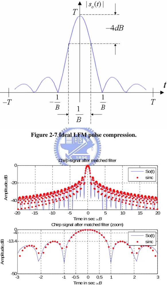
When t ≤Tp, the envelope is similar to a sinc function

t t ( ) ( )Rect( ) ( )Rect( ) 2T 2T o s t =TSa

π

π

= ± _{is the first zero point when}

_π

_π

When 2 Bt

π

π

= ± _{.It is usually to define the presently pulsewidth as}

the compressed pulsewidth

1 1

2 2B x B

As a result, the matched filter output is compressed by a factor

ξ

where

τ

The time axis is normalized in Fig. 2-8, (t/(1/ )B = ×t B). The result simulated in Fig. 2-8 is as good as the theory. The relative amplitude is -13.4 dB

when the first zero point appears at ±1 ( 1

B

± _{). As illustrated in Fig. 2-9, it is}

equal to the analysis in theory and the relative amplitude is -4dB when the

compressed pulsewidth is similar to 1

B (

1 2B ± _).

2.3.1 Correlation Processor

Radar operations area usually carried out over a specified range window,

referred to as the receive window and defined by the difference between the radar maximum and minimum range. Returns from all targets within the receive

window area collected and passed through matched filter circuitry to perform pulse compression. One implementation of such analog processors is the Surface

Acoustic Wave (SAW) devices. Because of the recent advances in digital

computer development, the correlation processor[4] is often performed digitally

using FFT. This digital implementation is called Fast Convolution Processing

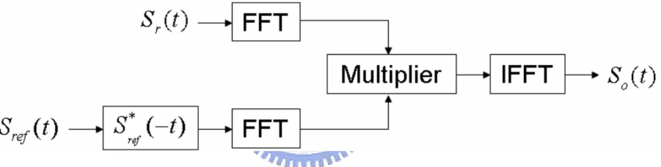
(FCP) and can be implemented at base-band. The fast convolution process is illustrated in Fig. 2-9.

Since the matched filter is a linear time invariant system, its output can be described mathematically by the convolution between its input and its impulse

response,

( ) ( ) ( )

y t =s t ∗h t (2-18)

where s t( ) is the input signal, h t( ) is the matched filter impulse

response(reference signal), and the ∗ operator symbolically represents convolution. From the Fourier transform properties,

{ ( ) ( )} ( ) ( )

FFT s t ∗h t =S f iH f (2-19)

and when both signals are sampled properly, the compressed signal y t( ) can

be computed from

1

( ) { ( ) ( )}

y t = FFT− S f iH f (2-20)

where FFT−1 is the inverse FFT. When using pulse compression, it is

desirable to use modulation schemes that can accomplish a maximum pulse compression ratio, and can significantly reduce the sidelobe levels of the

compressed waveform. For the LFM case the first sidelobe is approximately 13.4dB below the main peak, and for most radar applications this may not be

sufficient. In practice, high sidelobe levels are not preferable because noise and/or jammers located at the sidelobes my interfere with target returns in the

Weighting function (windows) can be used on the compressed pulse spectrum in order to reduce the sidelobe levels. The cost associated with such an

approach is a loss on the main lobe resolution, and a reduction in the peak value. Weighting the time domain transmitted or received signal instead of t he

compressed pulse spectrum will theoretically achieve the same goal. However, this approach is rarely used, since amplitude modulating the transmitted

waveform introduces extra burdens on the transmitter.

Consider a radar system that utilizes a correlation processor receiver. The

receive window in meters is defined by

rec max min

R = R −R (2-21)

where Rmax and Rmin, respectively, define the maximum and minimum range

over which the radar performs detection. Typically Rrec is limited to extent of

the target complex. The normalized complex transmitted signal has the form

2 ( ) exp 2 ( ) 2 c k s t = ⎡_⎢j

π

T is the pulsewidth, k = B T/ _p, and B is the bandwidth.

The radar echo signal is similar to the transmitted one with the exception of a time delay and an amplitude change that correspond to the target RCS.

2 1 1 1 ( ) exp 2 ( ( ) ( ) ) 2 r c k s t =a ⎡_⎢j

π

τ

τ

τ

τ

where a1 is proportional to target RCS, antenna gain, and range attenuation.

The time delay

τ

1 2R c1/

τ

This is accomplished by missing s t_r( ) with a reference signal whose phase is

2

π

ψ

π

τ

τ

and the instantaneous frequency is

1 1 2 1 ( ) ( ) ( ) ( ) 2 i p R d B f t t k t t dt

ψ

τ

π

2.3.2 Time Interval of Sampling

0 0

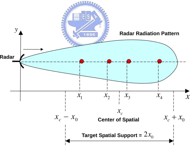
[ _c , _c ]

x∈ x −x x +x

where xc is the target area mean range and 2x0 is the size of the target area.

The echoed signal from the closest reflector at x= xc −x0 arrives at the time

0 2( _c ) start x x t c − = _(2-27)

While the echoed signal from the farthest reflector at x= xc −x0 arrives at

the receiver at the time 2(xc+x0) /c, it lasts until the time

0 2( _c ) end p x x t T c + = + _(2-28)

where Tp is the duration of the pulsed radar signal. The echoed signals that are

due to the reflectors that reside between the closest and farthest reflectors fall

between the time points Tstart and Tend.

Thus, to capture the echoed signals from all of the reflectors in the target

region x∈[xC −x x0, C +x0], we have to acquire the time samples of the echoed

signal in the following time interval[5]:

[ _start, _end]

t∈ t t

0 4 end start p x t t T c − = + _(2-29)

2.3.3 Range Sampling Criteria

The number of samples, N, must be chosen so that foldover in the spectrum

is avoided. For this purpose, the sampling frequency, fs based on the Nyquist

sampling rate, must be

2 s

f ≥ B (2-30)

and the sampling interval is

1 2 s T B ≤ _(2-31)

Using Eq. (2-26) it can be show that the frequency resolution of the FFT is

1 p

f T

Δ ≤ _(2-32)

The minimum required number of samples is

1 p s T N fT Ts = = Δ (2-33)

2 _p

N ≥ BT _(2-34)

Consequently, a total of 2BTp real samples, or BTp complex samples, is

sufficient to completely describe an LFM waveform of duration Tp and

bandwidth B . For example, an LFM signal of duration Tp =2

μ

bandwidth B=10MHz requires 40 real samples to determine the input signal. For better implementation of the FFT N is extended to the next power of

two, by zero padding. Thus, the total number of samples, for some positive integer m, is

2m FFT

N = ≥ N (2-35)

2.4 Simulation for Range Processing

As an example shown as Fig. 2-11, consider the case where the parameters

are list in table 2-1.The simulation of range processing can be achieved by using MATLAB as Fig. 2-12, and the reference signal is

(

)

π

τ

τ

τ

τ

τ

where Rmid is the center distance of receive window.

Because of the properties of Fourier transform

{ ( )} ( ) F s t = S w (2-38) { ( )} ( ) F s −t = − −S w (2-39) * * { ( )} ( ) F s t =S −w ) (2-40)

It can be known that

* *

{ ( )} ( )

F s −t = −S w (2-41)

The simulation can be achieved by another way illustrated in Fig. 2-13.

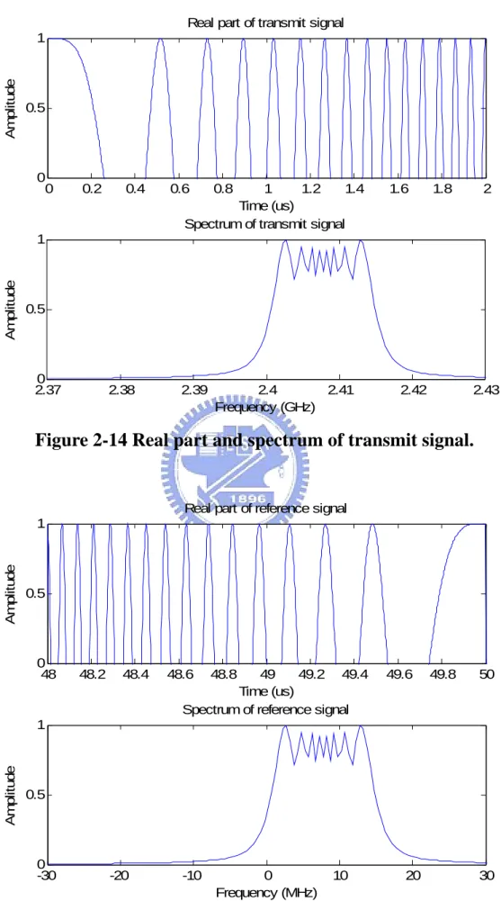
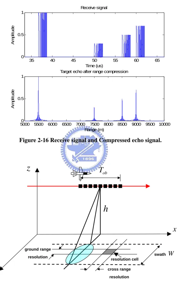
Note that the compressed pulse range resolution is ten meters. Figs. 2-14

and 2-15 show the transmit signal and reference signal respectively. Fig 2-16 shows the uncompressed echo and the compressed matched filter output.

Chapter 3 Azimuth Processing

SAR synthesize a long antenna by transmitting electromagnetic energy and coherently adding the successively reflected and received pulses to obtain high

resolution in azimuth direction. To achieve a coherent integration is called azimuth compression.

3.1 Azimuth Resolution

Azimuth (cross-range) is resolved with antenna beamwidth. The

azimuth resolution of radars are

R R A R R D

λ

θ

λ

θ

where ΔAR is the azimuth resolution using the real antenna, ΔAS is the

azimuth resolution using the synthetic antenna,

θ

θ

beamwidth of the real antenna and synthetic antenna respectively,D is the

width of the real antenna, Lsyn is the effective length of the synthetic antenna,

Azimuth resolution is enhanced by narrowing the antenna beamwidth. With real antennas, this requires enlarging the physical antenna size or decreasing

wavelength, which are often not possible because of physical constraints The same effect can be accomplished with a small real antenna moving to a number

of locations to simulate a large antenna, called a synthetic, or synthetic aperture as illustrated in Fig. 3-1.

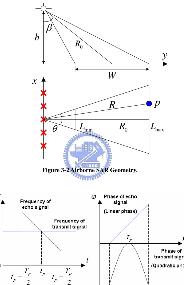
The azimuth resolution of a sidelooking SAR system is described in terms

of the geometry of Fig. 3-2. The effective length of the synthetic antenna (Lsyn)

is the distance the radar moves while a scatterer remains in the beam. It has the

same value as the azimuth resolution of the real antenna. For small real beamwidths, this value is

R syn R A L R R D

λ

θ

The azimuth resolution of the synthetic antenna at range R is, by basic resolution relationships

S S

A

θ

Δ = (3-4) Substituting Eq. (3-2) into Eq. (3-4) yields

2 S syn R A L

λ

2 S R D A R

λ

λ

Algebra reduces this equation to

2 S

D A

Δ = _(3-7)

3.2 Properties of Echo Signal

In order to make it convenient for the mathematic analysis, the geometry of

airborne SAR[6] should be discussed firstly. As illustrated in Figs. 3-1 and 3-2,

the aircraft flies along the straight line in x direction with uniform velocity v

and altitude h . The antenna of airborne SAR transmits the radio waves

broadside with regular slant angle

β

θ

The detected target is assumed as a ideal point target p and the slant

range between target pand flight path x is R0. Therefore, the coordinate

plane can be composed of flight path x and slant range R0. The aircraft is in

the origin of coordinate when t =0 and the location of aircraft is x=vt in instantaneous time t. The location of point target p in this coordinate is fixed

2 2

0 ( a p)

R= R + x −x _(3-8)

In general, R0 (xa −xp), the equation above is similar to

2 2 0 2 0 0 0 ( ) ( ) 1 2 a p a p x x x x R R R R R − − = + ≈ + _(3-9)

The high frequency pulse which is transmitted from the antenna is periodic

and coherent equally amplitude. Suppose the frequency is fc, the amplitude is

A, the pulse repeatation frequency (PRF) is fr, the repeatation period (PRT)

is r 1 r

T f

= _{, and the pulsewidth is}

_τ

transmitted from antenna is a continuous cosine wave for analysis. The actual

transmitted periodic pulse is viewed as the samples of continuous wave and its

sampling frequency is PRF fr. The amplitude of cosine wave is normalized as

1 and the beginning phase is 0. As a result, It can be expressed by using

exponential function with complex number

2 0( )

c

j f t

S t =e π _(3-10)

The signal after transmitted from antenna is a type of electromagnetic wave.

When arriving the target p, the electromagnetic wave is started to scatter, and

a part of backscatter energy is received by antenna, thus, being called echo

signal S t_r( ). Assume that the RCS of point target p is

σ

0

2 ( )

( ) j fc t

r

S t =

σ

τ

0

2R

c

τ

Substituting Eq. (3-9) into Eq. (3-12) yields

2 2 0 0 0 0 0 ( ) 2 ( ) 2 2 a p a p x x R x x R c R c cR

τ

Substituting Eq. (3-13) into Eq. (3-11), the echo signal can be expressed by

2 0 0 ( ) 2 2 ( ) ( ) a p c x x R j f t c cR r S t e π

σ

2 0 0 2 ( ) 4 2 ( ) a p c x x R _j j j f t R r S t e e e π π π _λ λ − − − = (3-15)

where

λ

c

c f

λ

making it to become the form of cosine function

2 0 0 2 ( ) 4 ( ) cos 2 a p r c x x R S t f t R

π

π

π

λ

λ

Observing the phase of this signal, it is composed of three terms and can be written as

1 2 3

φ φ φ φ

where

φ

π

0 2 4 R

π

φ

λ

is the phase term changes with R0 and has nothing to do with time. For the

targets with same slant range, R0 is constant and

φ

can be neglected when observing variation of phase.

2 3 0 2 (x_a x_p) R

π

φ

λ

most important phase term and is the key in technique of SAR signal processing.

And x=vt, xp =vtp, where tp denotes the among of time which the aircraft

spend in arriving the location xp that the target pexists. Thus

φ

expressed by 2 2 3 0 2 v t( t_p) R

π

φ

λ

It is the quadratic phase term changing with time in the presence of square-law, where v is the velocity of aircraft. Differentiating the phase with

respect to time time, then divided by 2

π

π

π

π

π

λ

λ

2 0 2 ( ) c p v f t t t R

λ

where fc is the carrier frequency of transmitted signal. The second is the

Doppler history caused from the relative motion between antenna and target and it is usually denoted as 2 0 2 ( ) d p v f t t R

λ

It changes with time linearly and it is perceived that the echo signal is a linear frequency modulation waveform where the chirp rate is

2 0 2 a v k R

λ

For the convenience of further discussion on the property of echo signal, the variation of phase and frequency of echo signal was compared with that of

transmit signal as illustrated in Fig. 3-3.

As shown in Eq. (3-20) and Fig. 3-3, the Doppler shift caused from point

target p ranges between negative and positive with a center at t =tp. When p

t =t _{, the antenna will be located at the slant range between flying path and}

target p. The quantity of aircraft velocity v along the direction of target p

is the radial velocity and is equal to zero. Before t =tp, fd is positive and its

/ 2 2 syn syn p p L T t t t v = − = − _(3-22)

where Lsyn is the synthetic aperture length of target p and Tsyn is the

synthetic aperture interval. At this moment, the Doppler shift is

2 1 0 2 ( ) 2 syn d p p L v f t t R v

λ

λ

λ

After t =tp, t−tp is positive, fd is negative and its most negative value

occurs at / 2 2 syn syn p p L T t t t v = + = + _(3-24)

At this moment, the Doppler shift is

2 1 0 2 ( ) 2 syn d p p L v f t t R v

λ

λ

2 0 2 2 syn T v R v

λ

The bandwidth of Doppler history of target p can be obtained From either Eqs.

(3-23) and (3-25) or Fig. 3-3, namely,

2 1 2 0 0 2 2 d d d syn syn v v f f f T L R R

λ

λ

3.3 Azimuth Compression

Assume that there are two targets p1、 p2 on the ground. They are

identical to the vertical slant range of the flying path, both being R0. However

their azimuth is different. As illustrated in Fig. 3-4, their coordinate in x

direction are x1 and x2 respectively. According to the previous discussion,

the echo signal of two targets are both linear modulation signal and their

bandwidth is equal to their Doppler shift that is

2 0 2 d syn v f T R

λ

But It is different to start and end of the Doppler frequency. In frequency

domain, the instantaneous frequency of two echo signal is not the same time. When the location of aircraft is x=vt, the instantaneous frequency of first echo signal is

1 1 0 2 ( ) d v f x x R

λ

and the instantaneous frequency of first echo signal is

2 2 0 2 ( ) d v f x x R

λ

The difference of both Doppler frequency is

2 1 2 0 0 2 2 ( ) d v v f x x x R R

λ

λ

If the difference can be recognized, the distance between two targets can be resolved either.

In the technique of radio, the method that can solve this problem is called correlation and the procedure of autocorrelation is equal to the matched filter. If

the linear modulation of echo signal is used in matched filter, the output is

presented as a sinc function and it is called azimuth compression[7]. For this

reason, the theoretical value of azimuth resolution must be

1 2

A D

3.4 Azimuth Sampling Criteria

SAR is using a train of pulses often with some modulation, where the pulse

repetition frequency[7] (PRF) is the rate for the emitted pulses. The maximum

PRF is set to avoid range ambiguity and the minimum PRF is set by the Doppler

content which is given according to:

2 cos _s d v f

θ

λ

where v is the platform velocity,

λ

θ

the target. The maximum Doppler frequency arises at the greatest angle, which

is given by real antenna beamwidth.

The PRF interval is given by:

min max PRF ≤ PRF ≤ PRF (3-33) min 2 d max PRF = f _(3-34) max max 2R PRF c = _(3-35)

where Rmax is the maximum range of the illuminated and fd max is the

3.5 Simulation for Azimuth Processing

As an example, the scenario is showed in Fig. 3-5 and the parameters are listed in table 3-1. The azimuth processing can be achieved as well as that

discussed in chapter 2 by using matched filter and the reference signal is

2 ( ) exp ( ) ref a a s t = ⎡_⎣j k t

π

τ

τ

τ

τ

τ

where xmid is the center distance of target area in azimuth direction.

Fig. 3-5 shows the reference signal and Fig. 3-6 shows the uncompressed

Chapter 4 Stripmap SAR Imaging Procedure

SAR usually moves alone a straight line with uniform speed. In stripmap SAR, the beam remains at constant squint angle perpendicular to the flight path

and continuously observes a strip of terrain parallel to the flight path. The beam is often broadside. If beam is not broadside, we refer to the radar as squint mode

SAR.

4.1 Raw Data

The analysis of point target that discussed here is only for broadside stripmap SAR. SAR transmits and receives pulses by using fixed PRF during the

process of motion. Fig. 4-1 shows the transmitted and received signal sequence in time domain.

In order to do digital signal processing, it is necessary to sample in range

direction (fast-time domain). Assume that sampling period is Ts , then end start s

t −t =M ×T . As illustrated in Fig. 4-2, if N pulses is transmitted in azimuth direction (slow-time domain) and there are M sampling points in range direction, the received signal is composed of the M×N data matrix. The

M ×N data is used to called raw data and the data set contains M range profiles through N Doppler profiles.

4.2 Imaging Procedure

The raw data[8] can be observed directly before imaging procedure. In

principle, SAR imaging procedure is a two-dimensional correlation process. Thus the most effective method is to do the two-dimensional matched filter to

raw data.

Correlation Process of two-dimensional SAR data[9] with independent

range and azimuth reference signal is illustrated in Fig. 4-3. Here, columns of

range response data are transformed into columns of frequency response. Columns of frequency are then multiplied, element by element, by the

frequency-domain form of the range reference signal to form columns of frequency-response products. Column-by-column inverse Fourier transforms of

these products produce cross-correlated response in the range domain versus

time history tr. The data have now undergone range compression. Range

compressed columns are stored, from azimuth data rows are read out row by row.

Azimuth correlation is then carried out in exactly the same way as range correlation, except that it is down in the time-history dimension instead of the

range-delay dimension. The final result is the output image frame. The above process is illustrated in terms of a processor block diagram in Fig. 4-4.

4.3 Simulation for Point Target

Consider the case that the aircraft moves along the straight line and SAR antenna illuminates a point target. The Parameters are described in detail in

Table 4-1.

The real part of raw data is shown in Fig. 4-5. Fig. 4-6 is the result after

range compression and range correction. After azimuth compression, Fig. 4-7 shows the SAR image in the end and Fig. 4-8 shows the -4dB contour of SAR

image. From the Figs. 4-9 and 4-10, the azimuth and range resolution can be

computed as Δ =A 4.7620m and Δ =R 5.0032m respectively when the relative amplitude is -4dB.

The second case is that the aircraft moves along the straight line and SAR

antenna illuminates multiple point targets. The Parameters are described in detail in Table 4-2. The real part of raw data is shown in Fig. 4-11. Fig. 4-12 and 4-13

are the SAR image and -4dB contour respectively.

4.4 Compensation with Variable PRF

Due to the presence of atmospheric turbulences airborne SAR raw data may be affected by deviations from an ideal straight line. Most of SAR system

are operated with a fixed PRF, the motion introduced by forward velocity

variation should be considered[10]. It is necessary that phase errors, resulting

error is defined as the error between the actual flight path and the nominal one and is illustrated in Fig. 4-12.

In modern airborne SAR system, the motion compensation can be realized

by variable PRF[11], applying a range-depedent phaseshift to each receive pulse

and delaying it. By adjusting the PRF, one compensates for the aircraft

forward-velocity variations, so that the emissions will occur at constantly spaced intervals. Adjusting the phase and range delay, one compensates for the

displacement in line-of-sight (LOS) direction that extracted from the inertial Navigation System (INS) and the Global Position System (GPS). The Fig. 4-15

illustrated the difference between fixed and variable PRF.

Consider the scenery shown in Fig. 4-16 and is illuminated by SAR. The

parameters are described in detail in Table 4-3. Fig. 4-17 shows the actual and nominal flight path. Fig. 4-18 and 4-19 show the range compressed image and

final SAR image with nominal flight path respectively. Fig. 4-20 shows the final SAR image with actual flight path. Because of the LOS phase error, the image is

worse than that with nominal path. After compensating the LOS error the final image is shown in Fig. 4-21. Obviously, it is similar to the image with nominal

Chapter 5 Conclusion

The radar can be used for not only detection of the target but also imaging it. SAR technique makes the target imaging possible. The Imaging Procedure is

discussed in this paper. From Chapter 2 and Chapter 3, the principle of range and azimuth processing can be realized step by step. Through the simulation, it

can be known that the resolution computed from image is similar to the theoretical value. Hence the procedure is correct and it can be used to analyze

Reference

[1] Bassem R. Mahafza, Ph.D., “Radar Systems Analysis and Design Using

MATLAB,” Chapmam & Hall/CRC, 2000.

[2] Byron Edde, “Radar Principles, Technology, Application,” Prentice-Hall

International, Inc, 2002.

[3] Nadav Levanon, and Eli Mozeson, “Radar Signals,” A John Wiely & Sons,

Inc, 2004.

[4] Bassem R. Mahafza, Atef Z. Elsherbeni, “MATLAB Simulations for Radar

Systems Design,” Chapmam & Hall/CRC, 2004.

[5] Mehrdad Soumekh, “Synthetic Aperture Radar Signal Processing,” John

Wiely & Sons, Inc, 1999.

[6] 向敬成, 張明友, “雷達系統,” 五南, 2004.

[7] Robert Ericsson, “Stripmap Mode Synthetic Aperture Radar Imaging with

Motion Compensation,” KTH signals sensors and systems, 2005.

[8] Giorgio Franceschetti, Riccardo Lanarii, “Synthetic Aperture Radar

Processing,” CRC Press LCC, 1999.

[9] Donald R. Wehner, “High Resolution Radar,” Artech House, Inc, 2004.

[10] Yanping Li, Mengdao Xing, Zheng Bao, “A new method of motion error extraction from radar raw data for SAR motion compensation,” IEEE,

2006.

[11] Joao R. Moreira, “A new method of aircraft motion error extraction from

Radar raw data for real time motion compensation,” IEEE Trans. Geosi. Remote Sensing, vol. 28, No. 4, July 1990.

0 f f0 frequency time time p

T

T

R

cT

R

1

tgt

Reflected pulse return tgt1 return tgt2

c

τ

1

tgt

Reflected pulse _return tgt1 return tgt2 p

cT

2

tgt

1

tgt

R

R

( )

f t

'( )

F

f

( )

F f

Multiply

( ) ( )

f t w t

'( )

F f

( )

w t

Fourier

transform

Fourier

transform

Fourier

transform

( )

f t

( )

w t

Convolve

(a) Window application in time domain.

(b) Window application in frequency domain. Figure 2-3 Correlation.

( )

s t

s t

( )

+

n t

( )

Additive white Gaussian noise (AWGN)

Figure 2-5 Convolution.

-20 -15 -10 -5 0 5 10 15 20 -40 -20 0 Time in sec ×B A m p lit ud e, d B

Chirp signal after matched filter

So(t) sinc -3 -2 -1 -0.5 0 0.5 1 2 3 -50 -13.4 -40 Time in sec ×B A m p lit ud e, d B

Chirp signal after matched filter (zoom)

So(t) sinc

2

x

x

y

x

x

x

x

Radar Radiation Pattern

0 c

x

−

x

Target Spatial Support = Center of Spatial 0

2x

x

+

x

FFT

Multiplier

Inv. FFT

FFT of

Reference

Signal

Figure 2-9 Computing the matched filter output using an FFT

Figure 2-12 First method of range processing.

Figure 2-13 Second method of range processing. Figure 2-11 Scenery of example in range processing.

0 0.2 0.4 0.6 0.8 1 1.2 1.4 1.6 1.8 2 0

0.5 1

Real part of transmit signal

Time (us) Am p lit u d e 2.370 2.38 2.39 2.4 2.41 2.42 2.43 0.5 1

Spectrum of transmit signal

Frequency (GHz) Am p lit u d e 48 48.2 48.4 48.6 48.8 49 49.2 49.4 49.6 49.8 50 0 0.5 1

Real part of reference signal

Time (us) Am p lit u d e -30 -20 -10 0 10 20 30 0 0.5 1

Spectrum of reference signal

Frequency (MHz) Am p lit u d e

35 40 45 50 55 60 65 0 0.5 1 Receive signal Time (us) Am p lit u d e 50000 5500 6000 6500 7000 7500 8000 8500 9000 9500 10000 0.5 1

Target echo after range compression

Range (m) Am p lit u d e

z

x

h

y

T

W

h

W

R

y

x

L

θ

β

L

p

R

R

Figure 3-4 Relationship between target location and Doppler frequency.

-3 -2 -1 0 1 2 3 -0.5

0 0.5

Real part of reference signal

Time (s) Am p lit u d e -1.5 -1 -0.5 0 0.5 1 1.5 0.2 0.4 0.6 0.8 1

Spectrum of reference signal

Frequency (Hz) Am p lit u d e -8 -6 -4 -2 0 2 4 6 8 -0.5 0 0.5 Receive signal Time (s) Am p lit u d e -80 -60 -40 -20 0 20 40 60 80 0.2 0.4 0.6 0.8 1

Target echo after azimuth compression

Azimuth (m) Am p lit u d e

Figure 4-1 Transmitted and received signal in Range-Doppler radar.

Range FFT Range IFFT Raw Data Demodultion Azimuth IFFT Azimuth FFT SAR Image Range Correction Azimuth Reference Signal Range Reference Signal FFT FFT

Raw Data →Azimuth (m) R a nge i n s lant p lan e (m )← -50 0 50 5000 5100 5200 5300 5400 5500 5600 5700 5800 Range Compressed →Azimuth (m) R a ng e i n g ro und p lan e (m )← -60 -40 -20 0 20 40 60 4950 4960 4970 4980 4990 5000 5010 5020 5030 5040 5050

Range-Doppler Radar Image →Azimuth (m) R a ng e i n g ro und p lan e (m )← -60 -40 -20 0 20 40 60 4950 4960 4970 4980 4990 5000 5010 5020 5030 5040 5050 -60 -40 -20 0 20 40 60 4950 4960 4970 4980 4990 5000 5010 5020 5030 5040 5050

-4dB Countour of Range-Doppler Radar Image

→Azimuth (m) R a ng e i n g ro und p lan e (m )←

Figure 4-7 Range-Doppler radar image with one target.

-60 -40 -20 0 20 40 60 0 0.1 0.2 0.3 0.4 0.5 0.6 0.7 0.8 0.9 1

Range-Doppler Radar Image in Azimuth

→Azimuth (m) A m p lit u d e 4940 4960 4980 5000 5020 5040 5060 0 0.1 0.2 0.3 0.4 0.5 0.6 0.7 0.8 0.9 1

Range-Doppler Radar Image in Range

→Range in ground plane (m)

A m p lit u d e

Raw Data →Azimuth (m) R a nge i n s lant p lan e (m )← -50 0 50 5000 5100 5200 5300 5400 5500 5600 5700 5800 SAR Image →Azimuth (m) R a ng e i n g ro und p lan e (m )← -50 0 50 4950 4960 4970 4980 4990 5000 5010 5020 5030 5040 5050

-50 0 50 4950 4960 4970 4980 4990 5000 5010 5020 5030 5040 5050 SAR Image →Azimuth (m) R an ge i n gr o un d pl a ne ( m )←

Scenery →Azimuth (m) R a ng e i n g rou nd pl an e ( m )← 0 50 100 150 200 250 0 50 100 150 200 250

Fixed PRF

Variable PRF

-100 0 100 200 300 0 1 2 3 500 500.5 501 501.5 502 502.5 X (m) Nominal and Actual Path

Y (m) Z ( m ) Nominal Path Actual Path 0 50 100 150 200 250 Nominal and Actual Path

X (m)

Z (

m

)

Y (m)

Range Compressed →Azimuth (m) R a ng e i n g rou nd pl an e ( m )← 0 50 100 150 200 250 4900 4950 5000 5050 5100 SAR Image →Azimuth (m) R a ng e i n g rou nd pl an e ( m )← 0 50 100 150 200 250 4900 4950 5000 5050 5100

SAR Image →Azimuth (m) R a ng e i n g rou nd pl an e ( m )← 0 50 100 150 200 250 4900 4950 5000 5050 5100 SAR Image →Azimuth (m) R a ng e i n g rou nd pl an e ( m )← 0 50 100 150 200 250 4900 4950 5000 5050 5100

Pulsewidth 2us

Bandwidth 15MHz

Carrier frequency 2.4GHz

Receive window Rmin = 5000 (m), Rmax =10000(m)

Number of target 4 Target range [5500 7500 8500 9000] (m) Target RCS [1 0.3 0.5 0.7] Azimuth resolution 5m Carrier frequency 2.4GHz Aircraft velocity 10m/s Slant range 5000m Number of target 2

Target area Xmin = -50m, Xmax = 50m

Target location [-40 30] (m)

Target RCS [1 0.5]

Table 2-1 Parameters for range processing.

Target location (x, y) = (0, 5000) (m) Target RCS 1 Range resolution 5m Azimuth resolution 5m Pulsewidth 2us Bandwidth 30MHz Carrier Frequency 2.4GHz

Receive window Rmin = 4950m, Rmax =5050m

Aircraft velocity 10m/s Height 500m Target location (x, y) = (-20, 4955), (0, 4955), (20, 4955), (-20, 4975), (20, 4975), (-20, 4995), (0, 4995), (20, 4995), (0, 5005), (-14.2, 5010.8), (14.2 5010.8), (-20, 5025), (20 5025), (-14.2, 5039.2), (14.2, 5039.2), (0, 5045) (m) Target RCS 16 Range resolution 5m Azimuth resolution 5m Pulsewidth 2us Bandwidth 30MHz Carrier Frequency 2.4GHz

Receive window Rmin = 4950m, Rmax =5050m

Aircraft velocity 10m/s

Height 500m

Range resolution 5m

Azimuth resolution 5m

Pulsewidth 2us

Bandwidth 30MHz

Carrier Frequency 2.4GHz

Receive window Rmin = 4875m, Rmax =5125m

Aircraft velocity 10m/s

Height 500m