國
立
交
通
大
學
資訊科學與工程研究所
碩
士
論
文
適 用 於 嵌 入 式 處 理 器 之 高 階 軟 體 耗 能 評 估 工 具
A High-Level Software Energy Profiling Tool for Embedded
Processors
研 究 生:陳建臻
指導教授:曹孝櫟 教授
適用於嵌入式處理器之高階軟體耗能評估工具
A High-Level Software Energy Profiling Tool for Embedded Processors
研 究 生:陳建臻 Student:Jian-Jhen Chen
指導教授:曹孝櫟 Advisor:Shiao-Li Tsao
國 立 交 通 大 學
資 訊 科 學 與 工 程 研 究 所
碩 士 論 文
A ThesisSubmitted to Institute of Computer Science and Engineering College of Computer Science
National Chiao Tung University in partial Fulfillment of the Requirements
for the Degree of Master
in
Computer Science
July 2009
Hsinchu, Taiwan, Republic of China
適用於嵌入式處理器之高階軟體耗能評估工具
學生: 陳建臻 指導教授: 曹孝櫟 博士
國立交通大學 資訊學院
資訊科學與工程研究所 碩士班
摘要
為了處理日趨複雜的嵌入式軟體並盡量降低嵌入式處理器的耗能,近年來,提昇能 源效率 (energy-efficiency) 已經成為設計嵌入式系統時的一大重點,在提昇能源效率的 研究當中,軟體耗能評估工具經常被用來評估一項電源管理政策的優劣以及它對嵌入式 軟體之執行時間與耗能的影響。雖然目前已經存在許多套軟體耗能評估工具,但它們大 多需要花費很多時間去評估耗電,或是沒有考慮到處理器的電源管理狀況,因此並不適 合在較複雜的嵌入式系統當中被用來評估支援電源管理 (power management) 功能之處 理器的耗電。本論文提出之高階軟體耗能評估工具 SEProf 即是一套能夠在具作業系統 之嵌入式系統裡,快速評估支援電源管理功能之處理器耗電的工具,我們已經將 SEProf 實做於 Linux 核心 2.6.19 當中,並以一個具 ARM11 MPCore 處理器的嵌入式系統平 台為例做了許多實驗,實驗結果顯示在大多數的情況之下,SEProf 所評估出來的平均 功率誤差是在 2% 以內,而功率誤差的標準差則是在 6% 以內。A High-Level Software Energy Profiling Tool for
Embedded Processors
Student: Jian-Jhen Chen Advisor: Dr. Shiao-Li Tsao
Institutes of Computer Science and Engineering
College of Computer Science
National Chiao Tung University
Abstract
In order to handle the growing complexity of embedded system while minimizing its energy consumption, energy-efficiency of embedded software recently has become one of the most important issues in the design of embedded systems. To examine the energy-efficiency of embedded software, estimation of the energy consumption of embedded software is very critical. Although a number of software energy estimation tools have been proposed, most of them are not able to efficiently estimate the energy consumption of embedded processors with power management features, e.g. dynamic voltage and frequency scaling (DVFS). Therefore, this paper presents a high-level software energy profiling tool, called SEProf, targeted toward energy estimation of embedded processors on operating system (OS)-based embedded systems with power management functions enabled. We implemented the proposed SEProf in Linux kernel 2.6.19 and conducted a number of experiments on an ARM11 MPCore processor. The experimental results demonstrate that the average error of the power estimation using SEProf is within 2%, and the standard deviation of the power estimation error is under 6% in most cases.
Acknowledgment
本篇論文之所以能夠順利完成,必須感謝相當多人的協助,首先感謝的是我的指導 老師,曹孝櫟教授,我從他身上學到很多專業知識與做研究的方法與態度,他總是能在 我陷入迷惘的時候指引我方向,也會在我遭遇挫折的時候鼓勵我,讓我即使跌倒了也能 很快地爬起來繼續勇往直前,非常感謝曹老師這些年來的指導與提攜。接著,我想要感 謝我的論文口試委員,曾建超教授、施吉昇教授與范倫達教授,謝謝你們提供我許多寶 貴的建議,讓我受益良多,同時也讓這篇論文得以更加完善。 接下來,我想要感謝我的家人,謝謝他們一直以來總是義無反顧地在背後支持著我, 並提供一個最溫暖、最舒適的避風港,讓我在疲憊的時候有個地方可以靠岸休息,然後 累積能量再出發。最後,我想感謝實驗室的所有成員,謝謝學長姐們不吝惜地將很多知 識與經驗傳承給我,讓我學到相當多實用的技能,也很感謝我的同學世永、家祥與松遠, 與他們同心協力一起解決各種難題是我在念研究所期間最精彩、最快樂的回憶之一,然 後我也要謝謝學弟妹們,有了他們幫忙負責實驗室的計畫與各項事務,我才能有比較充 裕的時間來完成這份論文。真的非常感謝每一位曾經幫助或關心過我的人,謝謝你們。Table of Contents
摘要 ... i
Abstract ... ii
Acknowledgment ... iii
Table of Contents ... iv
List of Figures ... v
List of Tables ... vi
1. Introduction ... 1
2. Related Work ... 3
3. Design and Implementation of SEProf ... 6
3.1. Power Table Registration ... 7
3.2. Energy Estimation ... 8
3.3. Data Structures ... 11
4. Case Study: ARM11 MPCore Processor ... 13
4.1. Experimental Environment ... 13
4.2. Experimental Results ... 15
4.2.1. VFS Experiment ... 15
4.2.2. DVS Experiment ... 18
5. Conclusions and Future Works ... 23
List of Figures
Figure 1. Overview of SEProf ... 6
Figure 2. An example of using power tables ... 8
Figure 3. An example of the energy estimation in SEProf ... 10
Figure 4. Data structures maintained by SEProf ... 12
Figure 5. Overview of the ARM11 MPCore Processor ... 13
Figure 6. The measured and the estimated power consumption during the execution of is.W 20 Figure 7. Power samples during DVS ... 21
List of Tables
Table 1. Power levels of the ARM11 MPCore processor used in VFS experiment ... 16
Table 2. Pre-built power tables used in VFS experiment ... 16
Table 3. Energy estimation results of the testing programs generated by SEProf ... 16
Table 4. Power estimation error in VFS experiment ... 18
Table 5. Power levels of the ARM11 MPCore processor used in DVS experiment ... 19
Table 6. Pre-built power tables used in DVS experiment ... 19
Table 7. Power estimation error in DVS experiment ... 21
1. Introduction
Recently, energy-efficiency has become an important focus in the design of embedded systems in order to handle the growing complexity of embedded software while minimizing the energy consumption of embedded systems. In energy-efficiency research, energy estimation of embedded software is very critical in examining the effectiveness of energy-efficiency strategies and in analyzing the effects of power management, e.g. DVFS [1][2], on the execution time and energy consumption of embedded software. Prior works on energy estimation of embedded software could be classified into two categories, measurement-based and modeling-based, according to the way that they estimate the power consumption of embedded processors. In measurement-based approaches, such as [3], the power consumption of embedded processors is directly measured from a hardware device, e.g. an oscilloscope or a digital multimeter. Using measurement-based approaches could precisely measures the energy consumption of embedded software without knowing the implementation of embedded processors, but the difficulty of synchronization between the measured energy consumption and system activities limits its usefulness in analyzing software energy consumption in detail. The other way to estimate the energy consumption of embedded software is based on power modeling techniques. Some modeling-based approaches model the power consumption of embedded processors at lower level, such as architecture-level [4][5] and instruction-level [6][7][8][9][10][11], based on power measurement or low-level, e.g. circuit-level and gate-level, power estimation. Although most of them are able to produce accurate energy estimation results by performing detailed analysis on hardware events and software behaviors, they usually need to spend a lot of time to perform detailed energy analysis of larger systems. Since most embedded software remains the same in the design phase of energy-efficiency strategies, a detailed energy analysis for all embedded software may not be necessary every time the strategies are slightly modified. Therefore, estimating the
energy consumption of embedded software at higher level may be an attractive option.
In high-level modeling-based approaches, the power consumption of embedded processors is modeled at software level, such as basic-block-level [6][12] and function-level [13][14], based on measurement-based approaches or lower level modeling-based approaches. They are usually coupled with performance analysis tools which are executed on the target system to collect execution information. With proper design of power models, high-level modeling-based tools could estimate the energy consumption of embedded software more quickly while maintaining reasonable accuracy. Unfortunately, most of the existing high-level modeling-based tools do not consider that the operating voltage and frequency of embedded processors which support power management features may be dynamically changed. Without noticing the power levels of embedded processors, the accuracy of software energy estimation results could be significantly degraded.
In this paper, a high-level modeling-based software energy profiling tool, SEProf, is presented. It is aware of the changes in the operating voltage and frequency of embedded processors at runtime, and supports software energy estimation on OS-based embedded systems. Besides, an extensible software design is proposed and adopted in SEProf to meet different requirements of accuracy and efficiency. SEProf was implemented in Linux kernel 2.6.19, and a number of experiments were conducted to examine the accuracy and efficiency of SEProf executing on an ARM11 MPCore processor [15]. The experimental results show that the average power estimation error of using SEProf is less then 2%, and the standard deviation of the power estimation error is within 6%. The observed performance overhead introduced by SEProf is less than 1%.
The remainder of this paper is organized as follows. Related work is discussed in Section 2. Design and implementation of the proposed tool, SEProf, is described in Section 3. A case study on the ARM11 MPCore processor and experimental results are presented in Section 4. Conclusions and future works are given in Section 5.
2. Related Work
With the increasing attention to energy consumption issues in embedded systems, extensive energy estimation tools have been investigated. According to the way that they estimate the power consumption of embedded processors, the existing energy estimation tools could be classified into measurement-based and modeling-based tools. In [3], a measurement-based energy profiling tool, PowerScope, was presented. It measured the power consumption of the target system through a digital multimeter, and a System Monitor was implemented and executed on the target system to perform statistical sampling of system activities. By using PowerScope, the granularity of software energy estimation is primarily restricted by the sampling rate of the System Monitor. Another way to estimate the energy consumption of embedded software is based on power modeling techniques. In Wattch [4], a framework which adopted an architecture-level power modeling technique was proposed and integrated into the SimpleScalar simulator. Wattch modeled the power consumption of the primary units in modern embedded processors, e.g. functional units and caches, and monitored the number of accesses to these units during simulations to estimate the energy consumption of embedded processors [5]. In [6] an instruction-level power modeling technique was firstly presented. The concept is to build a base energy cost for each instruction in the instruction set, and the energy consumption of a program is estimated by cumulating the base energy cost of all executed instructions. Variations of instruction-level power analysis were exploited in [7] and [8][9]. They divided the instruction set into a number of classes according to the average power consumption of instructions, and the energy consumption of a program was estimated by cumulating the number of executed instructions in classes instead of individual instructions. In [10][11], an instruction-level energy simulator, EMSIM, was exploited. It enables simulation of an embedded Linux OS, and provides per-task function-level energy estimation based on the instruction-level power modeling technique
proposed in [7]. By using architecture-level or instruction-level power modeling techniques, energy estimation tools may need to spend a lot of time to produce accurate results, especially when inter-instruction effects are also taken into consideration.
To faster the energy estimation process, several high-level power modeling techniques were proposed. A basic-block-level power analysis was introduced in [6] which built a base energy cost for each basic-block in the target program. The energy consumption of the program was evaluated by cumulating the number of times that each basic-block was executed multiplied by its base energy cost. Another basic-block-level power analysis was proposed in [12]. In this work, the target program was divided into many fixed number of consecutive basic-blocks, and the energy weights of basic-block groups were derived based on regression analysis. Beyond basic-block-level analysis, a function-level power analysis was first presented in [13]. A “power data bank” was constructed for storing the average power and execution time of build-in library functions and basic instructions, and the energy consumption of a program was calculated by cumulating the number of times that each function was invoked multiplied by its average power and execution time recorded in the “power data bank.” Another tool which adopted function-level power analysis was proposed in [14]. It is a software energy estimation tool for heterogeneous dual-core processor. In their function-level power model applied to the digital signal processor (DSP) core, the average power consumption of different DSP algorithms was pre-measured and stored in an energy library. The energy consumption of DSP algorithms was calculated by multiplying the execution time of each DSP algorithm with its average power recorded in the energy library.
Although many high-level, e.g. basic-block-level and function-level, energy estimation tools have been exploited to provide efficient software energy estimation, most of them do not consider that the power levels of embedded processors may be changed dynamically. If the power management features of embedded processors, such as the mechanisms proposed in [1][2][18], are enabled, but the energy consumption of embedded software is still estimated
using cumulated values, e.g. the number of times that each function has been invoked, then the accuracy of the estimated energy consumption could be significantly degraded. Although the proposed software energy profiling tool, SEProf, also adopts high-level power modeling techniques to estimate the energy consumption of embedded software, unlike previous works, SEProf is aware of the changes in the power levels of embedded processors at runtime which makes SEProf more suitable for energy estimation on larger systems with power management enabled. Besides, the proposed software design which allows users to build power libraries for embedded software at various granularity levels also improves the flexibility of SEProf.
3. Design and Implementation of SEProf
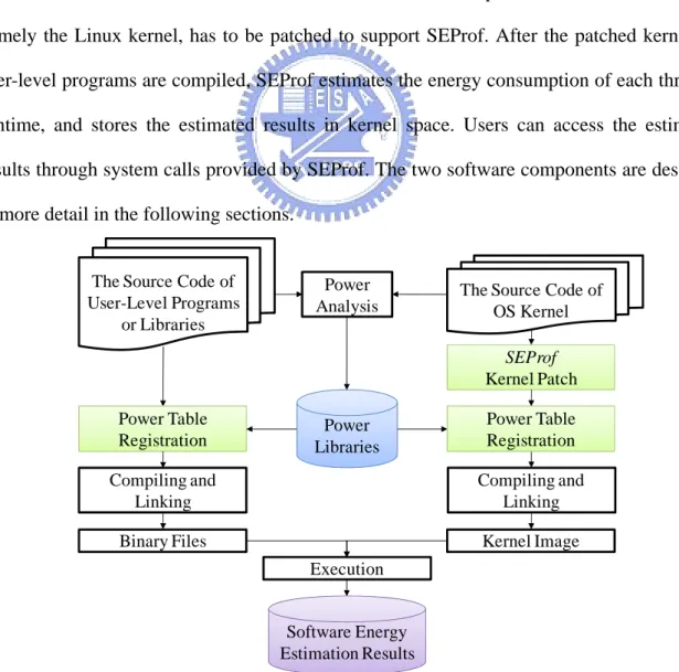
The proposed high-level software energy profiling tool, SEProf, is consisted of two software components, (1) power table registrations and (2) a kernel patch. As depicted in Figure 1, before using SEProf, the power consumption of the processor executing the embedded software has to be analyzed by using measurement-based or lower level modeling-based energy estimation tools which have been discussed in Section 2. After building high-level power libraries for embedded software through power analysis, these power libraries have to be inserted into embedded software, and registered through system calls provided by SEProf for energy estimation at runtime. In SEProf, the energy consumption of embedded software is calculated and maintained in kernel space, therefore the OS kernel, namely the Linux kernel, has to be patched to support SEProf. After the patched kernel and user-level programs are compiled, SEProf estimates the energy consumption of each thread at runtime, and stores the estimated results in kernel space. Users can access the estimation results through system calls provided by SEProf. The two software components are described in more detail in the following sections.
Figure 1. Overview of SEProf
The Source Code of User-Level Programs or Libraries Power Table Registration Compiling and Linking Binary Files
The Source Code of OS Kernel Kernel Image Execution Software Energy Estimation Results Power Libraries Compiling and Linking Power Analysis SEProf Kernel Patch Power Table Registration
3.1. Power Table Registration
By using high-level power modeling techniques, users of SEProf have to build power libraries for embedded software as a reference of the average power consumption of the executing embedded software. A power library is consisted of one or more power tables, and each power table records a number of average power consumptions that an embedded processor executes a specific sequence of instructions, e.g. a basic-block, a function, or a program. The number of average power consumptions recorded in a power table is determined by the number of configurable power levels supported by the embedded processor. For example, a power table may record five different average power consumptions of a specific function executed by an embedded processor which supports up to five different power levels.
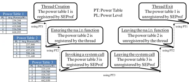
After building power libraries, users have to register and unregister power tables in embedded software through system calls provided by SEProf. This procedure is called “power table registration” as shown in Figure 1. A power table registering operation has to be coupled with an unregistering operation. If a power table is registered to SEProf, it will be used by SEProf as the source of the average power consumption of the executing software. On the contrary, if a power table is unregistered to SEProf, then the power table will no longer be used to estimate the power consumption. An example of using power tables is depicted in Figure 2. It is an execution flow of an example program. We assume that the embedded processor which executes this example program supports up to five different power levels. Therefore, each power table records five average power consumptions of the embedded processor operating at different power levels. In this example, three power tables are built by users, and the features of the three power tables are described as follows. The power table 1 records the average power of all programs on the system. It is registered when a thread is created, and unregistered when a thread is terminated. The power table 2 records the average
Figure 2. An example of using power tables
power of the example program. It is registered at the beginning of the main function in the example program, and unregistered at the end of it. The power table 3 records the average power of all system calls. It is registered at the beginning of the system call handler in OS kernel, and unregistered at the end of it. As shown in Figure 2, when a thread which executes the example program is created, SEProf registers the power table 1 for it in OS kernel. If there is no other power table registered afterwards, the power table 1 will be used as the source of the average power consumption throughout the execution of the thread until the power table 1 is unregistered. However, in this example, the thread registers the power table 2 after entering the main function of the example program. Therefore, the power table 2 becomes the source of the average power consumption of the thread after registration. To further improve the accuracy of power estimation, users in this example also build a power table for system calls, i.e. the power table 3. Hence, every time the thread invokes a system call, the power table 3 is used to estimate the power consumption of the thread, and the power table 2 is used again only when the thread returns from the system call.
3.2. Energy Estimation
When the OS kernel and user-level programs with power table registered are executing,
Power Table 1 PL Avg. Power(uW) 1 236,264 2 319,704 3 419,068 4 536,584
5 668,093 Entering the main function
The power table 2 is registered by the thread Thread Creation
The power table 1 is registered by SEProf
Thread Exit The power table 1 is unregistered by SEProf Leaving the main function
The power table 2 is unregistered by the thread Invoking a system call
The power table 3 is registered by SEProf
Leaving the system call The power table 3 is unregistered by SEProf using PT1 using PT1 using PT2 using PT3 using PT2 Power Table 2 PL Avg. Power(uW) 1 257,860 2 349,031 3 457,676 4 586,146 5 731,460 Power Table 3 PL Avg. Power(uW) 1 235,219 2 318,705 3 416,343 4 529,410 5 662,030 PT: Power Table PL: Power Level
SEProf calculates the energy consumption of each thread by the following formula
∑
= × = N i i i i thread T PT PL CID E 1 )] ( [ (1)where Ethread is the energy consumption of a thread, N is the number of runtime periods of a
thread, Ti is the execution time of the thread in the ith runtime period, CIDi is the
identification (ID) of the embedded processor core executing the thread in the ith runtime period, PL(CIDi) is the power level of the processor core whose ID is CIDi, PTi is the power
table used in the ith runtime period, and PTi[PL(CIDi)] is the average power in the ith runtime
period. A runtime period used in formula (1) is a period of time in the execution time of a thread. In SEProf, a runtime period of a thread is divided and used to estimate the energy consumption of the thread when one of the following four events occurs.
(1) A thread registers or unregisters a power table.
When a thread registers or unregisters a power table, it means that the average power consumption of the embedded processor is changed. Therefore, the average power consumption stored in the previous power table is used to estimate the energy consumption during the former runtime period, and the new power table is applied to the latter periods.
(2) The power level of the embedded processor which executes a thread is changed.
When the power level of an embedded processor is changed, the power consumption of the processor which executes the thread is also changed. Hence, the previous power level is used to estimate the energy consumption during the former runtime period, and the new power level is applied to the following periods.
(3) The total energy consumption of a thread is retrieved while the thread is running.
Before returning the total energy consumption of the thread to users, SEProf adds the energy consumption of the thread since it was last calculated to the total energy consumption of the thread.
(4) A thread is dead.
When a thread is dead, the energy consumption of the thread since it was last calculated is added to the total energy consumption of the thread.
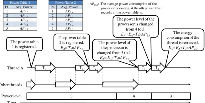
An example of the energy estimation in SEProf using formula (1) is given in Figure 3. We assume that a thread, “Thread A,” executes the same example program as described in Figure 2, and the thread is executed on a single-core embedded processor which supports up to five different power levels. At the beginning of this example, the power level of the embedded processor is set to 5, and the power table 1 is registered for the newly created thread. In Figure 3 the energy consumption of the thread is calculated four times due to three of the above mentioned events. At the end of the runtime period T1 the thread resisters the power table 2 as
the source of the average power consumption. Therefore, the power table 1 is used to calculate the energy consumption during the runtime period T1, and the power table 2 is used
in the following runtime periods. At the beginning of the runtime period T3, SEProf notices
that the power level of the processor has been changed since the thread is scheduled out at the end of the runtime period T2. Hence, it calculates the energy consumption of the thread during
Figure 3. An example of the energy estimation in SEProf
Power Table 1 PL Avg. Power 1 AP1,1 2 AP1,2 3 AP1,3 4 AP1,4 5 AP1,5 T1 Time Thread A Other threads Power level 5 The power table
1 is registered.
T1 T2
3 T3
The power table 2 is registered.
EA= T1×AP1,5
T4
The power level of the processor is changed
from 4 to 3.
EA= EA+T3×AP2,4 The energy
consumption of the thread is retrieved. EA= EA+T4×AP2,3 Power Table 2 PL Avg. Power 1 AP2,1 2 AP2,2 3 AP2,3 4 AP2,4 5 AP2,5
The power level of the processor is changed from 5 to 4.
EA= EA+T2×AP2,5
APm,n: The average power consumption of the
processor operating at the nth power level records in the power table m.
the runtime period T2 using the recorded power level, and updates the recorded power level to
the new one. A similar situation happens at the end of the runtime period T3, but this time the
power level of the processor is changed by “Thread A” itself. In this example, the total energy consumption of “Thread A” retrieved at the end of the runtime period T4 is EA=(T1×AP1,5)+
(T2×AP2,5)+ (T3×AP2,4)+ (T4×AP2,3).
3.3. Data Structures
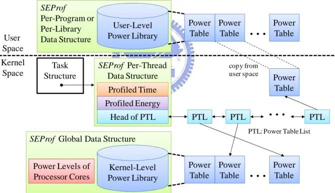
To support thread-based energy estimation, SEProf maintains three kinds of data structures as depicted in Figure 4. They are described as follows:
(1) A per-program/per-library data structure in user space.
It contains a user-level power library which is built from the power analysis of a user-level program/library and stored in the program/library. A user-level power library is consisted of one or more user-level power tables which are used by all threads running the same program/library.
(2) A global data structure in kernel space.
It contains a kernel-level power library, and variables used to record the power levels of all embedded processor cores on the system. The kernel-level power library is built from the power analysis of OS kernel, and stored in the kernel image. A kernel-level power library is consisted of one or more kernel-level power tables which are shared among all threads on the system.
(3) A per-thread data structure in kernel space.
It contains the profiled time and energy of a thread, and a power table list for tracking all registered power tables of the thread. It also records the ID and the power level of the processor core which executes the thread previously for detecting changes of the average power consumption which has been discussed in Section 3.2.
registers a kernel-level power table to SEProf, a new element which points to the registered power table is inserted into the power table list of the thread. When a user-level power table is registered, the content of the registered power table is copied from user space to kernel space first, and a new element which points to the power table in kernel space is inserted into the power table list of the thread. The latest inserted element in the power table list is the one used to estimate the power consumption of the executing thread. In contrast to register a power table, if a power table of a thread is unregistered, the latest registered element will be removed from the power table list of the thread, and the previous registered power table will be used to estimate the power consumption of the executing thread.
Figure 4. Data structures maintained by SEProf
SEProf
Per-Program or Per-Library Data Structure
SEProf Global Data Structure Task Structure SEProf Per-Thread Data Structure Profiled Time Profiled Energy Power Table Kernel-Level Power Library Power Table Power Table
…
PTL: Power Table List
Head of PTL PTL PTL
…
PTL Power Levels of Processor Cores Power Table User-Level Power Library Power Table Power Table…
User Space Kernel Space Power Table copy from user space4. Case Study: ARM11 MPCore Processor
To demonstrate the feasibility of SEPorf, SEProf was adopted to estimate the energy consumption of embedded software executing on an ARM11 MPCore processor [15]. Experimental environment and results are described in Section 4.1 and Section 4.2 respectively.
4.1. Experimental Environment
The experimental platform is a Core Tile, CT11MPCore [16], which has an ARM11 MPCore test chip that implements the ARM11 MPCore processor stacked on the top of a RealView Emulation Baseboard [17]. As shown in Figure 5, the ARM11 MPCore processor is a multi-core processor which supports up to four MP11 central processing units (CPUs). Each MP11 CPU has 16KB-64KB independent data cache and instruction cache. The coherence among data caches of MP11 CPUs is maintained by a snoop control unit (SCU) in the processor. A unified 1 MB L2 cache and the ARM11 MPCore processor are implemented on the ARM11 MPCore test chip. On this platform, all MP11 CPUs on the ARM11 MPCore processor has the same power supply and clock source. The voltage level of the ARM11
Figure 5. Overview of the ARM11 MPCore Processor
CT11MPCore
ARM11 MPCore Test Chip ARM11 MPCore Processor
L2 Cache Controller Snoop Control Unit (SCU) MP11 CPU I D MP11 CPU I D MP11 CPU I D MP11 CPU I D Power Supply Unit
DAC ADC
VDDCORE
PLL
CLK
MPCore processor could be changed by writing values to a digital to analog converter (DAC) on the CT11MPCore, and the voltage and current values of the processor are able to be obtained from an analog to digital converter (ADC). By default, the voltage supplied to the ARM11 MPCore processor is 1.2 V which has an adjustment range of ±0.25V. The clock rate of the processor could also be changed by configuring the phase-locked loop (PLL) on the CT11MPCore. In the experiments, the DAC and PLL were used to scale the voltage and the frequency of the ARM11 MPCore processor respectively, and the ADC was used to measure the power consumption of the processor. For time measurement, a 24 MHz clock on the Emulation Baseboard was used. The time resolution is around 41.7 ns.
In the experiments, SEProf was integrated into Linux kernel 2.6.19, and a patched OProfile [19] was adopted to build power libraries and verify the accuracy of the power estimation results. OProfile is a system-wide profiler for Linux systems using statistical sampling. It could be used to profile Linux kernel, shared libraries, and applications. Originally, OProfile samples the context and program counter (PC) value of the running task on each sampling interrupt, but we extended it to sample the power consumption of the processor as well. We set the sampling rate of OProfile to 1 kHz, and assumed that a power sample could represent the average power consumption of the sampling period.
There are four testing programs used throughout the experiments. Three of them are CG, FT, and IS applications from the OpenMP Implementation of NAS Parallel Benchmarks (NPB) (Version 3.3) [20]. CG computes an approximation to the smallest eigenvalue of a matrix using a conjugate gradient method, FT performs the time integration of a three-dimensional partial differential equation using the Fast Fourier Transform, and IS sorts integers using the bucket sort. The last one testing program, FileRW, is an I/O intensive application which is written by us. It is a simple application which writes and reads a 30,000,000 bytes file on the file system mounted via network file system (NFS).
4.2. Experimental Results
Since we did not successfully scale the frequency of the ARM11 MPCore processor without resetting it, the experiments were separated into two parts. The first one was voltage and frequency scaling (VFS) experiment, and the second one was dynamic voltage scaling (DVS) experiment. In VFS experiment, both of the voltage and the frequency of the ARM11 MPCore processor were scaled at the beginning of the experiment and remained the same throughout the experiment. In DVS experiment, only the voltage of the ARM11 MPCore processor was scaled dynamically and periodically.
4.2.1. VFS Experiment
In VFS experiment, we selected five power levels for the ARM11 MPCore processor, and assumed that the processor only operated at one of the five power levels during the experiment. As shown in Table 1, each power level represents a combination of the voltage and the frequency levels of the processor. In the power analysis stage, only one MP11 CPU was active during the experiment in order to map the measured power consumption back to the embedded software. The remaining three CPUs were not initialized. After analyzing the power consumption of the embedded software using the patched OProfile, we built seven power libraries which are shown in Table 2 for six applications and the Linux kernel, since they took almost all CPU time during the experiment. Each power library only contains one power table, and each power table is consisted of five average power consumptions. The user-level power tables of the six applications are registered to SEProf at the beginning of the applications, and unregistered at the end of it. A kernel-level power table for the Linux kernel, “vmlinux,” is registered to SEProf when a thread is created, and unregistered when the thread is dead. It is also registered when a thread calls a system call, and unregistered when the thread returns from the system call. After building and registering power tables, the applications and the Linux kernel have to be re-compiled. While they are in execution, SEProf
uses the registered power tables to estimate their energy consumption.
The energy estimation results of the testing programs generated by SEProf are depicted in Table 3. The energy and time spent on executing application itself and calling system calls are separated for better examining the accuracy of the power estimation results. In Table 3, it can be observed that in many cases the average power consumption which belongs to the application itself is slightly lower than the average power consumption recorded in Table 2. This is because the power table “vmlinux” which has lower average power consumption than
Table 1. Power levels of the ARM11 MPCore processor used in VFS experiment
Power Level Voltage (V) Frequency (MHz)
1 0.95 140
2 1.01 168
3 1.08 196
4 1.14 224
5 1.2 252
Table 2. Pre-built power tables used in VFS experiment
Power Level
Average Power (uW)
busybox cg.W ft.W is.W FileRW oprofiled vmlinux 1 259,910 248,793 257,860 245,596 245,596 263,693 236,264
2 351,942 335,212 349,031 333,724 329,615 359,267 319,704
3 460,445 438,194 457,676 437,932 430,954 469,998 419,068
4 589,110 558,713 586,146 560,148 565,448 602,413 536,584
5 737,875 696,401 731,460 700,672 692,258 753,294 668,093
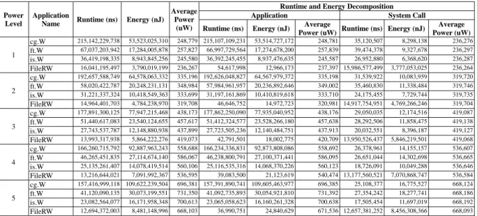
Table 3. Energy estimation results of the testing programs generated by SEProf
Power Level
Application
Name Runtime (ns) Energy (nJ) Average
Power (uW)
Runtime and Energy Decomposition
Application System Call Runtime (ns) Energy (nJ) Average
Power (uW) Runtime (ns) Energy (nJ)
Average Power (uW) 1 cg.W 215,142,229,738 53,523,025,310 248,779 215,107,109,231 53,514,727,172 248,781 35,120,507 8,298,138 236,276 ft.W 67,037,203,942 17,284,005,878 257,827 66,997,729,564 17,274,678,200 257,839 39,474,378 9,327,678 236,297 is.W 36,419,198,335 8,943,845,256 245,580 36,392,245,455 8,937,476,635 245,587 26,952,880 6,368,620 236,287 FileRW 16,041,195,497 3,790,019,199 236,267 54,617,998 12,966,173 237,397 15,986,577,499 3,777,053,025 236,264 2 cg.W 192,657,588,749 64,578,063,332 335,196 192,626,048,827 64,567,979,372 335,198 31,539,922 10,083,959 319,720 ft.W 58,020,422,787 20,248,231,131 348,984 57,984,961,957 20,236,892,646 349,002 35,460,830 11,338,484 319,746 is.W 31,221,337,324 10,418,549,363 333,699 31,197,161,869 10,410,819,618 333,710 24,175,455 7,729,744 319,735 FileRW 14,964,401,703 4,784,238,970 319,708 46,646,752 14,972,723 320,981 14,917,754,951 4,769,266,246 319,704 3 cg.W 177,891,300,125 77,947,215,468 438,173 177,862,250,090 77,935,040,952 438,176 29,050,035 12,174,516 419,087 ft.W 51,440,617,083 23,540,124,655 457,617 51,412,324,577 23,528,266,180 457,638 28,292,506 11,858,475 419,138 is.W 27,743,537,787 12,148,880,938 437,899 27,723,505,236 12,140,484,751 437,913 20,032,551 8,396,187 419,127 FileRW 13,993,317,938 5,864,222,276 419,073 42,791,501 18,002,775 420,709 13,950,526,437 5,846,219,501 419,068 4 cg.W 166,260,715,792 92,887,963,243 558,688 166,234,336,831 92,873,808,086 558,692 26,378,961 14,155,157 536,607 ft.W 46,265,451,835 27,114,674,140 586,067 46,238,800,791 27,100,371,441 586,095 26,651,044 14,302,698 536,665 is.W 25,135,261,407 14,078,419,514 560,106 25,116,535,316 14,068,370,226 560,123 18,726,091 10,049,288 536,646 FileRW 13,216,644,021 7,091,992,367 536,595 39,083,500 21,123,619 540,474 13,177,560,521 7,070,868,747 536,584 5 cg.W 157,416,999,118 109,622,239,504 696,381 157,391,890,741 109,605,463,977 696,385 25,108,377 16,775,527 668,124 ft.W 41,120,090,135 30,073,199,551 731,350 41,092,735,893 30,054,921,810 731,392 27,354,242 18,277,741 668,186 is.W 23,082,564,077 16,171,958,348 700,613 23,065,058,623 16,160,261,328 700,638 17,505,454 11,697,019 668,192 FileRW 12,694,372,003 8,481,148,996 668,103 36,990,751 24,840,629 671,536 12,657,381,252 8,456,308,366 668,093
other power tables is used to estimate the power consumption of an application when its own power tables is not registered. Another observation in Table 3 is that the average power consumption of a thread calling system calls is slightly higher than the average power recorded in the power table “vmlinux.” The reason is that the power table “vmlinux” is used for all system calls except the one for registering/unregistering a power table to avoid removing the newly registered power table when a thread returns from the system call. Therefore, the average power consumption of a thread calling system calls is slightly increased every time the system call for registering/unregistering a power table is called during the experiment.
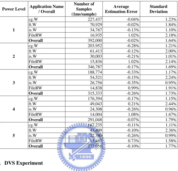
The accuracy of the power estimation results shown in Table 3 is verified in Table 4. We patched OProfile to sample the measured power and the estimated power on each sampling interrupt, and compared their values to calculate the power estimation error. As shown in Table 4, we examined the power estimation error of the four testing programs, and we also examined the power estimation error of an overall period which began when the init process executed the programs in the appropriate rc directory and ended when the last testing program was finished. The power estimation error of the overall period could represent that of partial Linux kernel and many applications executed during the period. Based on the results shown in Table 4, it can be seen that the power estimation error using SEProf is quite low. In most cases, the average estimation error is less than 2% and the standard deviation of the estimation error is less than 3%.
Table 4. Power estimation error in VFS experiment
Power Level Application Name / Overall Number of Samples (1ms/sample) Average Estimation Error Standard Deviation 1 cg.W 227,437 -0.04% 1.23% ft.W 70,929 -0.02% 1.84% is.W 34,767 -0.13% 1.10% FileRW 16,935 1.02% 2.18% Overall 392,000 -0.02% 1.64% 2 cg.W 203,952 -0.28% 1.21% ft.W 61,413 -0.12% 2.00% is.W 30,003 -0.21% 1.01% FileRW 15,836 1.02% 2.14% Overall 346,787 -0.17% 1.69% 3 cg.W 188,774 -0.33% 1.17% ft.W 54,521 -0.15% 2.24% is.W 26,756 -0.35% 0.95% FileRW 14,838 0.99% 1.91% Overall 315,333 -0.26% 1.73% 4 cg.W 176,394 -0.17% 1.15% ft.W 49,043 0.21% 2.44% is.W 24,308 -0.26% 0.96% FileRW 14,004 1.08% 1.67% Overall 291,048 -0.07% 1.79% 5 cg.W 167,235 -0.11% 1.11% ft.W 43,609 -0.10% 2.36% is.W 22,380 -0.26% 0.99% FileRW 13,467 0.73% 1.58% Overall 272,056 -0.10% 1.77% 4.2.2. DVS Experiment
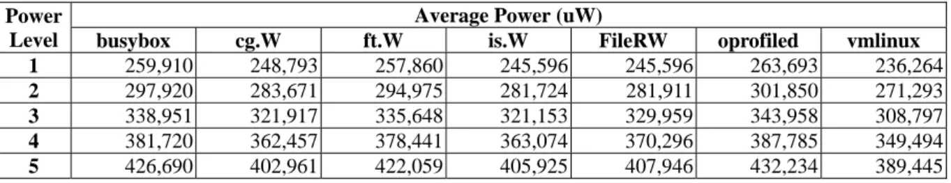
The primary difference between SEProf and the existing high-level modeling-based software energy estimation tools is that SEProf is aware of the changes in the power levels of embedded processors at runtime. This feature is examined in this section. As in VFS experiment, we selected five power levels for the ARM11 MPCore processor, but in DVS experiment the clock frequency of the processor operating at each power level is the same as shown in Table 5, since we did not successfully scale the frequency of the processor without resetting it. Nevertheless, it does not prevent us from examining that SEProf supports the above mentioned feature, because the power consumption of the processor is also dynamically changed by scaling the voltage of the processor at runtime. In DVS experiment, as in VFS experiment, only one MP11 CPU was active, and seven power tables were built for the six applications and the Linux kernel as shown in Table 6.
Table 5. Power levels of the ARM11 MPCore processor used in DVS experiment
Power Level Voltage (V) Frequency (MHz)
1 0.95 140
2 1.01 140
3 1.08 140
4 1.14 140
5 1.2 140
Table 6. Pre-built power tables used in DVS experiment
Power Level
Average Power (uW)
busybox cg.W ft.W is.W FileRW oprofiled vmlinux 1 259,910 248,793 257,860 245,596 245,596 263,693 236,264
2 297,920 283,671 294,975 281,724 281,911 301,850 271,293
3 338,951 321,917 335,648 321,153 329,959 343,958 308,797
4 381,720 362,457 378,441 363,074 370,296 387,785 349,494
5 426,690 402,961 422,059 405,925 407,946 432,234 389,445
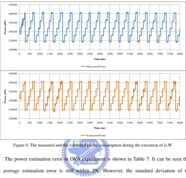
In DVS experiment, the voltage of the processor was periodically scaled at three different time intervals, 100 ms, 1 s, and 10 s. At each time interval, the power level of the processor was increased by one. If the power level of the processor reached to five, then it was set to one at the next time interval. An example of DVS experiment is depicted in Figure 6. In the figure, two lines show the measured and the estimated power consumption of the processor sampled by the patched OProfile during the execution of the IS application. The DVS interval was set to 100 ms in this example, therefore the power consumption of the processor was varied every 100 ms. It can be seen in Figure 6 that the estimated power consumption is very close to the measured one. However, sometimes the line of the estimated power consumption is dropped but that of the measured one is not. This is because that the thread which executed the IS application was scheduled out during that period, and another thread which used a different power table was scheduled in. If the newly scheduled thread had lower average power consumption, then a drop will be displayed in the figure. On the other hand, for the line of the measured power consumption, since the time interval that the power consumption read from ADC is updated around every 5 ms, the power drop will not be shown in Figure 6 if the newly scheduled thread is scheduled out immediately within the update period of the ADC.
Figure 6. The measured and the estimated power consumption during the execution of is.W
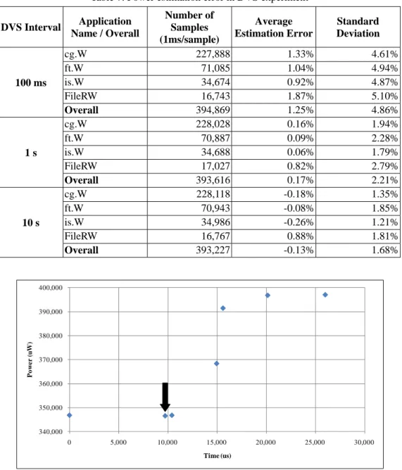
The power estimation error in DVS experiment is shown in Table 7. It can be seen that the average estimation error is still within 2%. However, the standard deviation of the estimation error becomes larger with the decreasing DVS interval. It is because the power consumption of the processor is not changed immediately after a new value is written to the DAC, and the changed power consumption of the processor is not able to be read from the ADC immediately. We explain this in Figure 7 which draws seven power samples taken from the ADC during the period that the voltage level of the processor is scaling. An arrow in Figure 7 indicates the time that the new voltage level is written to the DAC. SEProf updates the power level of the processor at this point. Nevertheless, the power consumption of the processor does not be changed immediately. Instead, it becomes stable and able to be read form ADC in the next 10 ms. Consequently, the power consumption difference between the measured and the estimated ones during this period enlarges the standard deviation of the estimation error. 200000 250000 300000 350000 400000 450000 0 500 1000 1500 2000 2500 3000 3500 4000 4500 5000 5500 6000 6500 7000 7500 8000 Po w e r ( u W ) Time (ms)
Mea sured Power
200000 250000 300000 350000 400000 450000 0 500 1000 1500 2000 2500 3000 3500 4000 4500 5000 5500 6000 6500 7000 7500 8000 P o w er ( u W ) Time (ms)
Table 7. Power estimation error in DVS experiment DVS Interval Application Name / Overall Number of Samples (1ms/sample) Average Estimation Error Standard Deviation 100 ms cg.W 227,888 1.33% 4.61% ft.W 71,085 1.04% 4.94% is.W 34,674 0.92% 4.87% FileRW 16,743 1.87% 5.10% Overall 394,869 1.25% 4.86% 1 s cg.W 228,028 0.16% 1.94% ft.W 70,887 0.09% 2.28% is.W 34,688 0.06% 1.79% FileRW 17,027 0.82% 2.79% Overall 393,616 0.17% 2.21% 10 s cg.W 228,118 -0.18% 1.35% ft.W 70,943 -0.08% 1.85% is.W 34,986 -0.26% 1.21% FileRW 16,767 0.88% 1.81% Overall 393,227 -0.13% 1.68%
Figure 7. Power samples during DVS
In the last experiment, we measured the performance overhead introduced by using SEProf in DVS experiment. As shown in Table 8, two types of SEProf were implemented and evaluated. The first type of SEProf is called “SEProf - Time Only”. It only profiled time information of all threads at runtime, and was used to examine the performance overhead caused by profiling time information. The second type of SEprof is called “SEProf” in Table 8. It profiled both time and energy of all threads at runtime. Table 8 listed the length of the two time periods that the testing programs ran under the Linux kernels patched by the two types of
340,000 350,000 360,000 370,000 380,000 390,000 400,000 0 5,000 10,000 15,000 20,000 25,000 30,000 P o w er ( u W ) Time (us)
SEProf. These two time periods were normalized to the length of the time period that the testing programs ran under an unmodified Linux kernel. In Table 8, it can be seen that the overhead of using SEProf is less than 1% which is quite small even when the DVS interval is 100 ms.
Table 8. Performance overhead of using SEProf in DVS experiment
DVS Interval Application Name / Overall
SEProf –
Time Only SEProf
100 ms cg.W 0.33% 0.22% ft.W -0.96% -0.15% is.W 0.15% 0.98% FileRW 0.68% 0.54% Overall 0.10% 0.26% 1 s cg.W 0.09% 0.29% ft.W -0.11% 0.04% is.W -0.07% -0.04% FileRW -1.02% -1.26% Overall -0.05% 0.08% 10 s cg.W -0.85% -1.01% ft.W 0.92% -0.14% is.W -2.34% -0.32% FileRW -0.35% -0.39% Overall -0.62% -0.71%
5. Conclusions and Future Works
In this paper, a high-level modeling-based software energy profiling tool, SEProf, was proposed and implemented. SEProf estimates the energy consumption of each thread by maintaining a power table list for each thread and tracking the power levels of embedded processors at runtime which makes SEProf more suitable for energy estimation on larger systems with power management enabled. We implemented SEProf in Linux kernel 2.6.19, and conducted a number of experiments on an ARM11 MPCore processor. The experimental results in VFS experiment show that the average power estimation error using SEProf is within 2% and the standard deviation of the estimation error is within 3%. The results in DVS experiment indicate that the average power estimation error is within 2%, but the standard deviation of the estimation error becomes larger with the decreasing DVS interval. The performance overhead introduced by SEProf is quite less. The observed performance degradation in DVS experiment is less than 1%. Users of SEProf could control the trade-off between accuracy and efficiency by building power libraries for embedded software at various granularity levels.
Currently, users of SEProf have to register/unregister power tables and insert probes to retrieve the estimated energy consumption of threads in the source code of embedded software manually and carefully. It is not very convenience for users and not applicable if the source code of embedded software is not available. We consider adopting dynamic instrumentation technique, such as techniques used in DTrace [21] or Pin [22], in the future to overcome this shortcoming. Furthermore, a systematic method to choose and build power tables would also be one of the future works.
References
[1] K. Choi, R. Soma, and M. Pedram, "Fine-Grained Dynamic Voltage and Frequency Scaling for Precise Energy and Performance Tradeoff Based on the Ratio of Off-Chip Access to On-Chip Computation Times," IEEE Transactions on Computer-Aided Design of Integrated Circuits and Systems, vol. 24, NO. 1, January 2005.
[2] C. Isci, A. Buyuktosunoglu, C.-Y. Cher, P. Bose, and M. Martonosi, "An Analysis of Efficient Multi-Core Global Power Management Policies: Maximizing Performance for a Given Power Budget, " the 39th Annual IEEE/ACM International Symposium on Microarchitecture (MICRO), 2006.
[3] J. Flinn and M. Satyanarayanan, "PowerScope: A Tool for Profiling the Energy Usage of Mobile Applications," in Proceedings of the Second IEEE Workshop on Mobile Computer Systems and Applications (WMCSA), 1999.
[4] D. Brooks, V. Tiwari, and M. Martonosi, "Wattch: A Framework for Architectural-Level Power Analysis and Optimizations," 27th International Symposium on Computer Architecture (ISCA-27), June 2000.
[5] M. Monchiero, R. Canal, and A. Gonzalez, "Power/Performance/Thermal Design-Space Exploration for Multicore Architectures," IEEE Transactions on Parallel and Distributed Systems, Vol. 19, No. 5, May 2008.
[6] V. Tiwari, S. Malik, and A. Wolfe, "Power analysis of embedded software: A first step towards software power minimization," IEEE Transactions on Very Large Scale Integration (VLSI) Systems, Vol. 2, Issue 4, pp. 437-445, Dec. 1994.
[7] A. Sinha and A. P. Chandrakasan, "Jouletrack - a web based tool for software energy profiling," in Proceedings of the Design Automation Conference (DAC), 2001.
[8] H. Blume, D. Becker, L. Rotenberg, M. Botteck, J. Brakensiek, and T.G. Noll, "Hybrid functional- and instruction-level power modeling for embedded and heterogeneous
processor architectures," Journal of Systems Architecture, Vol. 53, Issue 10, pp. 689–702, 2007.
[9] H. Blume, J.v. Livonius, L. Rotenberg, T.G. Noll, H. Bothe, and J. Brakensiek, "Performance and Power Analysis of Parallelized Implementations on an MPCore Multiprocessor Platform," International Conference on Embedded Computer Systems: Architectures, Modeling and Simulation (IC-SAMOS), 2007.
[10] T. K. Tan, A. Raghunathan, and N. K. Jha, "EMSIM: An energy simulation framework for an embedded operating system," in Proceedings of IEEE International Symposium on Circuit & Systems, pages 464–467, May 2002.
[11] T. K. Tan, A. Raghunathan, and N. K. Jha, "A simulation framework for energy consumption analysis of OS-driven embedded applications," IEEE Transactions on Computer-Aided Design of Integrated Circuits and Systems, 22(9) 1284-1294, Sept. 2003.
[12] T. K. Tan, A. Raghunathan, G. Lakshminarayana, and N. K. Jha. "High-level software energy macro-modeling," in Proceedings of Design Automation Conference, June 2001. [13] G. Qu, N. Kawabe, K. Usami, and M. Potkonjak, “Function-level power estimation
methodology for microprocessors,”in Proceedings of Design Automation Conference (DAC), pp. 810–813, 2000.
[14] C.-H. Hsu, J.-J. Chen, and S.-L. Tsao, "Evaluation and Modeling of Power Consumption of a Heterogeneous Dual-Core Processor," in the 13th International Conference on Parallel and Distributed Systems (ICPADS), Hsinchu, Taiwan, Dec. 2007.
[15] "ARM11 MPCore Processor Revision r1p0 Technical Reference Manual," ARM, Feb. 2008.
[16] "Core Tile for ARM11 MPCore HBI-0146 User Guide," ARM, September 2006. [17] "RealView™ Emulation Baseboard HBI-0140 Rev D User Guide," ARM, Oct. 2007. [18] R. Kumar, K. I. Farkas, N. P. Jouppi, P. Ranganathan, and D. M. Tullsen, "Single-ISA
Heterogeneous Multi-Core Architectures: The Potential for Processor Power Reduction," in Proceedings of the 36th International Symposium on Microarchitecture (MICRO), Dec. 2003.
[19] J. Levon, "OProfile Internals," http://oprofile.sourceforge.net/doc/internals/index.html, 2003.
[20] H. Jin, M. Frumkin, and J. Yan, "The OpenMP Implementation of NAS Parallel Benchmarks and Its Performance," NAS Technical Report NAS-99-011, NASA Ames Research Center, Oct. 1999.
[21] B. M. Cantrill, M. W. Shapiro, and A. H. Leventhal, "Dynamic Instrumentation of Production Systems," in Proceedings of the 2004 USENIX Annual Technical Conference, Boston, MA, USA, 2004.
[22] C.-K. Luk, R. Cohn, R. Muth, H. Patil, A. Klauser, G. Lowney, S. Wallace, V. J. Reddi, K. Hazelwood, "Pin: building customized program analysis tools with dynamic instrumentation," in Proceedings of the ACM SIGPLAN conference on Programming language design and implementation (PLDI), pp. 190 - 200, 2005.