管理浮動匯率之探討

行政院國家科學委員會專題研究計畫 成果報告

管理浮動匯率之探討

中 華 民 國 94 年 10 月 13 日

行政院國家科學委員會專題研究計劃成果報告

管理浮動匯率之探討

Characterize the Managed Floating Exchange Rates

1

Introduction

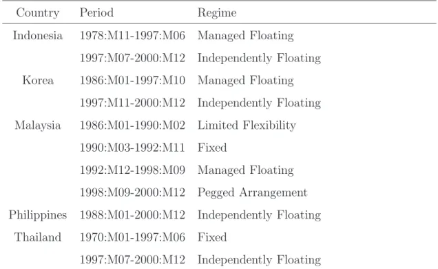
As international capital markets are becoming more integrated, a currently fashionable view of choosing exchange rate regimes is that countries are being pushed to the corner: they must choose between either a free floating or a firm fixing regime. People refer to this bipolar proposition as the vanishing intermediate regime, or the missing middle. It is argued that the Asian 1997 currency crisis has supported this proposition, since most Asian countries that suffered the currency crisis adopted the free floating regime (e.g. Indonesia, Korea, the Philippines and Thailand) or a hard peg (Malaysia) after the crisis. According to the official IMF classifications of exchange rate regimes (see Table 1), it is clear that three countries (Indonesia, Korea, and Thailand) have transferred their officially-declared exchange rate regimes into more flexible ones due to the crisis , while Malaysia moved in the opposite direction. Only the Philippines retained its pre-crisis free floating exchange rate regime.

Moreover, the “vanishing middle” is also evident in that the intermediate regimes adopted by most countries in the early 1990s are now only used by about one-third of the IMF’s member countries (see Table 2).

Table 1: Official Exchange Rate Regimes in the 1997 Currency Crisis Countries Country Period Regime

Indonesia 1978:M11-1997:M06 Managed Floating 1997:M07-2000:M12 Independently Floating Korea 1986:M01-1997:M10 Managed Floating

1997:M11-2000:M12 Independently Floating Malaysia 1986:M01-1990:M02 Limited Flexibility

1990:M03-1992:M11 Fixed

1992:M12-1998:M09 Managed Floating 1998:M09-2000:M12 Pegged Arrangement Philippines 1988:M01-2000:M12 Independently Floating

Thailand 1970:M01-1997:M06 Fixed

1997:M07-2000:M12 Independently Floating

Source: IMF, Exchange Arrangements and Exchange Restrictions, several issues. Edited by Hern´andez and Montiel (2001).

Table 2: Exchange Rate Arrangements in 1991 and 1999 Hard Pegs Intermediate Floating Year 1991 1999 1991 1999 1991 1999 All Countries 16% 24% 62% 34% 23% 42% Emerging Market Economies 6% 9% 64% 42% 30% 48% Developing and Emerging 5% 25% 65% 27% 29% 47% Market Economies

Source: Fischer (2001). Edited by Bofinger and Wollmershauser (2003).

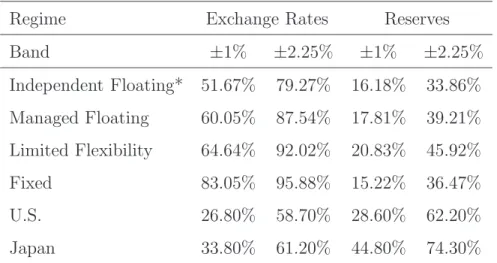
Some observers, however, have noticed that countries that say they allow their ex-change rate to float mostly do not. For instance, Calvo and Reinhart (2002) point out that if a country does follow a pure floating exchange rate policy, the volatility of ex-change rates should be large while the volatility of foreign exex-change reserves should be small (indicating no intervention). They calculate the probability that the monthly per cent changes in nominal exchange rates and foreign exchange reserves fall within a ±1% or

±2.25% band (see Table 3). Using the U.S. and Japan as a benchmark, they find that the average in the countries claiming an independently floating system is far from the bench-mark countries, and is very close to the average of managed floating countries. They denote the findings as “fear of floating,” and they conclude about the Asian countries especially:

“Indeed, once financial markets settled and capital flowed back to Asia, their currencies are fluctuating much the way they did prior to the crisis – that is to say, they are not fluctuating at all.”

Table 3: Main Results of Calvo and Reinhart (2002) Regime Exchange Rates Reserves Band ±1% ±2.25% ±1% ±2.25% Independent Floating* 51.67% 79.27% 16.18% 33.86% Managed Floating 60.05% 87.54% 17.81% 39.21% Limited Flexibility 64.64% 92.02% 20.83% 45.92% Fixed 83.05% 95.88% 15.22% 36.47% U.S. 26.80% 58.70% 28.60% 62.20% Japan 33.80% 61.20% 44.80% 74.30%

(*) Excluding U.S. and Japan. Source: Calvo and Reinhart (2002).

Similarly, using a regression framework adopted from Frankel and Wei (1994) on ex-change rate data of Asian countries from 1999:M1 to 2000:M5, McKinnon (2001) argues:

“In the year 2000, both the crisis and non-crisis countries of East Asia (with Japan remaining the important exception) have returned to formal or informal dollar pegging, which is statistically indistinguishable from what they were doing before the crisis.”

Is the middle disappearing? The answer seems to be no. Most countries adopt so called a managed floating exchange system. Furthermore, official intervention is the most important characteristic of managed floating exchange rates. Due to data unavail-ability, it is always a difficult task for researchers to investigate official intervention in the foreign exchange market. In general, most studies have used changes in foreign reserves

as a proxy for intervention flows. Some researchers consider more variables to measure intervention. They examine changes in nominal exchange rates, foreign reserves, and nominal interest rates. Hence, low volatile exchange rates, high volatile reserves or high variable interest rate may indicate a hid degree of official intervention. See Calvo and Reinhart (2002). These individual measures, however, represent a very inaccurate proxy since there are a number of reasons to the changes of these variables. In many cases, changes in exchange rates, foreign reserves, and nominal interest rates is not caused by official intervention. Moreover, investigating each variable independently may encounter an inconsistent problem since changes in these variables may indicate contradicted results. Weymark (1997) has proposed an alternative approach to measure the degree of ex-change market intervention in a small open economy. By constructing an index of in-tervention activity which is calculated based on observed data, Weymark (1997) uses the index to measure the bilateral and multilateral intervention for Canada over the pe-riod 1975-1990. As commented by Sarno and Taylor (2002), “...Weymark’s measure may represent a plausible alternative to measured changes in international reserves.” This approach is applied in a number of studies,1 _{however, no assessment has yet been made}

on the performance of the Weymark’s measure.

In this paper, we follow the Weymark’s methodology to construct intervention index for Japan in the period from April 1990 to January 2005. We then compare the Weymark’s index with the Japanese public intervention data and assess how well the Weymark’s index performs. The remainder of the paper is as follows. Section 2 provides a brief overview of the Weymark’s measure of intervention. Section 3 describes the data. The empirical results is provided and the robustness issue is discussed in Section 4. Section 5 gives a caveat. Section 6 contains some concluding remarks.

2

Weymark’s Index

Weymark (1997) first presents the following formula for calculating exchange market pres-sure (EMP):

EMPt= ∆et+ η∆rt (1)

1

where et is the logarithm of the exchange rate expressed in terms of the domestic

cur-rency cost of one unit of foreign curcur-rency, ∆et = et− et−1 is the percentage change in the

foreign exchange rate, ∆rt is the percentage change in official foreign reserves expressed

as a proportion of the money base, and η = −∂∆et/∂∆rt, is the elasticity. EMP can be

interpreted as the exchange rate change that would have been required to remove the ex-cess demand for a currency without intervention from the central bank. The intervention index proposed by Weymark (1997) is:

ωt = η∆et EMPt = ∆rt (1/η)∆et+ ∆rt . (2)

It is worthy noting that −∞ < ω < ∞, and the interpretation of ωt is as follows.

1. ω = 0 indicates perfect floating exchange rate regime. 2. ωt= 1 indicates fixed exchange rate regime.

3. 0 < ωt < 1 indicates managed floating exchange rate regime. The degree of

inter-vention is higher when ωt→ 1.

4. ωt> 1 indicates that the central bank actively depreciates (appreciates) the

tic currency with respect to its free float value when the excess demand for domes-tic currency is positive (negative). That is, intervention reverses the exchange rate movement.

5. Finally, ωt < 0 indicates that the central bank undertakes contractionary

interven-tion in response to an excess demand for domestic currency and vice versa.

For the case of managed float, Weymark (1997) notices that 1 > ωt ≥ 0.7 represents a

significant amount of exchange market intervention.

The elasticity η needs to be estimated from a structural model. In this paper we use the same structural model as in Weymark (1997). We will discuss the model specification in Section 5. The details regarding the structural model and estimation strategy are provided in the Appendix.

3

Data and Index

3.1

Data

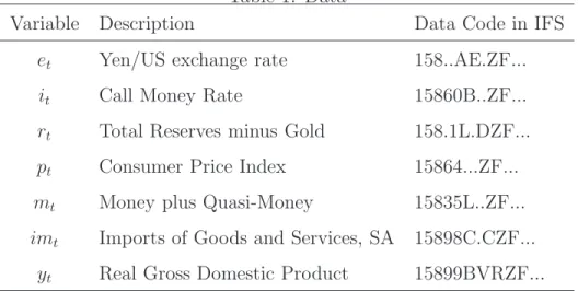
Monthly data for Japan from January 1990 to January 2005 is obtained from IMF’s International Financial Statistics. We match the period with the data of the foreign exchange intervention by choosing 1990 as start date. To construct the Weymark index, we need the following data series. Nominal exchange rate is the bilateral rate of Yen against the US dollar (et = ln(Yen/US dollar)). The call money rate is used as the

domestic interest rate (it). The domestic price level is measured by the consumer price

index. M2 is used as the domestic money stock (mt). Finally, output (yt) is measured

by real GDP. Real GDP is available on quartely basis and we transform the series into monthly basis by the DP algorithm.2

The foreign reserve is the total reserves minus gold. See Table 1 for a detail description of the data series and sources. The results of Augmented Dickey-Fuller test are reported in Table 2. Clearly, all the variables are first difference stationary except for price levels and interest rates.

The official intervention data of Japan is available from the Ministry of Finance web-page (http://www.mof.go.jp/english/e1c021.htm). The historical data, from April 1991 to March 2000, was released in July 2001. Since then the data has been updated: the historical data from April 1991 to June 2005 is available for now. The data includes the following information: (a) the date of intervention, (b) the yen amount and direction (sold/bought) of intervention for the day, (c) currencies that are involved in intervention.

3.2

Index

Since official intervention data is not available in many countries, Weymark (1997) uses the change in foreign reserve (expressed as a proportion of the money base) for ∆rt.

Following Weymark (1997), we construct the index using the change in foreign reserve (expressed as a proportion of the money base) for ∆rt in Japan. We call it the Weymark

index.

2

This is a state-space modelling approach to estimate unobserved high-frequency data. We use the procedure DISTRIB in RATS to produce monthly real GDP. This approach has the feature that the high-frequency data aggregate up to exactly match the low-frequency data.

Notice that the Weymark index is supposed to measure the proportion of exchange market pressure relieved by exchange market intervention. Strictly speaking, however, the Weymark index that uses the change in foreign reserve measures the proportion of exchange market pressure relieved by the change in foreign reserve as a whole, rather than by exchange market intervention alone. Because the change in foreign reserve could be caused not only by exchange market intervention but also by other factors (e.g., the interest earning on Japan’s holding of U.S. bonds), we need to be careful in interpreting the Weymark index as the measure of the proportion of exchange market pressure relieved by exchange market intervention. Fortunately, the data on exchange market intervention is available in Japan. Instead of using the change in foreign reserve, we can construct the “true” Weymark index by using the data on exchange market intervention for ∆rt,

which measures the proportion of exchange market pressure relieved by exchange market intervention alone.3

In next section we compare the Weymark index with the “true” Weymark index.

4

Empirical Results

4.1

A Comparison with Japanese Intervention Data

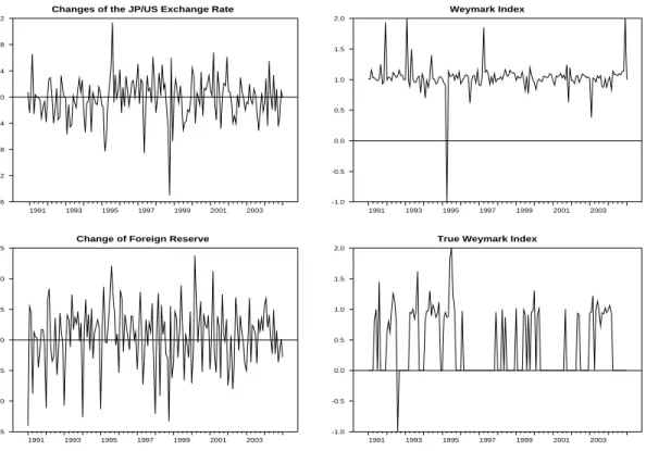
Figure 1 plots the changes in JP/US exchange rates, the change in Japanese foreign reserve, the Weymark index and the true Weymark index. We also report the Weymark index and the true Weymark index in Table 3 and Table 4. Since the index can take extremely large absolute values, we follow Jeisman (2005) to replace extremely large values of the index by 2 when it is larger than 2 and -1 when it is smaller than -1.

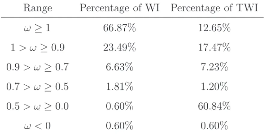
It turns out that the Weymark index and the true Weymark index move very differently in the sample period. The correlation of these two indexes is negative (-0.1875). Table 5 summarizes the distribution of the Weymark index and the true Weymark index for Japan. It is clear that the Weymark index overestimates the degree of intervention in Japan. On the one hand, the Weymark index suggests that Japan has conducted significant intervention in the foreign exchange market: average of the Weymark index is 1.03. On

3

As in construction of the Weymark index, we use the intervention volume expressed as a proportion of the monetary base for ∆rt.

the other hand, the true Weymark index suggests that Japan has not conducted that significant intervention in the foreign exchange market: average of the Weymark index is 0.38. To see the relation between two indexes, we regress the following by OLS.

Weymark Indext = constant + β · True Weymark Indext+ εt (3)

If the Weymark index measures the proportion of exchange market pressure relieved by exchange market intervention precisely, the constant term should be close to zero and β should be close to one. The regression results are summarized in Table 6. The constant term is significantly different from zero. β is significantly negative, which reflects the negative correlation of these two indexes. This means that the Weymark index for Japan does not measure the proportion of exchange market pressure relieved by exchange market intervention very precisely.

Why do these two indexes move so differently? In all months (166 months) during the sample period, the foreign reserve fluctuates irrespective of whether official intervention is actually conducted or not: ∆rt 6= 0 for all t in the Weymark index. As a result, the

Weymark index is always different from zero. Moreover, when the exchange rate does not fluctuate very much (i.e., (1/η)∆et is relatively small in absolute value), the Weymark

index tends to be close to one, even if no intervention is conducted during the period. That is why the Weymark index suggests that Japan has significantly intervened in the foreign exchange market during the sample period. In many months (101 months) during the sample period, however, no intervention was conducted in fact. As a result, the true Weymark index is equal to zero for almost two thirds of the entire sample period. That is, the true Weymark index suggests that Japan has not intervened so often in the foreign exchange market during the sample period. Therefore, according to the comparison of Weymark index and the true Weymark index, it may be concluded that the Weymark index seems not an appropriate measure of intervention activities. Although what we conduct is just a case study, this result may be sufficient to cast a doubt on the usefulness of the Weymark index.

It is worth noting that most intervention activities in Japan are believed to be steril-ized. Weymark (1997) considers the possibility of sterilized intervention and proposes to modify the Weymark index (if necessary) to incorporate sterilized interventions as follows. In order to see the effect of sterilized intervention, a risk premium, δt, is incorporated in

equation (7) of the Appendix.

it= i∗t + E(et+1|Ωt) − et+ δt

Weymark (1997) gives an example when the risk premium δt is endogenous: suppose the

risk premium is endogenous as δt= k∆rtwhere k ∈ [0, 1] represents the fraction of period

t intervention that is sterilized. It can be shown that the sterilized Weymark Index ηs _is

formulated as4

ηs _{= (1 + kb} 2)η.

Hence, the Weymark Index we constructed using η above may underestimate the inter-vention activity when interinter-vention is sterilized (|ηs_{| > |η|). However, notice that if we}

use ηs _{instead of η in the comparison between the Weymark index and the true Weymark}

index, the difference between these two indexes would be larger. Because (1/ηs_)∆e t is

even smaller than (1/η)∆et in absolute value, it is more likely that the Weymark index is

close to one even when the true Weymark index is zero. In other words, the correlation of these two indexes becomes even more negative when we use ηs _{instead of η.}

Weymark (1997) also points out that as long as the risk premium is exogenous (i.e., independent of the policy authority’s choice of ¯ρ in equation (10) of the Appendix), our estimate of η and the resulted Weymark index are appropriate for measuring exchange market pressure and intervention activity when intervention is sterilized. In this case, nothing changes in terms of comparison between the Weymark index and the true Wey-mark index we have conducted above.

In sum, as long as we follow what Weymark (1997) proposes, our results would not change qualitatively even when intervention activities are sterilized. However, it does not necessarily mean that what Weymark (1997) proposes is wrong. We need to be careful in interpreting our results. We will discuss it in Section 5.

4.2

Robustness

In order to check the robustness of the results, we have used alternative measures of some variables to estimate η. We have replaced consumer price index with producer price index (PPI) and GDP deflator (GDPP). The estimated η’s are -11.05 and -9.16 for PPI and

4

GDPP, respectively. We also replace real GDP with industrial production and obtain an estimated ˆη = −10.27. None of these new figures of ˆη alters our main findings.

Furthermore, we use quarterly data to investigate whether data in a lower frequency may change our results. We find that the results are similar to those for the monthly basis. The coefficient on the true Weymark index in equation (3) is again negative, which is insignificant though.5

5

Caveat

We show that the Weymark index and the true Weymark index move very differently in the case of Japan. This may not be surprising if a non-negligible portion of the change in the foreign reserve is caused not by the foreign exchange intervention activities but by other economic movements such as interest receipts on official portfolio holdings, valuation changes on existing reserves and so on. However, it does not necessarily mean that what Weymark (1997) proposes is wrong. On the one hand, if the structural model underlying the Weymark index is correctly specified in the case of Japan, our result may cast a doubt on the usefulness of the Weymark index. On the other hand, if the structural model is misspecified, our result may suggest that we need to choose a structural model underlying the Weymark index very carefully when we apply the Weymark index to different countries. In this section we argue the possibility of misspecification and its implication as a caveat to our results.

What is important in the Weymark index is to estimate η from the structural model. As Weymark (1997) points out, therefore, the calculated index values will always be model-dependent. Weymark (1997) uses the small open economy model for the case of Canada. In this paper we use the same small open economy model for the case of Japan as in Weymark (1997). However, the small open economy model may not be well-suited for explaining Japan. While it is beyond the scope of this paper to find the model correctly specified for Japan, it is worthwhile to point out that a different value of η that might be obtained from other model could lead to different result. To see this, we conduct a simple calibration as follows. We conduct a grid search of η, from -11.0 to -0.01. We generated 100

5

different values of η and then compute the correlation between the Weymark Index and the true Weymark Index.6 _{Then we plot the correlation against η in Figure 2. A threshold}

value of η such the correlation is zero is -0.84123. Therefore, any structural model that yields the estimates η below the threshold value leads to the negative correlation.

The maximum positive correlation is about 0.7245 when η = −0.01. The minimum negative correlation is about -0.1924 when η = −9.1317. It is not surprising that the correlation tends to be larger when η is small in absolute value. When |η| is small, (1/η)∆et is relatively larger in absolute value. As a result, both the Weymark index and

the true Weymark index would be driven mainly by a common component, (1/η)∆et.

That is why the correlation tends to be larger when |η| is small.

This calibration suggests that the accuracy of the Weymark index may depend on the value of η: the correlation between the Weymark index and the true Weymark index could substantially vary across different values of η. Since the value of η is model-dependent, this suggests the importance of the model choice. Even if the Weymark index with the correctly specified structural model is very useful, the misspecification of the structural model could give a picture of intervention activities that is very different from the actual intervention activities. Therefore, we have to choose the structural model very carefully when we apply the Weymark index to different countries.

6

Concluding Remarks

An important issue in the empirical literature on official intervention is the difficulty to obtain official intervention data. Many efforts have been made to estimate unobservable intervention activity. Among numerous measures of official intervention, the index pro-posed by Weymark (1997) is argued to be a plausible measure. In this paper, we construct both the Weymark index and the true Weymark index for Japanese intervention activ-ity. The true Weymark index is computed by plugging in the official intervention data of Japan.

Our result is striking. The correction between the Weymark index and the true Wey-mark index is negative. The WeyWey-mark index suggests a strong intervention of Japanese

6

Results are similar when 1000, or 10000 different values of η are generated. They are available upon request.

monetary authority while the true Weymark index suggests that Japan has not intervened so often in the foreign exchange market during the sample period we investigate. This result may cast a doubt on the usefulness of the Weymark index if the structural model underlying the Weymark index is correctly specified in the case of Japan. If the struc-tural model is misspecified, our result may suggest that we need to choose a strucstruc-tural model underlying the Weymark index very carefully when we apply the Weymark index to different countries.

Table 1: Data

Variable Description Data Code in IFS et Yen/US exchange rate 158..AE.ZF...

it Call Money Rate 15860B..ZF...

rt Total Reserves minus Gold 158.1L.DZF...

pt Consumer Price Index 15864...ZF...

mt Money plus Quasi-Money 15835L..ZF...

imt Imports of Goods and Services, SA 15898C.CZF...

yt Real Gross Domestic Product 15899BVRZF...

Table 2: Augmented Dickey-Fuller Test Variable Level First Difference

it -2.91 -3.53

pt -4.59 -3.62

mt -0.26 -7.21

yt -0.29 -3.00

Figure 1: Exchange Rate, Reserves and Weymark Index

Changes of the JP/US Exchange Rate

1991 1993 1995 1997 1999 2001 2003 -0.16 -0.12 -0.08 -0.04 0.00 0.04 0.08 0.12

Change of Foreign Reserve

1991 1993 1995 1997 1999 2001 2003 -0.15 -0.10 -0.05 0.00 0.05 0.10 0.15 Weymark Index 1991 1993 1995 1997 1999 2001 2003 -1.0 -0.5 0.0 0.5 1.0 1.5 2.0

True Weymark Index

1991 1993 1995 1997 1999 2001 2003 -1.0 -0.5 0.0 0.5 1.0 1.5 2.0

Figure 2: Calibration Results

Correlation between Weymark Index and True Weymark Index

eta Correlation -12 -10 -8 -6 -4 -2 0 -0.25 0.00 0.25 0.50 0.75

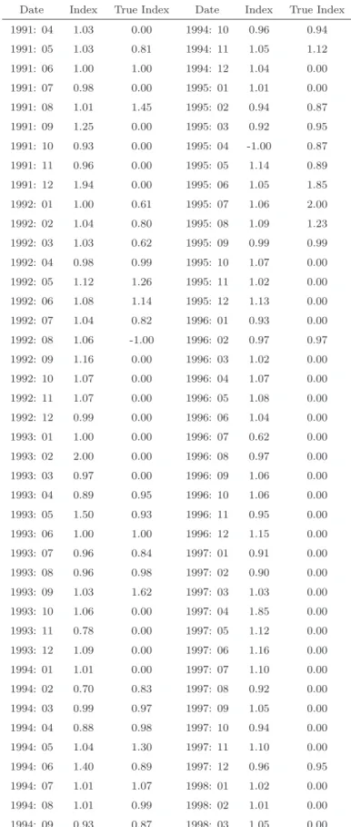
Table 3: Weymark Index and “True” Weymark Index: 1991: 04 - 1998: 03

Date Index True Index Date Index True Index 1991: 04 1.03 0.00 1994: 10 0.96 0.94 1991: 05 1.03 0.81 1994: 11 1.05 1.12 1991: 06 1.00 1.00 1994: 12 1.04 0.00 1991: 07 0.98 0.00 1995: 01 1.01 0.00 1991: 08 1.01 1.45 1995: 02 0.94 0.87 1991: 09 1.25 0.00 1995: 03 0.92 0.95 1991: 10 0.93 0.00 1995: 04 -1.00 0.87 1991: 11 0.96 0.00 1995: 05 1.14 0.89 1991: 12 1.94 0.00 1995: 06 1.05 1.85 1992: 01 1.00 0.61 1995: 07 1.06 2.00 1992: 02 1.04 0.80 1995: 08 1.09 1.23 1992: 03 1.03 0.62 1995: 09 0.99 0.99 1992: 04 0.98 0.99 1995: 10 1.07 0.00 1992: 05 1.12 1.26 1995: 11 1.02 0.00 1992: 06 1.08 1.14 1995: 12 1.13 0.00 1992: 07 1.04 0.82 1996: 01 0.93 0.00 1992: 08 1.06 -1.00 1996: 02 0.97 0.97 1992: 09 1.16 0.00 1996: 03 1.02 0.00 1992: 10 1.07 0.00 1996: 04 1.07 0.00 1992: 11 1.07 0.00 1996: 05 1.08 0.00 1992: 12 0.99 0.00 1996: 06 1.04 0.00 1993: 01 1.00 0.00 1996: 07 0.62 0.00 1993: 02 2.00 0.00 1996: 08 0.97 0.00 1993: 03 0.97 0.00 1996: 09 1.06 0.00 1993: 04 0.89 0.95 1996: 10 1.06 0.00 1993: 05 1.50 0.93 1996: 11 0.95 0.00 1993: 06 1.00 1.00 1996: 12 1.15 0.00 1993: 07 0.96 0.84 1997: 01 0.91 0.00 1993: 08 0.96 0.98 1997: 02 0.90 0.00 1993: 09 1.03 1.62 1997: 03 1.03 0.00 1993: 10 1.06 0.00 1997: 04 1.85 0.00 1993: 11 0.78 0.00 1997: 05 1.12 0.00 1993: 12 1.09 0.00 1997: 06 1.16 0.00 1994: 01 1.01 0.00 1997: 07 1.10 0.00 1994: 02 0.70 0.83 1997: 08 0.92 0.00 1994: 03 0.99 0.97 1997: 09 1.05 0.00 1994: 04 0.88 0.98 1997: 10 0.94 0.00 1994: 05 1.04 1.30 1997: 11 1.10 0.00 1994: 06 1.40 0.89 1997: 12 0.96 0.95 1994: 07 1.01 1.07 1998: 01 1.02 0.00 1994: 08 1.01 0.99 1998: 02 1.01 0.00 1994: 09 0.93 0.87 1998: 03 1.05 0.00

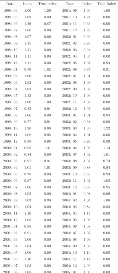
Table 4: Weymark Index and “True” Weymark Index: 1998: 04 - 2005: 01

Date Index True Index Date Index True Index 1998: 04 1.00 1.00 2001: 09 1.00 1.00 1998: 05 1.09 0.00 2001: 10 1.24 0.00 1998: 06 1.16 0.87 2001: 11 0.63 0.00 1998: 07 1.06 0.00 2001: 12 1.20 0.00 1998: 08 1.07 0.00 2002: 01 0.99 0.00 1998: 09 1.15 0.00 2002: 02 0.98 0.00 1998: 10 1.11 0.00 2002: 03 0.94 0.00 1998: 11 1.11 0.00 2002: 04 1.05 0.00 1998: 12 1.11 0.00 2002: 05 1.07 0.94 1999: 01 0.99 1.02 2002: 06 0.95 0.91 1999: 02 1.06 0.00 2002: 07 1.01 0.00 1999: 03 1.02 0.00 2002: 08 1.09 0.00 1999: 04 1.03 0.00 2002: 09 1.07 0.00 1999: 05 1.13 0.00 2002: 10 1.06 0.00 1999: 06 1.00 1.00 2002: 11 1.02 0.00 1999: 07 0.82 0.91 2002: 12 1.05 0.00 1999: 08 1.06 0.00 2003: 01 1.01 0.94 1999: 09 0.77 0.91 2003: 02 0.38 0.95 1999: 10 1.20 0.00 2003: 03 1.03 1.22 1999: 11 1.08 0.95 2003: 04 1.01 0.00 1999: 12 0.99 0.98 2003: 05 0.96 0.99 2000: 01 0.95 1.31 2003: 06 1.06 1.13 2000: 02 0.84 0.00 2003: 07 1.02 1.01 2000: 03 0.97 0.91 2003: 08 1.07 0.73 2000: 04 1.01 1.01 2003: 09 0.88 0.94 2000: 05 0.98 0.00 2003: 10 0.88 0.93 2000: 06 0.97 0.00 2003: 11 1.02 1.03 2000: 07 1.06 0.00 2003: 12 0.88 0.95 2000: 08 1.05 0.00 2004: 01 0.98 0.99 2000: 09 1.03 0.00 2004: 02 1.04 1.06 2000: 10 1.04 0.00 2004: 03 0.84 0.93 2000: 11 1.10 0.00 2004: 04 1.14 0.00 2000: 12 1.08 0.00 2004: 05 1.08 0.00 2001: 01 0.98 0.00 2004: 06 1.08 0.00 2001: 02 0.91 0.00 2004: 07 1.07 0.00 2001: 03 1.06 0.00 2004: 08 1.09 0.00 2001: 04 1.04 0.00 2004: 09 1.08 0.00 2001: 05 1.06 0.00 2004: 10 1.13 0.00 2001: 06 1.10 0.00 2004: 11 1.14 0.00 2001: 07 1.03 0.00 2004: 12 2.00 0.00 2001: 08 1.08 0.00 2005: 01 1.00 0.00

Table 5: Distribution of the Weymark Index and the True Weymark Index Range Percentage of WI Percentage of TWI

ω ≥ 1 66.87% 12.65% 1 > ω ≥ 0.9 23.49% 17.47% 0.9 > ω ≥ 0.7 6.63% 7.23% 0.7 > ω ≥ 0.5 1.81% 1.20% 0.5 > ω ≥ 0.0 0.60% 60.84% ω < 0 0.60% 0.60%

Table 6: Regression Results

Variable Estimate Std Error Constant 1.063*** 0.020 True Weymark Index -0.087** 0.328

Appendix

According to Weymark (1997), the structure of the representative small-open economy is described, in logarithms, as follows:

yt− ¯y = α[pt− E(pt|Ωt−1)] + νty, (4) pt = apNt + (1 − a)p T t, (5) pT t = p∗t + et (6) it= i∗t + E(et+1|Ωt) − et, (7) md t − pt= b1yt− b2it+ νtm, (8) mst = m s t−1+ ∆dt+ ∆rt, (9) ∆rt= −¯ρt∆et, (10)

where yt is real domestic output with potential level of output, ¯y. pt is the domestic price

level while pT

t and pNt are prices for traded and non-traded goods, respectively. it is the

domestic interest rate level. et is the exchange rate expressed in terms of the domestic

currency cost of one unit of foreign currency. md

t and mst are money demand and supply,

respectively. ∆dtand ∆rtdenote change in domestic credit and foreign exchange reserves,

where both dtand rtare expressed as a proportion of the money base. νty and νtmrepresent

stochastic disturbances of output and money demand, respectively. Finally, Ωt denotes

the information set at time t. All variables with asterisks are the foreign counterparts of the relevant domestic variables.

Equation (4) represents equilibrium condition for goods market. Equation (5) defines the domestic price index. Equation (6) is the purchasing power parity, and equation (7) is the uncovered interest rate parity. Equation (8) denotes real domestic money demand function while equation (9) describes the supply of money as depending on the inherited money base, ms

t−1, the change in domestic credit, ∆dt, and the change in foreign

exchange reserves, ∆rt. Finally, equation (10) indicates how central bank change the

foreign exchange reserves in response to contemporaneous changes in the exchange rate. As mentioned in Section 2, the Weymark index is calculated as follows:

ωt=

∆rt

(1/η)∆et+ ∆rt

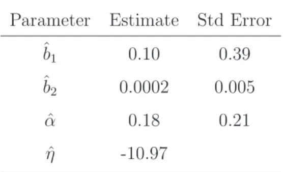
Table 7: Estimation Results Parameter Estimate Std Error

ˆb1 0.10 0.39 ˆb2 0.0002 0.005 ˆ α 0.18 0.21 ˆ η -10.97

where η = −[b2 + (1 − a)(1 + αb1)]−1. Thus we need to estimate b1, b2 and α in order

to construct ωt. Following Weymark (1997), the parameter, a, is simply computed as the

average ratio of the value of imports to GDP.

We obtain model-consistent estimates of b1, b2 and α from equations (4) and (8),

where E(pt|Ωt−1) is estimated by E(pt|Ωt) = δ0 +

P3

j=1δ1jpt−j. The potential output ¯y

is derived using the Hodrick-Prescott (HP) filter.7 _{For data found to be I(1), estimation}

is undertaken using first-difference. The estimation results are reported in Table 7. All of the parameters are correctly signed but statistically insignificant. This may due to the small sample span we examine.

7

Rather than using HP filter to derive ¯y, we have also followed Weymark (1997) to estimate η by 2SLS and obtained ˆη= −13.59.

References

Bofinger, P., and T. Wollmershauser (2003): “Managed Floating as a Monetary Policy Strategy,” Economics of Planning, 36(2), 81–109.

Calvo, G. A., and C. M. Reinhart (2002): “Fear of Floating,” Quarterly Journal of Economics, 117(2), 379–408.

Fischer, S. (2001): “Exchange Rate Regimes: Is the Bipolar View Correct?,” Finance and Development, 38(2), 18–21.

Frankel, J. A., andS. Wei(1994): “Yen Bloc or Dollar Bloc? Exchange Rate Policies in the East Asian Economies,” in Macroeconomic Linkage: Saving, Exchange Rates, and Capital Flows, ed. by T. Ito, and A. Krueger. NBER and University of Chicago Press.

Jeisman, S. (2005): “Exchange Market Pressure in Australia,” Quarterly Journal of Business and Economics, 44(1-2), 13–27.

Kohlscheen, E.-W. (2000): “Estimating Exchange Market Pressure and Intervention Activity,” Banco Central do Brasil, Working Paper Series n.9.

McKinnon, R. I.(2001): “After the Crisis, the East Asian Dollar Standard Resurrected: An Interpretation of High-Frequency Exchange-Rate Pegging,” in Rethinking the East Asian Miracle, ed. by J. Stiglitz, and S. Yusuf. World Bank and Oxford University Press.

Sarno, L., and M. P. Taylor (2002): The Economics of Exchange Rates. Cambridge, 1st edn.

Weymark, D. N. (1997): “Measuring the Degree of Exchange Market Intervention in a Small Open Economy,” Journal of International Money and Finance, 16(1), 55–79.