Sensorless Speed Tracking of Induction
Motor With Unknown Torque Based
on Maximum Power Transfer
Hou-Tsan Lee, Member, IEEE, Li-Chen Fu, Senior Member, IEEE, and Hsin-Sain Huang
Abstract—In this paper, we first derive the maximum power
transfer theorem for an induction motor. Then, a nonlinear indi-rect adaptive sensorless speed tracking controller for the motor with the maximum power transfer is proposed. In this controller, only the stator currents are assumed to be measurable. The rotor flux and speed observers are designed to relax the need of flux and speed measurement. In addition, the rotor resistance estimator is also designed to cope with the problem of the fluctuation of rotor resistance with temperature. Stability analysis based on Lyapunov theory is also performed to guarantee that the controller design here is stable. Finally, the computer simulations and experiments are conducted to demonstrate the satisfactory tracking perfor-mance of our design subject to maximum power transfer.
Index Terms—Adaptive control, induction machine, maximum
power transfer, sensorless.
NOMENCLATURE Number of pole pairs. Slip angular velocity. Stator self-inductance. Rotor self-inductance. Mutual inductance. Stator resistance. Rotor resistance.
Stator currents in – frame (reference fixed frame).
Rotor fluxes in – frame (reference fixed frame).
Stator voltages in – frame (reference fixed frame). Electric torque. Load torque. Torque constant. Rotor inertia. Damping coefficient.
Manuscript received January 10, 2001; revised December 17, 2001. Abstract published on the Internet May 16, 2002. This work was supported by the Na-tional Science Council, R.O.C., under Grant NSC 90-2213-E-002-054.
H.-T. Lee was with the Department of Electrical Engineering, National Taiwan University, 106 Taipei, Taiwan, R.O.C. He is now with ChungHwa Telecom Company, Keelung, Taiwan, R.O.C. (e-mail: houtsan@ieee.org; houtsan@cht.com.tw).
L.-C. Fu is with the Department of Electrical Engineering and Department of Computer Science and Information Engineering, National Taiwan University, 106 Taipei, Taiwan, R.O.C. (e-mail: lichen@ccms.ntu.edu.tw).
H.-S. Huang was with the Department of Electrical Engineering, National Taiwan University, 106 Taipei, Taiwan, R.O.C. He is now with Quanta Display Inc., Taipei, Taiwan, R.O.C. (e-mail: hhs789@tpts6.seed.net.tw).
Publisher Item Identifier 10.1109/TIE.2002.801245.
Stator voltage vector. Rotor voltage vector. Stator flux vector. Rotor flux vector. Stator power. Effective power. . . . . . . . . . . I. INTRODUCTION
I
N THE EARLY research on induction motors, all system states are assumed to be measurable and all parameters are considered known. Under these assumptions, techniques such as field orientation [1] and input–output feedback linearization [2], [3] are utilized to design the controller. In particular, the controller in [3] is adaptive with respect to both load torque and rotor resistance variations. In these schemes the flux sensors are required, which makes them impractical for implementation. Therefore, the flux observers are then designed to relax the need of flux measurement [4], [5]. These flux observers are designed under the assumption that the rotor resistance is known. Gener-ally, the value of rotor resistance may drift due to heating of rotor and the observers proposed above are sensitive to such value. Therefore, efforts have been made to design an estimator of the rotor resistance [6], [7]. Following this research, more efforts have been made to design controllers and flux observers which are adaptive with respect to both system parameters and/or load torque [8]–[11].There are many works concerning the sensorless control problem, in which the vector control technique is utilized, and the research results on sensorless vector control have been proposed [12], [13], of which analyses are mainly based on the steady-state behavior and only rough proofs are supplied. In [14], the speed observer is designed and analyzed based on the Lyapunov stability theory. Both observer and controller apply the direct adaptive control scheme coping with the unknown rotor resistance. Because of the complex dynamics of the 0278-0046/02$17.00 © 2002 IEEE
induction motor, the overall system analysis is also complex. In [15], an indirect adaptive scheme is proposed. The controller design is under the assumption that all states are measurable and all parameters except the load torque are known a priori. However, the controller is not actually realizable because the rotor resistance and speed are not available. Therefore, the observers and estimators are designed to provide estimates of those states and parameters, which then replace those measur-able quantities so that the closed-loop controller is realizmeasur-able and stable. Here, we follow this trend to design a full nonlinear adaptive sensorless controller to achieve both speed tracking and maximum power transfer based on the setup with speed and flux observer.
Given the above observation, the developed adaptive con-troller achieves both objectives of speed tracking and maximum power transfer despite lack of precise information of rotor re-sistance, payload, and speed. Specifically, to relax the need of speed and flux measurement, we design a set of adaptive rotor speed and flux observer and a rotor resistance estimator in order to replace those unavailable signals in controller design. In this paper, the simulation and experimental results are also given to verify the performance of the controller design.
This paper is organized as follows. In Section I, motivation of this research, related research results in the literature, and the research contribution are addressed. The main part of this paper is from Section II to Section IV. The maximum power transfer theory is derived in Section II and will be used in controller de-sign in Section IV. Section III includes the procedure of observer design which is then analyzed in detail. Also, the simulation and experimental results are provided in Section V and Section VI, respectively. Finally, we make some conclusions in Section VII.
II. MAXIMUMPOWERTRANSFER OFINDUCTIONMOTOR If we define a new – frame, called the – frame, rotating in speed to make the stator current vector lie on the axis, a new set of governing dynamic equations can be derived. We rearrange these equations in vector form as
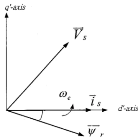
(2.1) where the symbols are defined in the Nomenclature. The spatial diagram of vectors in the reference frame is shown in Fig. 1. The relationship between the flux and the currents are as follows:
so that
where (2.2)
Fig. 1. Spatial vector diagram of induction motor ind –q reference frame. Taking the relationship (2.2) into (2.1), we have the new dy-namic equation
(2.3) Since the stator current exists only along the axis, is, in fact, equal to a scalar . After substituting for the vector and the scalar in (2.3), we can then derive the following equation after splitting the real part and the imaginary part of the original equation:
(2.4)
Rearranging (2.4) with and ,
we come up with the new set of equations as follows:
(2.5)
For simplicity, we define and it
has been verified that in [16].
In the steady state, the stator current is defined as , where is the equivalent impedance at the stator input. Thus, the input power of the induction motor can be defined as
which is related to in the steady state. Referring to (2.3) and (2.4), the input power can be briefly noted as
Note that only the terms with rotor flux are transferred to the rotor part of the induction motor and the rest of them become
the loss. Thus, the power transferred to the rotor of induction motor can be rearranged by applying (2.4) and (2.5) as
Now, all the terms in the imaginary parts are obviously summed up to zero, and the terms with are the power transferred into the rotor. Therefore, those terms with can be expressed as
On the other hand, the matrix product
can also be expanded into the following equation:
by applying (2.4), (2.5), and the definition of . Therefore, the power transferred to the rotor of induction motor in the steady
state is maximal if and only if
be-comes maximal. Under the constraint that is a fixed constant at any time, where (or ) is the - (or -) axis rotor flux, the latter objective can obviously be achieved by real-ization of the field-oriented control law in the following (using the optimal LaGrange method with a bounded condition [20]):
(2.6)
which clearly satisfies the voltage constraint “ ” at any time.
In the above discussion, we have made the conclusion that the maximum power transfer can be achieved when (2.6) is satisfied. It implies that the stator voltage vector and the rotor flux vector are perpendicular to each other and such relation-ship holds in the fixed reference frame. Therefore, we can also derive the maximum power transfer property here in the fixed reference frame under the constraints
(2.7)
III. OBSERVERDESIGN
In general, the dynamics of an induction motor can be ex-pressed as [18]
(3.1)
where the meanings of all the variables are listed in the Nomen-clature. As mentioned in Section I, the control objective is to fulfill the requirement of speed tracking but under the adverse conditions that no speed and flux measurements are allowed and the rotor resistance is unknown a priori. Furthermore, the whole developed scheme will satisfy the so-called maximal power transfer property. Given such circumstances, the speed tracking controller will have to be developed with ingenious design of various observers which meet the needs of estimating unknown parameters as well as unmeasurable states.
Before we proceed to derive the observers and the controller in the following section, some assumptions will be introduced below to manifest the problem and to make it more tractable.
Assumptions:
(A1) All parameters of the induction motor are known, ex-cept the rotor resistance .
(A2) Among all states, only the stator currents are measur-able.
(A3) The desired rotor speed should be a bounded smooth function with known first- and second-order time derivatives.
(A4) The load torque is an unknown constant.
Assumption (A1) comes from the uncertainty of rotor resis-tance. Its value may vary up to 150% during the operation due to variation of temperature or working condition. Assumption (A2) is a realistic consideration in the actual application of in-duction motors as has been mentioned in Section I. Finally, as-sumptions (A3) and (A4) are mainly for technical soundness and are also quite realistic in practical applications. Later in our ex-periment, step-type desired speed trajectory in fact can be shown to be permissive to our scheme, i.e., assumption (A3) can, in re-ality, be relaxed.
As has been mentioned earlier, the rotor resistance is as-sumed unknown due to its fluctuation with temperature and the rotor speed is not measurable since no speed sensor is mounted. To cope with this, we first rewrite and as
where is the nominal value of rotor resistance and is the desired rotor speed. Apparently, and stand for the dis-crepancies from what we know about and . For subsequent simplicity of the problem, we will assume is a constant and
, although it is not a constant, will be slowly varying, i.e., is small enough. According to the structure of the dynamics in (3.1), the observers are proposed as follows:
(3.2)
where , and and are
the auxiliary control signals to be designed later. Note that the symbol above indicates an observed value whereas the symbol
denotes the associated observation error. Now, we can derive the error dynamics by subtracting (3.2) from (3.1) to yield
(3.3) By careful observation, the right-hand side (RHS) of the first two equations in (3.3) has many terms identical to those on the RHS of the last two equations also in (3.3), but they are with different signs. In order to utilize this property to cancel the un-measurable terms, we introduce two auxiliary observation errors as
(3.4)
To force ( ) to approach zero asymptotically, we
introduce another set of auxiliary signals ( ) and ( ) into the system, which are related as
(3.5) Note that the control signals ( ) are devised to cancel the coupled terms as
(3.6)
Obviously, and are design variables, but and then
will not be available from (3.5). After substituting them into the first two equations of (3.3) and defining new symbols
then, we get
(3.7)
where and .
After investigating the error dynamics of the stator current observer, we now turn to the study of the flux observer. The flux observer dynamics will not be analyzed directly, but instead will be through the analysis of ( ). Our intention is to define control signals ( ) as follows:
(3.8) so that
(3.9) So far, we have derived the error dynamics of the observation errors of the stator currents, rotor flux, and those of the auxiliary signals and have specified the controller input ( ). However, the variables ( ) and ( ) are not yet defined, but will be specified in the later Lyapunov stability analysis so that stability condition will hold in both observer and estimator design.
Consider the following Lyapunov function candidate:
(3.10) where the control gains , and are all strictly positive. By carefully evaluating the time derivative of and the means
of definitions of , can be made more concise as
follows:
Here, we introduced four additional functions which
are similar to in order to simplify the above
ex-pression of , where the difference between and
lies in that ( ) are replaced by ( ) since and are not obtainable as has been mentioned earlier. Thus, considerable simplification of will be contributed by the fol-lowing assignment:
(3.11)
so that readily becomes
(3.13)
where and . We now adopt
variable-structure design (VSD) in our observer design in order to assure the upper bound of the RHS in (3.13) to be a definite negative sign. To proceed, we first obtain the upper bound of ( ) in the following lemma.
Lemma 3.1: The upper bound of ( ) can be explicitly derived by proper design of ( ) as some positive constants
and .
Proof: The proof of the lemma can be referred to in [15]. Q.E.D.
Since the upper bound ( ) is acquired from Lemma 3.1, we can design the additional functions ,
, and and devise
the control signals as follows:
where
if if
Seemingly, and may not be realizable due to lack of knowl-edge of and . However, in reality, one can always choose higher gains , , initially to establish close observa-tions first, i.e., and tend to small residual values and then gradually reduce the gains. As the result of the above designs,
becomes
(3.14) From (3.10) and (3.14), it immediately follows
is bounded and (3.15)
In order to confirm the above claim on the proper design of and , we soon show that and will converge to zero under appropriate conditions besides the high gain condition in the following. Before that, we first present the following working lemmas.
Lemma 3.2: The states ( ) are bounded provided ( ) are bounded in finite time.
Proof: The proof of the lemma can be referred to in [15]. Q.E.D.
Now, we need to establish another result, which guarantees
boundedness of presuming boundedness of ( ) in
Lemma 3.3 as follows.
Lemma 3.3: The rotor speed is bounded if ( ) is bounded.
Proof: The proof of the lemma can be referred to in [15]. Q.E.D.
Since is bounded from the previous argument, it follows that is also bounded. That will lead to the following Lemma 3.4 to guarantee the boundedness of the estimated rotor flux.
Lemma 3.4: The error dynamics of the rotor flux in (3.2) are rearranged in vector form as
(3.16) Thus, if the estimate of the rotor resistance, , is kept posi-tive and bounded away from the origin, then ( ) will be bounded provided ( ) are bounded.
Proof: The proof of the lemma can be referred to in [15]. Q.E.D.
From Lemma 3.4, ( ) are bounded, which together
with the boundedness of and from (3.15) readily implies that ( ) are also bounded from (3.4). Then, it follows from (2.5) that ( ) are thus bounded. Now, from (3.3) are proved bounded as well since signals on the RHS are all bounded, which together with the property that is revealed in (3.15) implies
and
via Barbalat’s Lemma [19]. Now, we have proved the conver-gence of the observation errors of the stator currents under the premises of Lemma 3.4. The next problem is to prove if the es-timation errors of the rotor resistance and the rotor speed have the same convergence property.
To solve this problem, we first make the following definitions:
and rearrange the error dynamics in (3.7) and those equations in (3.11) to yield
(3.17) where
Now, to prove tends to zero asymptotically, we have to use the conclusion stated in Lemma 3.5 given below.
Lemma 3.5: The system with the form
(3.18)
is exponentially stable if and only if is persistently exciting (PE), i.e., there exist two positive constant and such that
Proof: The proof of the lemma can be referred to in [15]. Q.E.D.
By Lemma 3.5, we conclude that the system (3.18) is expo-nentially stable provided is PE. However, from (3.17) the asymptotic convergence property of and may no longer hold due to the forcing term added to the homogeneous system (3.18). To cope with this, we first note that the forcing term in (3.17) with respect to the homogeneous part in (3.18) will be ultimately in the order of the magnitude of under the premises of Lemma 3.4, since ( ) will then tend to zero. Thus, in our observer design, we gradually decrease the values of the control signals ( ) to zero as tends to zero. Under such design, the equilibrium point ( ) of (3.17) re-mains asymptotically stable so that ( ) tends to zero asymptotically. In turn, this will confirm the hypothesis where the rotor resistance estimate is kept positive and bounded away from the origin in Lemma 3.4. Finally, from (3.3) the fact that and tend to zero asymptotically and that the control signals and converge to zero by (3.8), and will also tend to zero asymptotically. Up to now, we can conclude the satisfactory convergence property provided PE condition holds and ( ) are bounded. After the analysis above, the design of observers can be detailed as in Theorem 1 shown below, whose proof is self-evident from the above arguments.
Theorem 1: Consider the induction motor whose dynamics are governed by (3.1) under the assumptions (A1)–(A4). If the stator current observers and the rotor flux observers are de-signed as in (3.2), where
then the observed speed and flux of the rotor will be driven to the actual speed and flux and the estimate of rotor resistance will also converge to the actual one subject to the control signals designed as follows:
where the auxiliary signals are designed as follows:
for some constants .
IV. CONTROLLERDESIGN
In this section, the controller that achieves speed tracking with maximal power transfer is proposed. The controller can also overcome the variation of the unknown load torque under the indirect adaptive control scheme, i.e., the observer provides all the necessary information to the controller, such as unknown parameter and unmeasurable states. Therefore, throughout the rest of sections we will proceed with our discussion pretending all parameters are known and all state signals are measurable. Thus, all notations used in the sequel will be without “” attached. Before we apply the input-output linearization scheme, we will introduce an assumption on model so that such a scheme can hereby actually applicable. Recall the mathematical model of the induction motor is derived in Section III and is rewritten here in (4.1), where all notations introduced are explained in the Nomenclature.
Assumption (A5): The damping term of the mechanical sub-system will have negligible effect relative to our control objec-tive so that it will be omitted from our controller design. The new system dynamics of the induction motor are as follows:
(4.1)
where the symbols are defined in the Nomenclature. First, we define the load torque variation as
where is the nominal value of the load torque and is the actual value. Now, we introduce a set of coordinates as follows:
Rewrite the dynamical (4.1) in terms of the new coordinate variables with the maximal power transfer property (see [21]) as
(4.2) where
To make the representation more concise, we introduce another coordinate transformation
(4.3)
where is the estimate of the load torque variation . Define the estimation error of the load torque variation as follows:
(4.4) Substituting the new coordinates in (4.3) and the new definition in (4.4) into the system dynamics (4.2), we then obtain the fol-lowing set of differential equations as:
(4.5) Now we introduce some modification into the decoupling con-trol in (2.7) as shown below
TABLE I
SPECIFICATIONS ANDPARAMETERS OF THECONTROLLEDMOTOR
and , where .
Up to this point, the adaptive term has not yet been determined, but it will be defined later. Note that the decoupled dynamics can be expressed concisely as
(4.6) To claim our control objective, it is natural to build a reference model a priori and generate the relevant reference signal. The reference model can be defined as follows:
(4.7)
where
Before we start to design and analyze the controller, Lemma 4.1 is given to ensure the feasibility of the controller.
Lemma 4.1: The stator currents ( , ) will be bounded pro-vided the input power is bounded in a realistic operating en-vironment, i.e., the stator voltages are kept bounded.
Proof: The proof of the lemma can be referred to in [21]. Q.E.D.
Theorem 2: If the dynamic system of an induction motor can be described as in (4.5), then the rotor speed can be driven to the desired speed with unknown load torque by the controller designed as (2.7), where
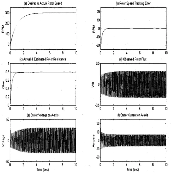
Fig. 2. Simulation result of! = 300(1 0 e ) r/min with unknown R and T . subject to the payload adaptation law as
Proof: To analyze the convergence property of the previ-ously developed controller, we first define the error signals
For convenience of analysis, we rearrange the error dynamics as
(4.8)
where
Now, letting block diag , the positive-definite
symmetric solution to the Lyapunov equation
where block diag and , are
positive-defi-nite symmetric matrices.
To proceed with the Lyapunov analysis, we define a Lya-punov function candidate as
whose time derivative can be then derived as
(4.9)
If we let , then from (4.4), it
immedi-ately follows that
which reveals our adaptation law of the load torque. It is de-signed to overcome variation of load torque, which then helps to simplify the RHS of (4.9) to yield
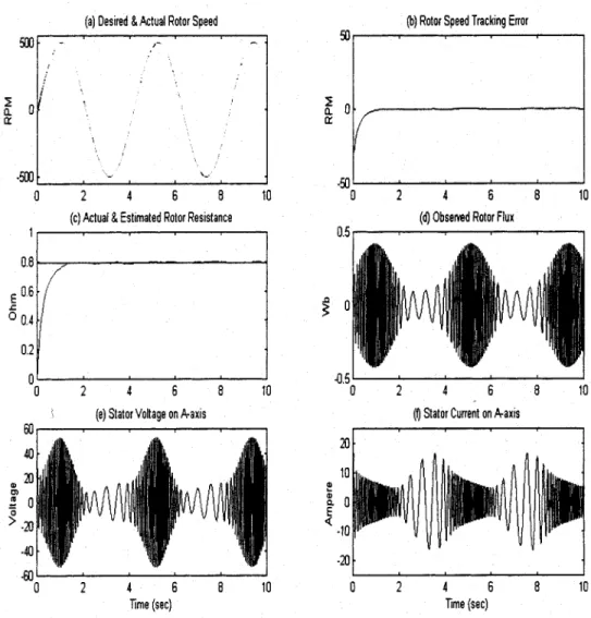
Fig. 3. Simulation result of! = 500 sin(1:5t) r/min with unknown R and T . The fact that is negative implies that , are bounded and the negative quadratic form of the RHS of (4.10) implies that
.
Since is bounded, from (4.6) it can be proved that the states ( , ) are bounded, which immediately implies that is bounded. In addition, according to the fact that both and
are bounded from (4.4), the boundedness of can also be proved. Then, from (4.3) we know that
is bounded and it immedi-ately follows that ( ) is bounded. Due to the fact that , then it can be directly shown that is bounded. If we recall the power formula
which immediately deduces that is also bounded.
With the results from Lemma 4.1 and from the definition of , we can also prove that is a bounded function. Then, from (4.6) and the fact that is a bounded function, it fol-lows that
are bounded (4.11)
TABLE II
VARIOUSGAINS ANDINITIALVALUES FORSPEEDCONTROL INCASE1
Considering (4.8), we can prove that is bounded. There-fore, from Barbalat’s Lemma, we have the final result:
. In other words, the controller goal
Q.E.D. Up to this point, we thus conclude that through the adap-tive input-output feedback linearization, a speed controller with
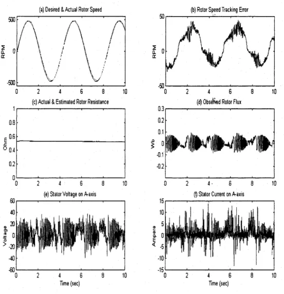
Fig. 4. Simulation result of speed tracking benchmark result.
TABLE III
VARIOUSGAINS ANDINITIALVALUES FORSPEEDCONTROL IN
BENCHMARKTEST
maximum power transfer property is designed as in Theorem 2 and it can be further proved the controller can operate in the en-vironment whose load torque is an unknown constant.
V. SIMULATIONRESULTS
The simulation and experiment are done with a four-pole three-phase squrrel-cage induction motor with rated power 3 hp with a 1000-pulse/rev encoder which is manufactured by TACO
Fig. 5. Block diagram of experiment system.
Fig. 7. Experimental result of! = 300(1 0 e ) r/min with no load. Company Ltd., Taiwan, R.O.C., with a delta-connected stator. Detailed parameters and specifications will be found Table I. The software we adopt in simulation is Simulink 3.0 and Matlab 5.2, an excellent product of The MathWorks Inc., Natick, MA. In addition, we use Simu-Drive to combine the motor control card with the Simulink/Real Time Workshop. Then, we can di-rectly apply the simulation program to proceed with our exper-iment.
In the speed tracking problem, we design the desired speed as a smooth function which satisfies our assumption (A3). Then, the desired speed is a smooth function with known first- and second-order time derivatives. The simulation results will show the performance of the proposed control scheme. In addition, we will show the properties of the state observers and the parameter estimator.
Case 1—Speed Tracking With Unknown Rotor Resistance and Load Torque: We design two kinds of speed trajectories and the results are shown in Figs. 2 and 3. About the variation of the rotor resistance, its nominal value is 0.53 and it is assumed to vary 50% due to the temperature excursion, i.e., it can reach the maximum value 0.795 . Furthermore, the load torque is assumed to be 5.0 N m. There are several parts in each figure. The results of speed tracking are shown in Fig. 2(a) and (b) and Fig. 3(a) and (b). Figs. 2(c) and 3(c) show the tracking of rotor
resistance, and Figs. 2(d) and 3(d) are the observed rotor flux on the axis in the stationary reference frame. Fig. 2(e) and (f) and Fig. 3(e) and (f) are stator voltage and current on the axis in the stationary reference frame, respectively. Finally, the controller gains and observers gains are shown in Table II.
From these figures, we can find that the tracking error will tend to zero asymptotically when time goes to infinity. Further-more, the stator current response, stator voltage, and the per-formance of flux tracking are satisfactorily shown. From the results, we can conclude that our controller can overcome the uncertainty of rotor resistance and load torque.
Case 2—Speed Tracking Benchmark Results: We perform computer simulations for the benchmark example [17]. The rotor speed is required to change between these values: ,
0.1 , 0.25 , and 1.5 during the time interval
[0,10] s, where the is 500 r/min. The load torque is
0.5 at s and changes to 0.25 at s,
where the is 10 N m, and the rotor resistance variation is 30%.
The simulation result for the speed tracking benchmark is shown in Fig. 4. In order to apply the theory developed in this paper, especially the assumption on the smoothness of desired speeds, we adopt a smooth function to approximate the step function so that the desired speed is continuously differentiable.
Fig. 8. Experimental result of! = 500 sin(1:5t) r/min with no load. One can find that the speed tracking is insensitive to the load torque variation. Furthermore, the speed tracking error will con-verge despite the variation of the desired rotor resistance. How-ever, when the rotor resistance variation is considered, the error convergence for speed tracking will be slightly slower. Finally, the various gains and initial values used for simulation are listed in Table III.
VI. EXPERIMENTALRESULTS
In this section, we first show the overall system in Figs. 5 and 6. Then, in order to check the performance, we have done two experiments with exponential and sinusoidal speed command as in Figs. 7 and 8. For all of the cases, they are subjected to the load free condition. And the nominal rotor resistance is set as 0.53 (different to the maximal 0.795 in simulation).
To make the experiment the realization of the simulation, the desired speed trajectories of the experiments are assigned as the same as those in simulation. Therefore, it is easy to validate the tracking performance of the proposed controller, and we con-duct an experiment to compare our results with those from an-other controller based on the same scheme of I/O linearization [3], [21]. Fig. 9 shows the performances of both control schemes
under the same conditions (with speed feedback) with the speed command of 120 rad/s.
The control performance can be summarized as follows. • Due to the effect of load torque and damping effect, the
rotor hardly rotates very smoothly, especially in the case of extremely low speed. Therefore, there will be a rel-atively large error when the rotor is operated near the zero-crossing point.
• For the exponential trajectories, the speed error is nearly limited within 10 r/min. In addition, the speed error is larger for the sinusoidal trajectories because of the phase shift, but are always limited within 50 r/min.
• The estimated rotor resistance will approach the actual value.
• Both the stator current and the rotor speed error are smaller than the compared control scheme [3].
VII. CONCLUSION
In this paper, we have proposed an indirect adaptive sensor-less controller with maximum power transfer based on the I/O feedback linearization scheme. In Section II, we derived the maximum power transfer theory via the concept of coupled field and Lagrange multiplier. We can achieve not only better energy
Fig. 9. Comparison of proposed control scheme and [3] at speed 120 rad/s (see [21]).
efficiency through this theory, but can also add one constraint to our control signals [21]. To solve the speed tracking problem, we use the I/O feedback linearization scheme to design our con-troller. In addition, to cope with the situation where some states, such as flux and rotor speed, are not available and the param-eter (rotor resistance) has a shift problem, we first construct the state observers and the rotor resistance estimator to provide the asymptotic accurate values of the states and the parameter. Then, we proposed an adaptive I/O feedback linearization con-troller subject to the unknown load torque. Finally, we substi-tute the observed states and estimated rotor resistance into the controller for realization. Finally, both the simulation and ex-perimental results confirm the effect of our control design and the power-saving effect.
REFERENCES
[1] W. Leonhard, “Microcomputer control of high dynamic performance AC-drives—A survey,” Automatica, vol. 22, pp. 1–19, 1986.
[2] A. D. Luca and G. Ulivi, “Design of an exact nonlinear controller for in-duction motors,” IEEE Trans. Automat. Contr., vol. 34, pp. 1303–1307, Dec. 1989.
[3] R. Marino, S. Peresada, and P. Valigi, “Adaptive input-output linearizing control of induction motors,” IEEE Trans. Automat. Contr., vol. 38, pp. 208–221, Feb. 1992.
[4] A. Bellini, G. Figalli, and G. Ulivi, “Adaptive and design of a micro-computer-based observer for an induction machine,” Automatica, vol. 24, pp. 549–555, 1988.
[5] G. C. Verghese and S. R. Sanders, “Observers for flux estimator in in-duction mahines,” IEEE Trans. Ind. Electron., vol. 35, pp. 85–94, Feb. 1988.
[6] J. Stephan, M. Bodson, and J. Chiasson, “Real-Time estimation of the parameters and fluxes of induction motors,” IEEE Trans. Ind. Applicat., vol. 30, pp. 746–748, May/June 1993.
[7] R. Marino, S. Peresada, and P. Tomei, “Exponentially convergent rotor resistance estimation for induction motors,” IEEE Trans. Ind. Electron., vol. 42, pp. 508–515, Oct. 1996.
[8] J. Hu and D. M. Dawson, “Adaptive control of induction motor systems despite rotor resistance uncertainty,” in Proc. American Control Conf., June 1996, pp. 1397–1402.
[9] J. H. Yang, W. H. Yu, and L. C. Fu, “Nonlinear observer-based adaptive tracking control for induction motors with unknown load,” IEEE Trans.
Ind. Electron., vol. 42, pp. 579–586, Dec. 1995.
[10] R. Marino, S. Peresada, and P. Tomei, “Adaptive observer-based control of induction motors with unknown rotor resistance,” Int. J. Adapt.
Con-trol Signal Process., vol. 10, pp. 345–362, 1996.
[11] , “Global adaptive output feedback control of induction motors with unknown rotor resistance,” in Proc. 35th Conf. Decision and Control, 1996, pp. 4701–4706.
[12] H. Kubota and K. Matsuse, “Speed sensorless field-oriented control of induction motor with rotor resistance adaptation,” IEEE Trans. Ind.
Ap-plicat., vol. 30, pp. 2158–2162, Sept./Oct. 1994.
[13] M. Feemster, P. Aquino, D. M. Dawson, and D. Haste, “Sensorless rotor velocity tracking control for induction motors,” in Proc. American
Con-trol Conf., June 1999, pp. 1397–1402.
[14] R. J. Chen and L. C. Fu, “Nonlinear adaptive speed and torque servo control of induction motors with unknown rotor resistance,” Masters thesis, Dept. Elect. Eng. Comput. Sci., National Taiwan Univ., Taipei, Taiwan, R.O.C, 1996.
[15] Y. C. Lin and L. C. Fu, “Nonlinear sensorless indirect adaptive speed control of induction motors with unknown rotor resistance and load,”
[16] E. Bassi, F. P. Benzi, S. Bolobnani, and G. S. Buja, “A field orientation scheme for current-fed induction motor drives based on the torque angle closed-loop control,” IEEE Trans. Ind. Applicat., vol. 28, pp. 1038–1044, Sept./Oct. 1992.
[17] H. T. Lee, J. S. Chang, and L. C. Fu, “Exponentially stable nonlinear con-trol for speed regulation of induction motor with field-oriented PI-con-troller,” Int. J. Adapt. Control Signal Process., vol. 14, pp. 297–312, 2000.
[18] P. C. Krause, Analysis of Electric Machinery. New York: McGraw-Hill, 1987.
[19] S. Sastry and M. Bodson, Adaptive Control: Stability, Convergence and
Robustness. Englewood Cliffs, NJ: Prentice-Hall, 1989.
[20] P. Y. Papalambros and D. J. Wilde, Principles of Optimal
Design—Mod-eling and Computation. Cambridge, U.K.: Cambridge Univ. Press, 1988.
[21] H. T. Lee, L. C. Fu, and H. S. Huang, “Speed tracking control of induc-tion motor with maximal power transfer,” in Proc. 39th Conf. Decision
and Control, 2000, pp. 925–930.
Hou-Tsan Lee (S’01–M’02) was born in Keelung, Taiwan, R.O.C., in 1963. He received the B.S. degree from National Taiwan University of Science and Technology, Taipei, Taiwan, R.O.C., in 1989, the M.S. degree from National Taiwan Ocean University, Keelung, Taiwan, R.O.C., in 1992, and the Ph.D. degree in electrical engineering from National Taiwan University, Taipei, Taiwan, R.O.C., in 2001.
He served in the Army of Taiwan from 1984 to 1986. He was an Electronic Engineer with Delta Electronics Company, Taiwan, R.O.C., from 1986 to 1988. Since 1988, he has been with ChungHwa Telecom Company, Keelung, Taiwan, R.O.C. His areas of research interest include induction machines, positioning and tracking, power electronics, and control theory and applications.
Dr. Lee is a member of the Chinese Automatic Control Society. He received the Best Student Paper Award from the Chinese Automatic Control Society in 2001.
Li-Chen Fu (M’88–SM’02) was born in Taipei, Taiwan, R.O.C., in 1959. He received the B.S. degree from National Taiwan University, Taipei, R.O.C., in 1981 and the M.S. and Ph.D. degrees from the University of California, Berkeley, in 1985 and 1987, respectively.
Since 1987, he has been a member of the faculty, and is currently a Professor in both the Department of Electrical Engineering and Department of Computer Science and Information Engineering, National Taiwan University, where he also served as the Deputy Director of the Tjing Ling Industrial Research Institute from 1999 to 2001. His research interests include robotics, FMS scheduling, shop floor control, home automation, visual detection and tracking, E-commerce, and control theory and applications. He has been the Editor of the Journal of
Control and Systems Technology and an Associate Editor of the prestigious
control journal, Automatica. In 1999, he became the Editor-in-Chief of a new control journal, Asian Journal of Control.
Prof. Fu is a member of the IEEE Robotics and Automation and IEEE Auto-matic Control Societies. He is also a Member of the Boards of the Chinese Au-tomatic Control Society and Chinese Institute of Automation Engineers. During 1996–1998 and 2000, he was appointed as a member of the IEEE Robotics and Automation Society AdCom and will serve as the Program Chair of the 2003 IEEE International Conference on Robotics and Automation. He received the Excellent Research Award for the period 1990–1993 and Outstanding Research Awards in 1995, 1998, and 2000 from the National Science Council, R.O.C. He also received the Outstanding Youth Medal in 1991, the Outstanding Engi-neering Professor Award in 1995, and the Best Teaching Award in 1994 from the Ministry of Education, the Ten Outstanding Young Persons Award in 1999 of the R.O.C., the Outstanding Control Engineering Award from the Chinese Au-tomatic Control Society in 2000, and the Lee Kuo-Ding Medal from the Chinese Institute of Information and Computing Machinery in 2000.
Hsin-Sain Huang received the B.S. degree in power mechanical engineering from National Tsing-Hua University, Hsin Chu, Taiwan, R.O.C., in 1995 and the M.S. degree in electrical engineering from National Taiwan University, Taipei, Taiwan, R.O.C., in and 2000.
He is currently a Computer Integrated Manu-facture Engineer with Quanta Display Inc., Taipei, Taiwan, R.O.C. His research interests include nonlinear control system analysis, adaptive control, and real-time applications.

![Fig. 9. Comparison of proposed control scheme and [3] at speed 120 rad/s (see [21]).](https://thumb-ap.123doks.com/thumbv2/9libinfo/8827875.234501/13.918.175.707.91.609/fig-comparison-proposed-control-scheme-speed-rad-s.webp)
