Abstract— We consider a switch module routing problem for
symmetrical-array field-programmable gate arrays (FPGA’s). This problem was first introduced in [21]. They used it to evaluate the routability properties of switch modules which they proposed. Only an approximation algorithm for the problem was proposed by them. We give an optimal algorithm for the problem based on integer linear programming (ILP). Experiments show that this formulation leads to fast and efficient solutions to practical-sized problems. We then propose a precomputation that eliminates the need to use ILP on-line. We also identify special cases of this problem that reduce to problems for whom efficient algorithms are known. Thus, the switch module routing problem can be solved in polynomial time for these special cases. Using our solution to the switch module routing problem, we propose a new metric to estimate the congestion in each switch module in the FPGA. We demonstrate the use of this metric in a global router. A comparison with a global router guided by the density of the routing channels shows that our metric leads to far superior global and detailed routing solutions.
Index Terms—Field-programmable gate array, global routing.
I. INTRODUCTION
I
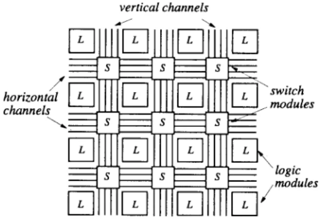
N the symmetrical-array FPGA architecture [1], [8], [20], routing resources consist of horizontal and vertical channels and their intersecting areas. The layout in such an architecture is shown in Fig. 1. An intersecting area of horizontal and vertical channels is referred to as a switch module. A net can change its routing direction via a switch module, and such a direction change requires going through at least one programmable switch inside the switch module. Researchers have shown in [2], [18], and [19] that the feasibility of FPGA design is most constrained by routing resources, and circuit performance in FPGA’s is most limited by routing delays. Thus, switch-module design and routing are of significant importance in the design and use of FPGA’s.Due to the area constraints of switch modules and delay constraints of routing, the number of switches which can be put inside a switch module is usually limited. On the other hand, Manuscript received January 6, 1995; revised November 3, 1996. This work was supported in part by the Texas Advanced Research Program under Grant 003658459 and a DAC design automation scholarship. Preliminary versions of the work reported in this paper were presented at EURO-DAC ’94 [17] and ICCAD ’94 [5]. This paper was recommended by Associate Editor, M. Sarrafzadeh.
S. Thakur is with Synopsys Inc., Mountain View, CA 94043 USA. Y.-W. Chang is with the Department of Computer and Information Science, National Chiao Tung University, Hsinchu, Taiwan 300.
D. F. Wong is with Department of Computer Sciences, University of Texas, Austin, TX 78712 USA.
S. Muthukrishnan is with Lucent Technologies, Murray Hill, NJ 07974 USA.
Publisher Item Identifier S 0278-0070(97)01280-3.
Fig. 1. Symmetrical array architecture.
fewer switches in a switch module would reduce routability. Thus, this presents a problem of designing switch modules to maximize the routability under area and delay constraints. An experimental evaluation of the effect of varying different parameters, like switch-module and connection-module flexi-bilities, on the amount of routing resources needed to complete routing was reported in [3]. This provides an empirical way to choose a routing architecture. In contrast, Zhu et al. in [21] presented an algorithm for switch-module design that generated designs, given a distribution for the nets, that provide good routability. They did it for more general switch-module architectures than [3]. In order to evaluate their designs, they introduced a switch-module-routing problem, which was the key problem for analyzing the routability of a switch module with respect to various routing instances in the provided distribution. This switch-module-routing problem is addressed in this paper.
Informally, the switch-module-routing problem is described as follows. The input is a switch-module description and a sextuple specifying the number of nets that have to pass through the switch module in the six possible directions through the switch module, namely, the four directions that require a 90-degree turn and the two that pass through. The problem is to determine a configuration of the switches in the switch module that allows the specified number of routings. A more formal definition will be given in the next section.
A network flow based algorithm was developed in [21] for the switch-module-routing problem. But the algorithm was approximate in the sense that it overestimated routability. In this paper, we present an optimal algorithm for the problem, based on integer linear programming (ILP). Although the 0278–0070/97$10.00 1997 IEEE
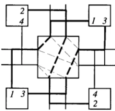
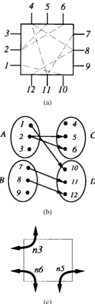
Fig. 2. An infeasible FPGA routing instance.
algorithm, in the worst case, does not run in polynomial time, experimental results consistently show that our algorithm is very efficient for practical-sized switch modules. For exam-ple, running times for all the 20 20 switch modules we considered averaged about 0.25 s of central processing unit (CPU) time. We further improve this approach by proposing a method that avoids having to solve the integer programming problems when actually solving the switch-module-routing problem. This is done by performing some preprocessing on the given switch module. We also identify interesting special cases of the switch-module-routing problem which can be solved optimally in polynomial time. This is achieved by reducing them to instances of bipartite-matching problems and network-flow problems.
Some previous work on FPGA routing [3], [4] suggested that it was a sensible goal for global routers to balance channel densities in all the channels of the FPGA. However, in FPGA’s, the physical architecture of the switch modules con-strains the routing more than channel capacity, as illustrated by the following example.
Example 1: For the switch module and the net specification in Fig. 2, let us suppose the global route for all four nets uses the shown switch module. The density of each channel is two and hence does not exceed the capacity of the channels. Thus, this would be a valid global route if one were concerned about channel density only. Nevertheless, given this global route, the switches available in the switch module do not permit a valid detailed route of all the nets. The thick lines show a feasible detailed route for three of the nets, which is the largest possible number of nets that can be routed through this switch module. Based on our optimal solution for the switch-module-routing problem, we give a way of estimating congestion at individual switch modules in an FPGA. We propose a novel metric for quantifying the congestion level at each switch module in the FPGA. This can be used to generate global-routing paths which avoid heavily congested switch modules. We developed a global router based on this congestion metric. The router was able to route benchmark circuits, consistently using smaller routing resources as compared to a channel-density-guided global router (22% less channel width required for routing completion on an average using Xilinx XC4000-like switch modules on the CGE [4] and SEGA [14] benchmarks).
The rest of the paper is organized as follows. In Section II, we introduce the notation we shall use. Section III gives an ILP-based solution to the switch-module-routing problem
defined formally in the next section. Section IV explores some special cases that can be solved efficiently and optimally. Section V shows how preprocessing can be used to avoid use of ILP at run time. Section VI shows the use of this theory in the development of a global router. Finally, Section VII shows the experimental data.
II. DEFINITIONS ANDPROBLEMSPECIFICATION
A switch module is a rectangular box with
terminals on the left and right faces and terminals on the top and bottom faces. Within a switch module, various terminals are interconnected in some manner dependent on the module. A switch module can be one of two types, namely, a switch matrix or a switch block.
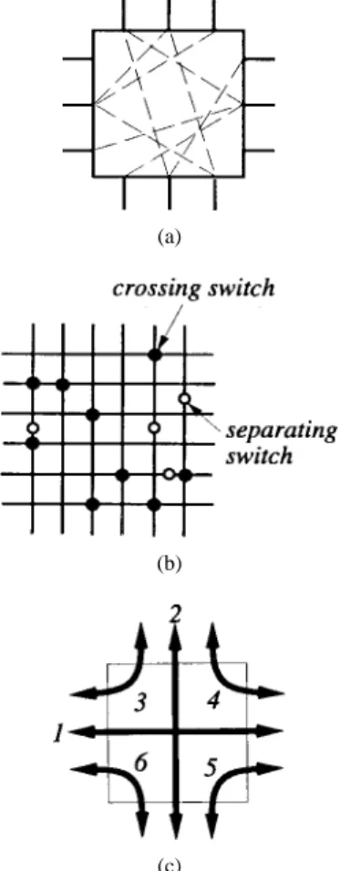
A switch matrix is a rectangular grid of horizontal tracks and vertical tracks. These tracks are electrically noninteracting. The horizontal tracks are numbered top to bottom and the vertical tracks left to right. A switch matrix comprises two types of switches, namely, crossing switches and separating switches. These switches are utilized in estab-lishing connections between the tracks. Crossing switches are found at the intersection of a horizontal track and a vertical track. A crossing switch between a horizontal track and a vertical track has the following property. When on, it connects tracks and electrically. When off, these two tracks are electrically noninteracting. Separating switches are found anywhere along a track, subject to the constraint that each horizontal or vertical track has at most one separating switch. A separating switch on track , when off, splits track into two electrically noninteracting tracks. When on, track becomes a single electrical track. A switch matrix is the specification of the placement of crossing switches and separating switches on a given grid. An example switch matrix is shown in Fig. 3(b).
A switch block is a rectangular box with terminals on the left and right faces and on the top and bottom. Some pairs of terminals on different faces of the box may have programmable electrical links, i.e., these pairs can be programmed to be connected or disconnected. Moreover, these links are electrically noninteracting, unless they share a terminal. The specification of the switch block gives a list of such terminal pairs. An example switch block is shown in Fig. 3(a).
Henceforth, a connection is an electrical path in the switch module between two terminals on different faces of the switch module. Connections can be of six types as shown in Fig. 3(c).
The connection labeled , in Fig. 3(c) is said
to be of Type . Type 1 and Type 2 connections are called straight connections and Types 3, 4, 5, and 6 are called bent connections. For a switch matrix, it is additionally required that at most one switch be found on the electrical path comprising the connection. Thus, only straight connections can use a separating switch. For a switch block, connections have to be chosen from the programmable links specified.
A routing requirement vector ( ) is a sextuple
where ,
(a)
(b)
(c)
Fig. 3. Models for switch module. (a) Switch Block. (b) Switch Matrix. (c) Six types of connections.
module and , a routing is a set of connections which are electrically noninteracting such that there are of Type connections, for . Note that a set of connections are electrically noninteracting only if the terminals on any two paths are distinct. In case of the switch matrices, for the set of connections to be electrically noninteracting, it is additionally required that the paths be disjoint, that is, no two paths share parts of a track. For switch matrices, notice the following role of separating switches. By setting the separating switch on the horizontal track to off, the track to the left is electrically disconnected from the track to the right. Therefore, these two segments can be part of two different connections in any routing. An is said to be routable on a switch module
, if there exists a routing for on .
Example 2: In Fig. 4 a switch matrix and the routing for
the on this switch matrix are shown. The
is not routable on the same switch matrix as only the two crossing switches on vertical track 2 can be used for a Type 3 routing, and both cannot be used simultaneously.
We consider the following problems.
Routing Decision Problem (RDP): Given a switch module (either a switch matrix or a switch block) and an , is routable on ?
Routing Solution Problem (RSP): Given a switch module (either a switch matrix or a switch block) and an , determine a routing for on , if any.
For convenience, we often refer to these problems as simply RDP with or RSP with , omitting the input .
Fig. 4. Example of routing.
III. INTEGER PROGRAMMING FORMULATION
In this section we solve the RDP using an ILP. The solution to the RSP is obtained from the solution to the ILP. We show our formulations for switch matrices and switch blocks separately.
A. Switch Matrix
Consider the RDP with the and switch
matrix . We formulate this problem as an ILP. In the resultant ILP, there are two main sets of constraints. The first set contains at most two constraints for each horizontal or vertical track. For each horizontal track one constraint ensures that the segment of the track to the left of the separating switch, if any, is part of at most one connection. The other constraint ensures this for the segment to the right of the separating switch. Similarly, at most two constraints are generated for each vertical track. Note that if a track does not contain a separating switch, then only one constraint is generated for this track. A set of constraints and an objective function are generated to ensure that a maximum number of connections specified by the are routed in the solution of the ILP. We introduce some notation to succinctly describe the ILP.
Let , and be four constant matrices defined as follows:
if a crossing switch is found between horizontal track and vertical track such that a separating switch, if any, in this horizontal track is to the right of this crossing switch
otherwise
. is similarly constructed as an indicator matrix of the crossing switches to the right of separating switches in the horizontal tracks. Likewise, ( ) is an indicator matrix of the crossing switches above (below) the separating switches in the vertical tracks.
Four variable matrices are as follows: if has a crossing switch between horizontal track and vertical track and this can be used to achieve a connection of Type
otherwise
. Variable is an indicator variable that indicates if the switch between horizontal track and vertical track is utilized in a connection
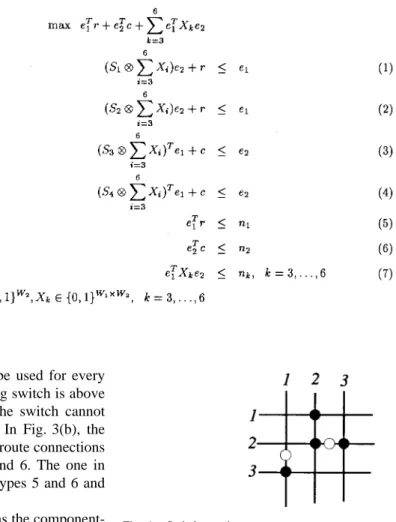
Fig. 5. ILP formulation for switch matrix.
of Type . Note that not every switch can be used for every type of connection. For example, if a crossing switch is above a separating switch for that column, then the switch cannot be used to realize a connection of Type 6. In Fig. 3(b), the crossing switch in row 2, column 1 can only route connections of the Types 3 and 4 and not of Types 5 and 6. The one in row 4, column 1 can route connections of Types 5 and 6 and not of Types 3 and 4.
Define the binary operator on matrices as the
component-wise multiplication, i.e., . Thus, each entry
in is the product of the corresponding entries in and .
Define a variable column vector of dimension as if horizontal track is used in a connection of Type 1
otherwise
for .
Define a variable column vector of dimension as if vertical track is used in a connection of Type 2
otherwise
for .
Let and be two constant column vectors of dimensions and , respectively, with all components one. The integer programming formulation is shown in Fig. 7. In Fig. 5, inequality (1) ensures that the track to the left of the separating switch on each row, if any, are part of at most one connection. Inequality (2) does the same for the track to the right of the separating switch. Similarly, inequalities (3) and (4) ensure that the tracks above and below the separating switch on each column, if any, are part of at most one connection. The objective function, together with the last three inequalities,
guarantees that the is routable if the maximum
Fig. 6. Switch matrix.
value of the objective function is . This will be shown in Theorem 1. The number of variables
number of switches and
the number of constraints
number of switches .
Theorem 1: The problem ILP1 has a solution with objective
value if and only if the is routable
on .
Proof Sketch: If ILP1 has a solution with objective value , then constraints (5)–(7) are satisfied with equality. Since the problem has a solution, the “on” variables give a
way to route using the convention established
before for naming variables. Constraints (1)–(4) ensure that the routing thus generated is valid.
Similarly, if is routable, then there exists an assignment to variables such that the constraints (1)–(4) are satisfied and (5)–(7) are satisfied with equality. Hence, the value of the objective function is .
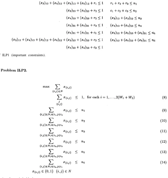
Example 3: Consider the switch matrix in Fig. 6. Fig. 7 shows a set of important constraints in the corresponding ILP. B. Switch Block
Consider an RDP with and switch block .
Fig. 7. Example of ILP1 (important constraints).
Fig. 8. ILP formulation for switch block.
of inequalities. One set of inequalities is used to ensure that every terminal is used at most once. A set of six inequalities with the objective function are used to ensure that the routing generated by the solution to the ILP routes as many of the connections specified by the .
Label the terminals as starting from
the lower most terminal on the left face and proceeding clockwise. The programmable links are specified by sets containing pairs of the terminals they connect. The terminals of a given connection come from different faces, as stated
before. Let there exists a programmable link
between terminals . Let
, ,
and . These sets
identify the terminals of each of the four faces of the switch block. Define a variable for each programmable link . This is a decision variable that is chosen to be one, if the corresponding connection is chosen for the routing, else it is zero. The integer linear program is shown in Fig. 14. The number of variables and number of constraints
.
Theorem 2: The problem ILP2 has a solution with objective
value if and only if the is routable
on .
Proof Sketch: If ILP2 has a solution with objective value , then constraints (9)–(14), shown in Fig. 8, are sat-isfied with equality. Since the problem has a solution, the
“on” variables give a way to route using the
convention established before for naming variables. The first constraint ensures that the routing thus generated is valid, i.e., each terminal is used in at most one connection.
Similarly, if is routable, then there exists an assignment to variables such that the first constraint is satisfied and (9)–(14) are satisfied with equality. Hence, the value of the objective function is .
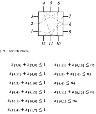
Example 4: A switch block and the corresponding set of important constraints are shown in Figs. 9 and 10, respectively.
IV. SPECIAL CASES
Since the integer-programming problem is NP-complete [7], polynomial time algorithms are not known for RDP and RSP
Fig. 9. Switch block.
Fig. 10. Example of ILP2 (important constraints).
using the approach in Section III. In this section we identify several interesting classes of switch modules for which RDP and RSP can be solved in polynomial time.
Again, for convenience, the cases of switch blocks and switch matrices are considered separately. In what follows, we consider solving the RDP. The solutions to the corresponding RSP’s are directly obtained from the proposed solutions to the RDP.
Define a generic to be a sextuple in which each component is either a number or a special symbol “ .” Any generic represents the class of all ’s which differ only in the components marked “ .”
Example 5: The vector is a generic . The vector , represents the class containing all ’s which have zeros in components 2–5. They may have zeros in components 1 and 6 but that is not necessary. Examples of
’s in this class include and .
In what follows, RDP (or RSP) with generic stands for the problem of RDP on any in the class of ’s represented by .
A. Switch Matrix
Case A—No Separating Switches: Suppose that the given switch matrix contains no separating switches. We char-acterize the complexity of routing on in terms of the complexity of the matching problem. The bipartite-matching problem is to determine if a given bipartite graph has a matching of size [12].
Let and be two problems. We denote if
reduces to , that is, an efficient algorithm for problem yields an efficient algorithm for .1
1Formally, we sayP1 ) P2 if an instance of problem P2 can be reduced
Lemma 1: RDP with RDP with
.
Proof: Consider the instance of RDP on with
. If or the
problem is trivially infeasible. Otherwise
is routable on if and only if is routable
on . This is because, given a routing for ,
we can generate a routing for by utilizing
horizontal tracks and vertical tracks disjoint from the
connections in the routing of .
Lemma 2: RDP with RDP with
.
Proof: We claim that is
routable on a switch matrix if
is routable. We observe that any connection from left to top, in the absence of separating switches, renders the corresponding horizontal and vertical tracks unusable for further connections. Indeed this observation holds for all bent connections. Therefore, a left to top connection can be replaced by any other bent connection without causing any conflicts with the other connections in routing. In particular,
if of Type 3 connections are possible
then we can always replace these with connections of Type . Therefore, if
is routable, so is .
Lemma 3: RDP with bipartite-matching
problem.
Proof: Consider the instance of RDP with . We construct a bipartite graph as
follows. Let be the vertex set where has
a vertex for each terminal on the left face of the switch module and one for each terminal on the top. Thus,
. For every let
if and only if there is a crossing switch between the horizontal track and vertical track . Then, we claim
that, has a bipartite matching of size if and
only if the is routable.
If the is routable then crossing switches have been used in the routing. Choose the corresponding edges in to give a matching of size . Routability criterion ensure that no row or column is used more than once.
If there is a bipartite matching of size in then choose the switches corresponding to the edges in the matching to route connections from the left to the top in the switch module.
To prove the reduction in the other direction, given a
bipartite graph , construct
a switching matrix as follows: place a crossing switch between horizontal track and vertical track if and
only if . We claim that has a matching of size
if and only if the is routable on . The
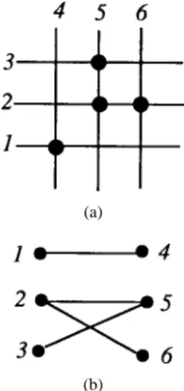
proof is along the lines sketched above; it is omitted here. Example 6: A switch matrix with the bipartite graph in
the transformation of RDP with is shown in
Fig. 11. For any integer , the can be
to an instance of problemP1 in time O(W1+ W2+ jT j) where T is the set of crossing switches inM, and M is the switch matrix in one of the problems
(a)
(b)
Fig. 11. No separating switches. (a) Switch matrix. (b) Bipartite graph.
routed on the switch matrix in Fig. 11(a) if and only if the graph in Fig. 11(b) has a matching of size . It is easy to see
that any yields a routable .
Now we are ready to prove the following theorem.
Theorem 3: RDP with
bipartite-matching problem.
Proof: Trivially, RDP with RDP with
RDP with . Combined with
Lemmas 1, 2, and 3, this yields the theorem.
The bipartite-matching problem can be solved in time for a bipartite graph [12]. From Theo-rem 3, it follows that RDP for a switch matrix with no
sep-arating switches can be solved in time ,
where is the number of crossing switches in . In fact, Theorem 3 implies something stronger: any algorithm for solv-ing RDP on which is faster than time
immediately yields an algorithm for the bipartite-matching
problem which is faster than . Note that the
existence of such an algorithm for the bipartite-matching problem is a long-standing open problem. Therefore,
im-proving the time bound of , for routing
on with no separating switches, is an extremely hard problem.
Let be a switch matrix without separating switches such that the corresponding bipartite graph (see proof of Lemma 3) has a perfect matching. Let be any other switch matrix without separating switches. The following corollary of Theorem 3 is easy to see.
Corollary 1: An is routable on only if it can be
routed on .
This corollary asserts that a switch matrix is the most “powerful” in the class of switch matrices without separating switches. This means that, given , any that can be routed on some switch matrix without separating switches can be routed on . Thus, if the number of crossing switches is taken as a measure of complexity, then designing a switch matrix, for which the corresponding bipartite graph does not have a perfect matching, is, in general, a waste of resource. This fact can be used in the design of a good switch matrix without separating switches.
Fig. 12. Noninterfering network.
Case B—Without Separating Switches in Horizontal or
Ver-tical Tracks: Consider RDP or RSP with .
Assume that in the switch matrix for these problems, the hor-izontal tracks do not contain any separating switches. Similar results hold for the case where vertical tracks do not have sepa-rating switches. Under this condition, it is easy to see using the technique in the proof of Lemma 2 that
is routable if and only if is
routable. The RDP with generic is known
to be solvable using unit-capacity network flows [21]. It follows that under the given condition, RDP or RSP with is solvable as well, using unit-network capacity unit-network flows.
Case C—Class of Problems Solvable by Network Flows: Consider the following problem which we call the noninter-fering network-flow problem, shown in Fig. 12.
Consider a directed network with four blocks of nodes, namely, and . In addition there exist special nodes and , respectively, the pair of source nodes and the pair of sink nodes. Arcs between nodes in the blocks, if any, exist between nodes in block and or and , or between nodes in block and . In particular, there are no arcs between nodes in the same block. The source ( ) is connected to each node in ( ). Every node in ( ) is connected to the sink ( ). Each arc has capacity one. The noninterfering network-flow problem is the following. Given such a network, and integers , and , does there exist a feasible flow such that source supplies a flow of , source supplies a flow of , sink receives a flow of , and sink receives a flow of ? It is easy to see that such a flow exists if and only if there is a matching between the vertex sets and such that there exist exactly arcs between nodes in and , exactly arcs between nodes in and , and exactly arcs between nodes in and . Following are two categories of RDP’s which can be solved using a transformation to the noninterfering network-flow problem. In what follows, the switch matrix is assumed to have the following property. Each horizontal and vertical track of the matrix has precisely one separating switch.
1) RDP’s with generic in which the components corre-sponding to any three bent connections are marked “ ,” and the remaining components are zero. For example,
RDP with .
2) RDP’s with ’s in which the components correspond-ing to any two bent connections which do not share a face of the switch matrix are marked “ ,” and the component of any one straight connection is marked “ .”
(a)
(b)
(c)
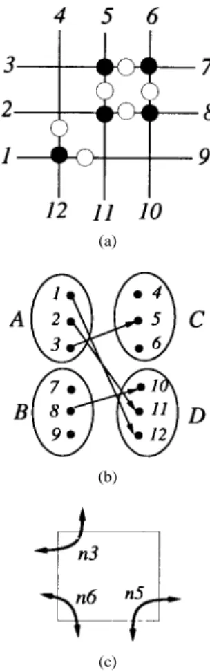
Fig. 13. Example of a transformation into the noninterfering network-flow problem. (a) Switch matrix. (b) Network. (c) Requirements.
The remaining components are zero. For example, RDP
with .
We now sketch the transformations from problems listed above to noninterfering network-flow problems.
Consider an example of a problem in Category 2 above, for
example, RDP with . We create a node for
every terminal of the switch matrix. The nodes of the left face form block , those on the right form , those on the top form , and those on the bottom form . For a crossing switch which is found between the horizontal track and vertical track , create an edge from the node in to the one in corresponding to the terminals and . It is crucial to note that since each horizontal and vertical track has precisely one separating switch, a crossing switch can be utilized in precisely one bent connection. It is now easy to observe that is routable if and only if there is a matching
between the vertex sets and such that there
exist exactly arcs between nodes in and , exactly arcs between nodes in and , and exactly arcs between
nodes in and . Thus, RDP with is
transformed to the noninterfering network-flow problem. Example 7: Fig. 13 gives an example of this transforma-tion. The sources and sinks are omitted for clarity.
A similar construction suffices for transforming a problem in Category 2 above to the noninterfering network-flow problem. Using standard techniques for computing the max-flow in networks [9], the noninterfering network-flow problem on a
network can be solved in time [16].
Therefore, problems in Categories 1 and 2 above can be solved
in time .
B. Switch Block
The problem of routing in switch blocks is, in some sense, simpler than that on switch matrices. This is because connec-tions can interfere with each other if and only if they share a terminal. In the case of a switch matrix, they could additionally interfere if the connections shared a part of a track.
We show a few special cases of routing on switch blocks that have polynomial-time algorithms. The explanations are similar to the corresponding switch matrix cases, and we just give brief ideas about the algorithms or reductions.
Case A—Problems Solvable by Flows in Noninterfering Net-works: The concept of noninterfering networks has been introduced earlier in Section IV-A, Case C. The category of ’s that can be routed on switch blocks using these network-flow techniques is the same as those enumerated in Section IV-A, Case C.
The only difference in the transformation is that only arcs corresponding to relevant programmable links are considered.
For example, for the RDP with , only arcs
corresponding to left to top, right to bottom, and left to bottom programmable links are drawn.
Example 8: An illustration of the above transformation is shown in Fig. 14. The sources and sinks are omitted for clarity. Case B—Problems Solvable by Single Source Network Flows: Consider the case in which the nonzero routing requirements in the share a common face of the switch
block. An example is RDP with generic .
RDP with such ’s can be transformed to a single source network flow problem. We show how to do this for the
RDP with . There is one node for each
terminal. Call the block of nodes corresponding to the left, top, right, and bottom faces , and , respectively. There are four special nodes, a source and three sinks , and . For each node in , there is an arc to a node in if there is a programmable link between the corresponding terminals. Similarly, there are arcs from the nodes in to those in and . There is an arc from to every node in and from each node in , and to , and , respectively. All arcs have capacity one. The problem now is that given such a network, is there a feasible flow where supplies a flow of
and , and receive flows of , and ,
respectively? This can be solved by network-flow algorithms
in time where is the set
of programmable links as in Section III-B [16].
Example 9: An example of this transformation is shown in Fig. 15. The sources and sinks are omitted for clarity.
V. MINIMAL DOMINATING SET
For this section, fix a switch module . Consider solving either RDP or RSP on for various ’s. Using our algorithm in Section III, an instance of integer programming problem is solved for each . In this section, we describe a precom-putation on so that following this precomputation, either
(a)
(b)
(c)
Fig. 14. Example noninterfering network-flow transformation for switch block. (a) Switch block. (b) Network. (c) Requirements.
RDP or RSP on can be solved for any given without resorting to the integer programming problem. For a given , a set of routing requirement vectors are identified during the precomputation. This involves solving several integer programs. Following this computation, RDP or RSP on any given can be solved fast by comparing it with this set of ’s. Both the computation of this set and the comparison of a given with the ’s in this set are now described. First consider solving RDP.
An is said to dominate another
if and only if
and for some . It is a simple observation that any is routable if another is routable on , and dominates . Intuitively, we wish to compute the set of all ’s which dominate all the routable ’s for . We formalize this below.
A set of ’s is called a dominating set for a switch module , if for an , is routable on if and only
if either , or there exists an such that
dominates . A dominating set for is called minimal if
neither dominates nor dominates . The
following property is crucial.
Lemma 4: The minimal dominating set for a switch module is unique.
Proof: Suppose for contradiction that are two dis-tinct minimal dominating sets for . Consider the case when
(a)
(b)
(c)
Fig. 15. Example of a transformation into single source network-flow prob-lem. (a) Switch block. (b) Network. (c) Requirements.
. In this case there exists a such that and . Since is a dominating set, there exists a
that dominates . Since is a dominating set as well, either , or for some , dominates . In either case, there exists an in that dominates . This contradicts the assumption that is minimal. Similarly it can be shown that
if then cannot be minimal.
Observe that the set of routable ’s for is partially ordered under dominance relation. An is called a top element if it is routable and there exists no other that dominates . The following lemma is the key in computing the minimal dominating set for .
Lemma 5: Let is a top element . Then is the minimal dominating set.
Proof: is a dominating set since for any which is not a top element, there exists a top element that dominates it. Also, if and are two top elements, does not dominate , and does not dominate . Therefore, is minimal. By Lemma 4, is the unique minimal dominating set.
Let . Let be the set of ’s for .
Define An is a child
of if , and if differs from
in exactly one component. The is called a parent of .
For , the th parent of is the only parent of
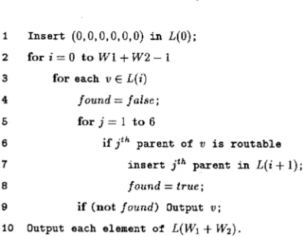
Fig. 16. Algorithm for computing the dominating set.
up to six parents and up to six children. Note that the ’s
and have no children
and no parents respectively.
We describe an algorithm to compute the minimal dominat-ing set for a given switch module . Our algorithm proceeds
in levels . At level , the set of ’s in
is considered. In particular, only those ’s in , all of whose children in are routable, are considered. For each such , using the integer programming approach in Section III, it is determined if the is routable. All the ’s that were considered in level , which have the property that none of their parents in level are routable, are output as top elements. Note that it is sufficient to stop the algorithm after level , since in succeeding levels, the ’s satisfy the trivial infeasibility condition from Section II. From Lemma 5, it is easy to see that the set of top elements in the output of our algorithm is the minimal dominating set. The pseudocode is shown in Algorithm Minimal_Dominating_Set (see Fig. 16).
Computing the minimal dominating set for completes the precomputation. Following this, consider solving RDP with . Clearly, is routable if and only if or there exists some in which dominates . This can be checked quickly by successively performing a binary search on the components of the sextuples in a straightforward manner. Note in particular that no integer programming problem needs to be solved.
To solve RSP, we modify the precomputation described above. Along with each determined to be in the minimal dominating set , we determine and store the routing for . Following this, RSP for any given can be solved fast. First determine if or find an element , if any, in which dominates . In the second case, it is easily seen that a routing for , if any, can be generated from the routing for if exists. Again, no integer programming problem is solved in RSP.
To sum up, by precomputing the minimal dominating set of off-line, the need to solve an integer programming problem while solving RDP or RSP on-line is avoided.
VI. GLOBAL ROUTING
We now show how the minimal dominating set, whose computation has been described in the previous section, can be used in global routing. In this paper we shall limit ourselves to switch modules being switch blocks. A similar approach can be used for switch matrices. Our demonstrative algorithm will closely follow the maze-routing algorithm. A description of the maze-routing approach is given in [13]. We shall model the FPGA as a weighted graph. Paths in the graph will represent routes in the FPGA. The novelty of our approach lies in the way we compute the weights of the graph edges. For this we will propose a new metric that makes use of the minimal dominating set. This metric captures the constraints imposed by the limited switches available in the switch block. We assume that no jogs are used within switch blocks.
For simplicity, we shall assume that all switch modules
in the FPGA are identical and that . This
is the case with most commercially available FPGA’s. The techniques to be described can be easily generalized to avoid making these assumptions.
We first introduce two definitions. We define the switch-block density of a switch switch-block , denoted by , as a vector
, where is the
number of Type connections currently routed through . Let denote the dominating set of each switch block in the FPGA. We define the set
dominates
Thus, is the set of ’s in the dominating set of which dominate . Since the feasibility condition with respect to a switch block can be characterized by its minimal dominating set, we can model congestion as a function of and . The global-routing algorithm is based on a graph search technique guided by the congestion information associated with switch blocks. The router assigns higher costs to route nets through congested areas of the FPGA to balance the net distribution among routing channels. At the end of global routing, we say that a switch block in the FPGA is feasible if is routable on .
A. Modeling the FPGA
Before we can apply the graph search technique to FPGA routing, we first need to model the FPGA as a graph such that the graph topology can represent the FPGA architecture. Fig. 17 illustrates the FPGA modeling. As shown in Fig. 17, each logic block or connection block is represented by a node, each routing channel is modeled as an edge called a channel edge, and each connection between a logic block and a connection block is modeled as an edge called a connection edge. We use six edges and four nodes to model the six possible types of nets routing through a switch block. These six edges are referred to as switch edges. See Fig. 17(b) and (c) for the modeling. Paths in the graph represent global routes on the FPGA and vice versa. Weights associated with edges represent congestion information. Henceforth, we shall denote
(a) (b) (c)
Fig. 17. The FPGA graph modeling. (a) A symmetrical-array FPGA architecture. (b) The switch-block modeling. (c) The FPGA modeling.
(a) (b) (c)
(d) (e)
Fig. 18. Dynamically update congestion information during routing. An illustration in a two-dimensional plane with axesxiandxj. (a) The initial stage. (b) and (c) UpdatedS andDS. (d) Only one vector remains inDS. (e) The state whendS 2 R; DS = .
set is partitioned into , the set of channel edges, , the set of connection edges, and , the set of switch edges. B. The Global Routing Algorithm
The global router is based on a modified Dijkstra’s shortest path algorithm [6]. Unlike the traditional global router which is guided by channel density, our FPGA global router is guided by switch-block density. The main goal is to evenly distribute the nets among routing channels so that the channel width required to route all nets is minimized. The algorithm does the routing net by net. For the net being routed currently, we prefer to route it along uncongested routing regions. For a switch edge , denote the switch block corresponding to by . Similarly, for a channel edge , denote the routing channel corresponding to by .
The cost function that guides the global
routing is defined by
where is a constant. This cost function is used to weight
each of edges in .
Fig. 19. Global-Routing Algorithm.
The whole routing procedure is illustrated in Fig. 18. Given an FPGA , we first construct the graph to model .
Initially, for every switch block in the
FPGA. The cost of every edge in is computed using the function above. See Fig. 18(a) for the initial configuration. After a net is routed, and need to be updated to reflect the additional congestion resulting from the routing of the net. The weights associated with the edges on the route are recomputed using the updated and and the cost function shown above. See Fig. 18(b) and (c) for an illustration of the update. In Fig. 18(c), those ’s which no longer dominate are removed from during the update. The process continues as routing proceeds. Notice that the cardinality of monotonically decreases during the process. We assign a high cost to the switch edges corresponding to the switch block when the set is empty. Essentially, at this stage, , and hence, no more nets can be routed through . This is graphically shown in Fig. 18(e). The last step ensures that a saturated switch block gets low priority while routing further nets. Algorithm FPGA_Global_Routing summarizes the process (see Fig. 19).
TABLE I
RUNNING TIMES FOR ILP METHOD
In contrast, the classical channel-density-based router will assign weights to the graph edges based on the following metric. A description of such a cost function is given in [11].
The cost function that guides such a
method is defined by
where is a constant, and is the density in the
channel , corresponding to the channel edge of the FPGA. The overall strategy is quite similar to the one in Algorithm FPGA_Global_Routing. The difference is that update steps need to update the values of for each channel edge along the newly routed path.
VII. EXPERIMENTAL RESULTS
Our experimental results fall into two parts. In Section VII-A, we demonstrate the improvement in solutions to the RDP and RSP. In Section VII-B, we show the effects of the two metrics and on routing.
A. Results of Using Exact Solutions for RDP and RSP We wrote programs that take in routing problems and switch-module descriptions and generate integer programming problems as described in Sections III-A and III-B. We used a popular integer linear programming code called lp_solve that uses branch-and-bound techniques combined with the simplex algorithm for linear programming to generate integer solutions. We ran the program on a Sun Sparc 1 workstation. We tested the sizes of the problems and running times for both switch-matrix and switch-block models. The results are tabulated in Table I where the second column gives the size of the switch
module ( ), the third gives maximum observed
running time, and the fourth column gives the average running time over 100 experiments. The last three columns give an idea about the size of the ILP. In all cases the RDP was being solved. The fast running time of our algorithms makes our approach an attractive one to use in practice for evaluating designs of switch modules as well as for the application to global routing.
We also compared the routabilities of several switch mod-ules as computed by our exact algorithm with those obtained by the approximate algorithm in [21]. This is shown in Table
TABLE II
COMPARISON WITHAPPROXIMATEALGORITHM
II. All experiments used 100 ’s on the switch modules. The extent of overestimation that results from an approximate algorithm justifies the use of our algorithms. The approximate algorithm was off by about 16%, on an average.
We tested the technique mentioned in Section V. We ob-served a dramatically small search-space size, i.e., the car-dinality of the minimal dominating set. For example, it was observed that for a 10 10 switch-matrix design the cardi-nality of the minimal dominating set was 1254 which is just 0.12% of the possible 10 possible ’s. For a 15 15 switch block of the type to be used in the routing in the next section, the cardinality of the dominating set was 1368. As explained before, a binary search could be used on this set of vectors to test for the routability of a specified .
B. Routing Results
To explore the effects of the two congestion metrics and on routing, we implemented the global-routing algorithms described earlier and then integrated them into the CGE [4] and SEGA [14] detailed routers.
We tested the performance of the metrics on 14 indus-trial benchmark circuits used in [4] and [14]. As mentioned earlier, the new metric uses switch-block capacity as a congestion control parameter while the traditional metric is based on channel density. All benchmark circuits were first routed by the two global routers, one based on the metrics and the other on , using the same net ordering to obtain respective global routes. The global routes were
(a) (b)
Fig. 20. (a) The switch-block architecture (FS= 3). (b) The corresponding switch-block model.
Fig. 21. The connection-block architecture (FC = W; W = 3).
then fed into the CGE/SEGA detailed routers to determine final routing solutions. Notice that the most important concern in the experiment shall be the investigation of the effects of the two metrics. For the purpose of fair comparison, we kept our experimental factors simple. For instance, we used the shortest path-based algorithm to explore the effects, and no optimization such as rip-up and reroute was incorpo-rated.
For FPGA’s, the capacity of a channel is the size of the corresponding side of a switch block, . In our experiments, we used the parameter . The FPGA architectures used in the routing based on the two metrics were identical. The switch block used was similar to that of Xilinx XC4000 series FPGA’s [20]. We refer to the flexibility of a switch block , denoted by , as the number of programmable links connected to a terminal in and that of a connection block, , as the number of tracks that a logic-block pin can connect
to [15]. For the architecture we used , and .
Figs. 20 and 21 illustrate the respective switch-block and connection-block architectures for the case .
We evaluated a metric based on the channel width required for global- and detailed-routing completion by using the metric. Since smaller implies the capability of routing a larger circuit on a given FPGA, a metric leading to a smaller requirement for routing is desirable. As defined before, at the end of global routing, a switch block is feasible if is routable on , i.e., if , or if there exists a such that dominates . The columns “Global routing ( )” in Tables III and IV list the channel widths required for routing all the nets based on the metric or such that all switch blocks are feasible. The columns “Detailed routing ( )” give the channel widths required for routing completion, using the global routes generated from the corresponding metric. The results show that better global-routing topologies, in general, lead to better detailed-routing solutions, and the new metric has better area performance than the traditional metric . An average of 22% channel-width reductions on the 14 CGE/SEGA benchmarks is achieved. Fig. 22 shows the detailed-routing solution for the circuit example 2 with the
parameters , and , using the SEGA
detailed router and the global routes generated by our new metric .
VIII. CONCLUSIONS AND FUTUREWORK
In this paper, we described an integer programming ap-proach to solving a routing problem on switch modules. The problem was originally proposed in [21] as an important part of their approach to switch-module design. Experimental results consistently showed that our algorithm was very efficient for practical-size switch modules. We also identified in this paper several special cases of the problem which reduce to well-known problems and to which polynomial-time algorithms are known.
The techniques proposed provide an efficient way of es-timating congestion at switch modules which can be used in computing good global routes. We demonstrated the success of this scheme by showing that a substantial reduction of channel widths are required as compared to methods guided by channel capacity alone. We propose to extend this method to more general FPGA routing architectures, e.g., the one proposed in [10] and other global-routing approaches, e.g., the Steiner-tree formulation.
TABLE IV
COMPARISON OF THEEFFECTS OF THETWOMETRICS AND ONROUTINGUSING THESEGA ROUTER ANDCIRCUITS.
FROMLEFT TORIGHT:SAME AS INTABLEIII, EXCEPT THAT THESEGA ROUTERWASUSED FORDETAILEDROUTING
Fig. 22. The routing solution for the circuit example 2 with the parameters W = 13; FS = 3, and FC = 13, using the SEGA detailed router and the global routes generated by metric .
ACKNOWLEDGMENT
The authors thank Prof. S. Brown of the University of Toronto for providing them with the CGE and SEGA packages. Also, the authors thank K. Zhu for helpful discussions on several topics in the paper and specifically on the formulation in Section III-B.
REFERENCES
[1] Optimized Reconfigurable Cell Array (ORCA) Series Field-Programmable Gate Arrays. AT&T Microelectronics, Advance Data Sheet, Feb., 1993.
[2] N. Bhat and D. Hill, “Routable technology mapping for LUT FPGA’s,” in Proc. Int. Conf. Computer Design, VLSI Computers Processors, 1992, pp. 95–98.
[3] S. Brown, R. J. Francis, J. Rose, and Z. G. Vranesic, Field-Programmable Gate Arrays. Norwell, MA: Kluwer, 1992.
[4] S. Brown, J. Rose, and Z. G. Vranesic, “A detailed router for field-programmable gate arrays,” IEEE Trans. Computer-Aided Design, vol. 11, pp. 620–627, 1992.
[5] Y.-W. Chang, S. Thakur, K. Zhu, and D. F. Wong, “A new global routing algorithm for FPGA’s,” in IEEE/ACM Proc. Int. Conf. Computer-Aided Design, 1994, pp. 380–385.
[6] E. Dijkstra, “A note on two problems in connection with graphs,” Numer. Math., vol. 1, pp. 269–271, 1959.
[7] M. Garey and D. S. Johnson, Computers and Intractability: A Guide to the Theory of NP-Completeness. San Francisco, CA: Freeman, 1979. [8] H.C. Hsieh, W. Carter, J. Ja, E. Cheung, S. Schreifels, C. Erickson,
P. Freidin, L. Tinkey, and R. Kanaza, “Third-generation architecture boosts speed and density of field-programmable gate arrays,” in Proc. IEEE Custom Integrated Circuits Conf., 1990, pp. 31.2.1–31.2.7. [9] T. C. Hu, Integer Programming and Network Flows. Reading, MA:
Addison-Wesley, 1969.
[10] K. Kawana, H. Keida, M. Sakamoto, K. Shibata, and I. Moriyama, “An efficient logic block interconnect architecture for user-reprogrammable gate array,” in Proc. IEEE Custom Integrated Circuits Conf., 1990, pp. 31.3.1–31.3.4
[11] E. S. Kuh and M. Marek-Sadowska, “Global routing,” in Layout Design and Verification, T. Ohtsuki, Ed. Amsterdam, The Netherlands: Elsevier, 1985.
[12] C. Papadimitriou and K. Steiglitz, Combinatorial Optimization-Algorithms and Complexity. Englewood Cliffs, NJ: Prentice-Hall, 1982.
[13] M. J. Lorenzetti and D. S. Baeder, “Routing,” in Physical Design Automation of VLSI System, B. Preas and M. J. Lorenzetti, Eds. Menlo Park, CA: Benjamin-Cummings, 1988.
[14] G. Lemieux and S. Brown, “A detailed routing algorithm for allocating wire segments in field-programmable gate arrays,” in Proc. ACM/SIGDA Physical Design Workshop, Lake Arrowhead, CA, 1993, pp. 215–226. [15] J. Rose and S. Brown, “Flexibility of interconnection structures for
field-programmable gate arrays,” IEEE J. Solid State Circuits, vol. 26, no. 3, pp. 277–282, 1991.
[16] D. D. Sleator and R. E. Tarjan, “A data structure for dynamic trees,” J. Comput. Syst. Sci., vol. 26, pp. 362–391, 1983.
[17] S. Thakur, D. F. Wong, and S. Muthukrishnan, “Algorithms for FPGA switch module routing,” in Proc. European Design Automation Conf., 1994, pp. 265–270.
[18] S. Trimberger, Ed., Field-Programmable Gate Array Technology. Nor-well, MA: Kluwer, 1994.
[19] S. Trimberger and M. Chene, “Placement-based partitioning for lookup-table-based FPGA’s,” in Proc. Int. Conf. Computer Design, VLSI Com-puters Processors, 1992, pp. 91–94.
[20] The Programmable Logic Data Book, Xilinx Inc., 1994.
[21] K. Zhu, D. F. Wong, and Y.-W. Chang, “Switch module design with application to two-dimensional segmentation design,” in Proc. IEEE/ACM Int. Conf. Computer-Aided Design, 1993, pp. 481–486
Murray Hill, NJ, and during the summer of 1995, he was at Synopsys Inc. Presently, he is a Senior Research and Development Engineer at Synopsys Inc., Mountain View, CA. His research interests include algorithms, combinational optimization, logic synthesis, and physical design of VLSI circuits.
Yao-Wen Chang (S’95–A’96) received the B.S. degree in computer science and information engi-neering from National Taiwan University, Taiwan, R.O.C., in 1998 and the M.S. and Ph.D. degrees in computer science from the University of Texas, Austin, in 1993 and 1996, respectively.
He was a Second Lieutenant during his compul-sory military service from 1998 to 1990, a Research Assistant at the Institute of Information Science, Academia Sinica, Taiwan, R.O.C., from 1990 to 1991, and a Teaching/Research Assistant in the Department of Computer Sciences, University of Texas, Austin, from 1992 to 1996. During the summer of 1994, he was with IBM J. Watson Research Center, Yorktown Heights, NY, in the VLSI group. Since 1996, he has been an Associate Professor in the Department of Computer and Information Science, National Chiao Tung University, Hsinchu, Taiwan, R.O.C. His current research interests lie in design automation, architectures, and systems for VLSI and combinatorial optimization.
Dr. Chang received Best Paper Award at the 1995 IEEE International Conference on Computer Design (ICCD ’95).
D. F. Wong received the B.Sc. degree in mathemat-ics from the University of Toronto, Toronto, Canada, the M.S. degree in mathematics from the University of Illinois, Urbana-Champaign, and the Ph.D. degree in computer science from the University of Illinois, Urbana-Champaign, in 1987.
He is currently an Associate Professor of Com-puter Sciences at the University of Texas, Austin. He has published more than 120 technical papers. He is a coauthor of Simulated Annealing for VLSI Design (Norwell, MA: Kluwer, 1998). His main research interest is computer-aided design of VLSI.
Dr. Wong received Best Paper Awards at DAC-86 and ICCD-95 for his work on floorplan design and FPGA routing, respectively. He has served on the program committees of a number of VLSI CAD conferences (e.g., ICCAD, ED&TC, FPGA Symposium, and PD Symposium). He is an Editor of IEEE TRANSACTIONS ONCOMPUTERS.
S. Muthukrishnan received the B.Tech. (Hons.) degree in computer science from the Indian Institute of Technology, Kharagpur, India, in 1989 and the M.S. and Ph.D. degrees from New York University, New York, in 1991 and 1994, respectively, all in computer science.
He was a Postdoctoral Visitor at DIMACS, Rut-gers University, from 1994 to 1995 and on the faculty of University of Warwick, Coventry, UK, from 1995 to 1996. At present, he is a Member of the Technical Staff, Bell Laboratories, Lucent Technologies, Murray Hill, NJ.