國立高雄大學應用數學研究所
碩士論文
利用延拓法解非線性薛丁格方程式
A continuation method for nonlinear Schrödinger
equation
研究生:林怡君撰
指導教授:郭岳承
致謝
首先要感謝我的指導教授郭岳承老師,因為老師總是很有耐心的指導,並且 給予適當的建議,讓我能順利的完成論文。再來要感謝我親愛的父母,謝謝你們 總是為我加油打氣,時時關心我的生活,也一直都給我最大的支持,讓我感到無 比安心的力量。 在這兩年當中,和我一起度過碩士生涯的所有同學們,謝謝你們的陪伴,特 別是怡翔的鼓勵總是讓人感到窩心。還有其他同樣關心著我的朋友們,無論你們 身在何方,有了貼心的話語打氣,也都讓我心裡倍感溫暖,謝謝你們。最後,再 次謝謝我的師長們,以及親愛的家人朋友們,謝謝你們!A continuation method for nonlinear
Schrödinger equation
by
I-Chun Lin
Advisor
Yueh-Cheng Kuo
Department of Applied Mathematics,
National University of Kaohsiung
Kaohsiung, Taiwan 811, R.O.C.
July 2009
Contents
1. Introduction 1
2. Nonlinear Schrödinger equation 2
3. Discretization 4
4. Continuation method 10
4.1 Fixed point iteration method..………..…………...10
4.2 Standard continuation method….………12
4.3 Quotient transformation invariant continuation method .………...16
4.4 Algorithm……….………...………21
5. Numerical results 22
利用延拓法解非線性薛丁格方程式
指導教授:郭岳承 博士 國立高雄大學應用數學所 學生:林怡君 國立高雄大學應用數學所 摘要 在這篇論文中,我們介紹逼近非線性薛丁格方程式的解曲線所用的延拓法。我們探 討離散非線性薛丁格方程式的過程,並且介紹了固定點迭代法和延拓法的概念。我們將 使用商的不變性轉換延拓法去克服一些標準延拓法所產生的問題。最後,會呈現一些數 值上的結果。 關鍵字:延拓法,非線性薛丁格方程式,固定點迭代法,商的不變性轉換A continuation method for nonlinear Schrödinger
equation
Advisor: Dr. Yueh-Cheng Kuo Institute of Applied mathematics National University of Kaohsiung
Student: I-Chun Lin Institute of Applied mathematics National University of Kaohsiung
ABSTRACT
In this thesis, we introduce the continuation method which approximates the solution curve of a nonlinear Schrödinger equation. We study the process of discretizing a nonlinear Schrödinger equation. And we introduce the conception of fixed point iteration method and continuation method. We will use the quotient transformation invariant continuation method so as to overcome some problems of standard continuation method. Eventually, we will show some numerical results.
Keywords: continuation method, nonlinear Schrödinger equation, fixed point iteration
method, quotient transformation invariant
1
Introduction
In this thesis, we consider the solution of a nonlinear Schr¨odinger equation [1]:
−∆qu(x) + α1|u(x)|2u(x) = λ1u(x), (1.1)
for x ∈ Ω and u : Ω → C with normalized constraint Z
Ω
|u(x)|2dx = 1, (1.2)
where Ω ⊆ R2 is a bounded domain, and the Dirichlet boundary condition
u(x) = 0, x ∈ ∂Ω. (1.3) According to [1], we define ∇ = (∂x, ∂y)>, ∇q = ∇ + iγq, −∆q = < ∇q, ∇q >, (1.4) where q = (q1, q2)> represents a vector on Ω , and γ is the magnitude of
magnetic field. From equation (1.4), we can get
−∆q =< ∇q, ∇q >
=< ∇ + iγq, ∇ + iγq >
=< ∇, ∇ > + < iγq, ∇ > + < ∇, iγq > + < iγq, iγq >
= −∆ + iγ∇∗q − iγq∗∇ + γ2q∗q, (1.5)
where ∆q is magnetic laplacian operator[2, 3].
In section 2, we introduce the nonlinear Schr¨odinger equation. We put
uc = u1+ iu2 into equation (1.1). We can get the new equation. To consider
the energy functional and the eigenvalue, we can find the relation between them. After verifying the relation, we want to transform continuous differ-ential equation to discrete equation in section 3. As a result, we use finite difference method to approximate the solution. In other words, we have to discretize the new equation. We can see details in section 3. Now, we have the discrete nonlinear Schr¨odinger equation. We denote the discrete equation as G(u(s), γ(s)) = 0, where s is an arc length parameter.
We use the fixed point iteration method in subsection 4.1 so as to obtain the initial solution of the discrete equation. Then, we use the continuation method to approximate the solution curve. We will explain the conception of standard continuation method in subsection 4.2. Continuation method
includes predictions and corrections. In the part of predictions, we have to find the tangent vector of possible solution on solution curve. Here, we differentiate the discrete equation with respect to s. Then, we can get the system as follows. £ Gu Gγ ¤· ˙u(s) ˙γ(s) ¸ = 0.
By solving the system above, we can obtain the tangent vector. We suppose that (u0, γ0) is the initial solution. And we denote (ui, γi) as the possible
solution. After computing, we can get the new point (u(1)i , γi(1)) in predictions. We continue to discuss the part of corrections. The main idea is Newton’s method. We consider the plane Ni whose normal vector is equal to the
tangent vector. We hope that the point (u(1)i , γi(1)) can converge to (ui, γi)
on the plane Ni iteratively. There are some problems on the computing
process. In order to solve those problems, we have to introduce the idea about the rotation invariance. The solution set contains transformation invariant solution. Hence, we concentrate on solving the quotient solution. As a result, we will develop the quotient invariant transformation continuation method in subsection 4.3. We will add a plane to the system which we have to solve. And we can obtain the meaningful vectors of predictions. We also introduce a small skill on computing so as to overcome some disadvantages. In subsection 4.4, we show the algorithm of continuation method. Eventually, we can get the approximate solution curve by repeating the steps of continuation method. We can see that the numerical results in section 5. And we have a conclusion in section 6.
2
Nonlinear Schr¨
odinger Equation
We use q = · −r cos θ r sin θ ¸ ρ, where ρ = 0 if r < ², 1 + cos(5π ar + π) 2 if ² ≤ r ≤ a, 1 if r ≥ a.
We substitute equation (1.5) into equation (1.1). Then, we can get [−∆ + iγ(∇∗q − q∗∇) + γ2kqk2+ α1|u|2]u = λ1u. (2.1)
We let uc= u1+ iu2, where u1, u2 : Ω → R. Then we can obtain
[−∆ + γ2kqk2+ α1(u21+ u22)]u1− γ(∇∗q − q∗∇)u2 = λ1u1,
[−∆ + γ2kqk2+ α
1(u21+ u22)]u2+ γ(∇∗q − q∗∇)u1 = λ1u2. (2.2)
We rewrite equation (2.1) into below form.
−∆u + iγ∂θ1u + V u + α1|u|
2u = λ
1u. (2.3)
The energy functional [7, 8, 9] is
E(φ) = Z Ω (|∇φ|2+ iγφ∗∂θ1φ + V φ 2+1 2α1|φ| 4). (2.4)
Let equation (2.3) be multiplied by u∗. Then we can get equation as
following.
−u∗∆u + iγu∗∂θ1u + u
∗V u + α
1u∗|u|2u = λ1u∗u. (2.5)
To integrate equation (2.5), it will become Z
(−u∗∆u + iγu∗∂
θ1u + u ∗V u + α 1u∗|u|2u) = Z λ1u∗u. (2.6) Here, − Z u∗∆u = − µ u∗∇u| ∂Ω− Z ∇u · ∇u ¶ = Z |∇u|2. (2.7)
We put equation (2.7) into equation (2.6). From equation (1.2), we can get R u∗u = 1. Equation (2.6) can be represented as
Z
(|∇u|2+ iγu∗∂
θ1u + u
∗V u + α
1u∗|u|2u) = λ1 (2.8)
Comparing the energy funtional E(φ) to eigenvalue λ1 from equations (2.4)
and (2.8), we can find that E(φ) = λ1 −
α1
2 Z
3
Discretization
In this section, we concern about the process of discretization. In order to transform continuous differential equations into discrete equations, we intro-duce finite difference method [4] to approximate the solutions of equations (2.2), (1.2) and (1.3). First, we divide the solutions into grids of nodes. The domain Ω which we consider is a disc. We cut the disc into n radial parts and m azimuthal parts. We let ∆r = 2
2n + 1, ∆θ = 2π
m. And we define the
grid points as below.
ri = (i −
1
2)∆r, i = 1, 2, · · · , n,
θj = (j − 1)∆θ, j = 1, 2, · · · , m.
Here, we see an example for n = 3 and m = 10. We show the discrete points on the domain which is a disc in Figure 1.
1,1 u 1,2 u 1,3 u 1,4 u 1,5 u 1,6 u 1,7 u 1,8 u u1,9 1,10 u 2,1 u 2,2 u 2,3 u 2,4 u 2,5 u 2,6 u 2,7 u 2,8 u u2,9 2,10 u 3,1 u 3,2 u 3,3 u 3,4 u 3,5 u 3,6 u 3,7 u 3,8 u u3,9 3,10 u 1 2 r ∆ r ∆ ∆r ∆r θ ∆ Figure 1: Discretization
We use the coordinate transformation to convert Cartesian coordinate system (x, y) into the polar coordinate system (r, θ). Therefore, we can obtain −∆u = −(uxx + uyy) = −(urr+ 1 rur+ 1 r2uθθ). (3.1)
Now, we first consider the approximate solution of −∆u. We consider lapla-cian operator on disc with Dirichlet conditions as following:
½
−∆u = f (r, θ),
u(r, θ) = C(r, θ), (3.2)
where (r, θ) ∈ Ω.
Next, we replace laplacian by central difference formula as following
urr =
u(ri+1, θj) − 2u(ri, θj) + u(ri−1, θj)
∆r2
ur =
u(ri+1, θj) − u(ri−1, θj)
2∆r
uθθ =
u(ri, θj+1) − 2u(ri, θj) + u(ri, θj−1)
∆θ2 . (3.3)
Then, we substitute equation (3.3) into equations (3.1) and (3.2). We get
− [ 1
∆r2(u(ri+1, θj) − 2u(ri, θj) + u(ri−1, θj)) +
1
2ri∆r
(u(ri+1, θj) − u(ri−1, θj))
+ 1
r2
i∆θ2
(u(ri, θj+1) − 2u(ri, θj) + u(ri, θj−1))] = f (ri, θj). (3.4)
In order to simplify equation (3.4), we rewrite u(ri, θj) to ui,j and f (ri, θj)
to fi,j. And we substitute ri = (i − 12)∆r into equation (3.4). Then, we can
obtain the following
− 1
∆r2[(ui+1,j− 2ui,j+ ui−1,j) +
1
2(i −12)(ui+1,j− ui−1,j) + 1
(i −122)∆θ2(ui,j+1− 2ui,j+ ui,j−1)] = fi,j.
Let ci = 1 2(i −1 2) , di = 1 (i − 1 2)2∆θ2
. Now, we can get the following:
(i, j) fi,j (1, 1) − 1 ∆r2[(−2 − 2d1)u1,1+ d1u1,2+ d1u1,0+ (1 + c1)u2,1+ (1 − c1)u0,1] = f1,1 (1, 2) − 1 ∆r2[(−2 − 2d1)u1,2+ d1u1,3+ d1u1,1+ (1 + c1)u2,2+ (1 − c1)u0,2] = f1,2 (1, 3) − 1 ∆r2[(−2 − 2d1)u1,3+ d1u1,4+ d1u1,2+ (1 + c1)u2,3+ (1 − c1)u0,3] = f1,3 (1, 4) − 1 ∆r2[(−2 − 2d1)u1,4+ d1u1,5+ d1u1,3+ (1 + c1)u2,4+ (1 − c1)u0,4] = f1,4 .. . ... (1, m − 1) − 1 ∆r2[(−2 − 2d1)u1,m−1+ d1u1,m+ d1u1,m−2+ (1 + c1)u2,m−1+ (1 − c1)u0,m−1] = f1,m−1 (1, m) − 1 ∆r2[(−2 − 2d1)u1,m+ d1u1,1+ d1u1,m−1+ (1 + c1)u2,m+ (1 − c1)u0,m] = f1,m
(2, 1) − 1 ∆r2[(−2 − 2d2)u2,1+ d2u2,2+ d2u2,0+ (1 + c2)u3,1+ (1 − c2)u1,1] = f2,1 (2, 2) − 1 ∆r2[(−2 − 2d2)u2,2+ d2u2,3+ d2u2,1+ (1 + c2)u3,2+ (1 − c2)u1,2] = f2,2 (2, 3) − 1 ∆r2[(−2 − 2d2)u2,3+ d2u2,4+ d2u2,2+ (1 + c2)u3,3+ (1 − c2)u1,3] = f2,3 (2, 4) − 1 ∆r2[(−2 − 2d2)u2,4+ d2u2,5+ d2u2,3+ (1 + c2)u3,4+ (1 − c2)u1,4] = f2,4 .. . ... (2, m − 1) − 1 ∆r2[(−2 − 2d2)u2,m−1+ d2u2,m+ d2u2,m−2+ (1 + c2)u3,m−1+ (1 − c2)u1,m−1] = f2,m−1 (2, m) − 1 ∆r2[(−2 − 2d2)u2,m+ d2u2,1+ d2u2,m−1+ (1 + c2)u3,m+ (1 − c2)u1,m] = f2,m .. . ... (n, 1) − 1 ∆r2[(−2 − 2dn)un,1+ dnun,2+ dnun,0+ (1 + cn)un+1,1+ (1 − cn)un−1,1] = fn,1 (n, 2) − 1 ∆r2[(−2 − 2dn)un,2+ dnun,3+ dnun,1+ (1 + cn)un+1,2+ (1 − cn)un−1,2] = fn,2 (n, 3) − 1 ∆r2[(−2 − 2dn)un,3+ dnun,4+ dnun,2+ (1 + cn)un+1,3+ (1 − cn)un−1,3] = fn,3 (n, 4) − 1 ∆r2[(−2 − 2dn)un,4+ dnun,5+ dnun,3+ (1 + cn)un+1,4+ (1 − cn)un−1,4] = fn,4 .. . ... (n, m − 1) − 1 ∆r2[(−2 − 2dn)un,m−1+ dnun,m+ dnun,m−2+ (1 + cn)un+1,m−1+ (1 − cn)un−1,m−1] = fn,m−1 (n, m) − 1 ∆r2[(−2 − 2dn)un,m+ dnun,1+ dnun,m−1+ (1 + cn)un+1,m+ (1 − cn)un−1,m] = fn,m
Then, we want to solve above difference equations related to Dirichlet boundary conditions u(r, θ) = c(r, θ). That is, we solve the linear system of Au = b. We get un+1,1 = cn+1,1 from equation (3.2) and 1 − c1 = 1 −
1 2(1 − 1 2) = 0. The matrix is A = − 1 ∆r2 −2I − d1ψ (1 + c1)I (1 − c2)I −2I − d2ψ (1 + c2)I . .. . .. . .. (1 − cn−1)I −2I − dn−1ψ (1 + cn−1)I (1 − cn)I −2I − dnψ nm×nm , where ψ = 2 −1 −1 −1 2 −1 . .. ... ... −1 2 −1 −1 −1 2 m×m .
b = b1 ... bn−1 bn nm×1 where bi = fi,1 ... fi,m m×1 with i = 1, 2, · · · , n − 1, and bn= 1 ∆r2(1 + cn)Cn+1,1+ fn,1 ... 1 ∆r2(1 + cn)Cn+1,m+ fn,m m×1 .
Now, we use the same steps to discreticize ∇∗q − q∗∇, γ2kqk2 and α 1|u|2. • ∇∗q − q∗∇ x = r cos θ, cos θ = x r; y = r sin θ, sin θ = y r. (3.5) q = µ q1 q2 ¶ = ρ µ −y x ¶ . (3.6) (ρy)∗ = ρy, (ρx)∗ = ρx. (3.7) We use equations (1.4), (3.5), (3.6) and (3.7) to compute ∇∗q − q∗∇.
∇∗q − q∗∇ = · ∂x ∂y ¸∗· q1 q2 ¸ − · q1 q2 ¸∗· ∂x ∂y ¸ , = £ ∂∗ x ∂y∗ ¤· q1 q2 ¸ −£ q∗ 1 q2∗ ¤· ∂x ∂y ¸ , = −£ q∗ 1 q2∗ ¤· ∂x ∂y ¸ , = −£ q∗ 1 q2∗ ¤ 1 r · r cos θ − sin θ r sin θ cos θ ¸ · ∂r ∂θ ¸ , = −1 r £ q∗
1r cos θ + q2∗r sin θ q∗1(− sin θ) + q∗2(cos θ)
¤· ∂r ∂θ ¸ , = −1 r £ (−ρy)∗x + (ρx)∗y (−ρy)∗(−y r) + (ρx)∗( x r) ¤· ∂r ∂θ ¸ , = −1 r £ 0 ρr(x2+ y2) ¤ · ∂r ∂θ ¸ = −1 r £ 0 ρr ¤ · ∂r ∂θ ¸ = −ρ · ∂θ = ∂θ1.
We use the central difference formula as following
uθ =
ui,j+1− ui,j−1
2∆θ . After computing, we can get
Dθ = 1 2∆θ T T . .. T nm×nm , where T = 0 1 −1 0 1 . .. ... ... −1 0 1 −1 0 n×n . And we use
ρi,j : ρi,1 = ρi,2 = · · · = ρi,m= ρi; i = 1, 2, · · · , n.
Hence, the discrete matrix of ∇∗q − q∗∇ is
−ρDθ = − 1 2∆θ T1 T2 . .. Tn nm×nm , where Ti = 0 ρi −ρi 0 ρi . .. ... ... −ρi 0 ρi −ρi 0 n×n , i = 1, 2, · · · , n. • γ2kqk2
By equation (3.6), we can get q2
1+ q22 = ρ2(y2+ x2) = ρ2· r2. The discrete
matrix of γ2kqk2 can be represented as following
γ2· D q = γ2 Q1 Q2 . .. Qn nm×nm ,
where Qi = q2 1(ri, θ1) + q22(ri, θ1) q2 1(ri, θ2) + q22(ri, θ2) . .. q2 1(ri, θm) + q22(ri, θm) n×n , = ρ2 iri2 ρ2 ir2i . .. ρ2 iri2 n×n , i = 1, 2, · · · , n. • α1|u|2
We use the same steps to discreticize the operator α1|u|2 = α1(u21 + u22).
The matrix is α1 · U = α1· U1 U2 . .. Un nm×nm , where Ui = u2 1(ri, θ1) + u22(ri, θ1) u2 1(ri, θ2) + u22(ri, θ2) . .. u2 1(ri, θm) + u22(ri, θm) n×n , i = 1, 2, · · · , n. • RΩ|u(x)|2dx = 1
By using formula for area of sector 1
2∆r2∆θ, we can get as following
i = 1 1 2 µ 1 2∆r ¶2 ∆θ = 1 2∆r 2∆θ · 1 4, i = 2 1 2∆r 2∆θ "µ 3 2 ¶2 − µ 1 2 ¶2# = 1 2∆r 2∆θ · 2, ... ... i = n 1 2∆r 2∆θ "µ (2i − 1) 2 ¶2 − µ 2(i − 1) − 1 2 ¶2# = 1 2∆r 2∆θ · 2(i − 1).
Hence, we obtain the discrete matrix is C>· U0 = 1. C>= 1 2∆r2∆θ £ 1 4 · · · 14 2 · · · 2 · · · 2(i − 1) · · · 2(i − 1)) ¤ , U0 = ¯ U1 ... ¯ Un , where ¯Ui = u2 1(ri, θ1) + u22(ri, θ1) ... u2 1(ri, θm) + u22(ri, θm) with i = 1, 2, · · · , n. Finally, the discrete nonlinear Schr¨odinger equation relative to equation (2.3) can be represented as
A1uc+ iγSuc+ α1u¯c◦ u°c2 = λ1uc, C>(¯u
c◦ uc) = 1. (3.8)
In (3.8), A1 is the discrete matrix for the operator of −∆ + V . S is the
discrete matrix for the operator of ∂θ1 and S is a skew-symmetric matrix. We
denote ◦ as Hadamard product. We can find that C>(¯u
c◦ uc) will be pure
imaginary. Therefore, we can get u°2
c = uc◦uc, u°12 = u1◦u1 and u°22 = u2◦u2.
We also can obtain the energy functional corresponding to (2.4) is
E(φ) = C>(¯u c◦ A1uc+ iγ ¯uc◦ Suc+ α1 2 u¯ °2 c ◦ u°c2 ).
4
Continuation Methed
4.1
Fixed point iteration method
Now, we want to get the initial solution of equation (3.8). Hence, we use fixed point iteration method [6] so as to converge the solution. We let uc= u1+iu2,
where u1,u2 ∈ RN and N = n · m. And we put it into equation (3.8). Then,
we can rewrite equation (3.8) into the form as follows. (A1 + α1U)u1− γSu2 = λ1u1,
(A1 + α1U)u2+ γSu1 = λ1u2,
C>U0 = 1. (4.1)
We let γ = 0. The equations (4.1) will become the form as below. (A + α1U)u1 = λ1u1,
(A + α1U)u2 = λ1u2,
C>U0
= 1. (4.2)
Then, we let u2 = 0. Equations (4.2) can be simplified as
C>u°2
1 = 1. (4.3b)
Now, we consider the eigenvalue problem of equation (4.3a). First, we let u(0) ∈ RN be a random vector. We choose c
1 = C> · u(0)
°2
such that
u(0) = √1
c1u
(0). u(0) will satisfy equation (4.3b), that is,
C>u(0)°2 = C>1 c1 u(0)°2 = C> 1 C>u(0)°2 u (0)°2 = 1.
Next, we substitute equation above into equation (4.3a). To solve the eigenvalue problem, we can obtain eigenvalues and eigenvectors. We choose the smallest eigenvalue λ(1)1 and corresponding eigenvector u(1)1 and let u(1)1 satisfy equation (4.3b). Repeating solving the eigenvalue problem iteratively, we can get λ(i)1 and u(i)1 . Finally, we stop the iterations until the eigenvalue converges. In other words, it means that ku(i)1 − u(i+1)1 k < Tolerance. When
the eigenvectors satisfy the condition of convergence, we can get solutions which we need. We suppose the iteration number is k. Hence, we use u(k)1 and λ(k)1 to denote convergent solutions. After computing above, we obtain a initial solution:
(u1, u2, λ1, γ) = (u(k)1 , u2, λ(k)1 , 0),
where u(k)1 ∈ RN and u
2 is a zero vector ∈ RN and λ(k)1 , 0 ∈ R1. • Algorithm Step 1. u(0) =rand(N, 1) Let u(0) = √1 c1u (0), then C>u(0)°2 = 1. Step 2. Set i = 0. Compute (A + α1u(i) °2 )u(i+1) = λ minu(i+1). Let u(i+1) = c
1u(i+1) such that C>u(i+1)
°2
= 1. Step 3.
If ku(i)− u(i+1)k <Tol, then Stop.
Step 4. Set i = i + 1. Go to Step 2.
4.2
Standard Continuation Method
In this section, we introduce the process of standard continuation method [5]. We use continuation method approximating to the solution curve. Mainly, we concentrate on solving the system as following
G(u, γ) = 0, (4.4)
and we let G = (G1, G2, G3) where
G1(u, γ) = (A1+ α1U)u1 − γSu2− λ1u1,
G2(u, γ) = (A1+ α1U)u2 + γSu1− λ1u2,
G3(u, γ) = C>U 0
− 1,
and G : R2N +2 → R2N +1.
Hence, we can find that the Jacobian of G(u, γ) is derived from the
G(u, γ). We denote the Jacobian of G(u, γ) as JG(u, γ) = [Gu, Gγ] ∈ R(2N +1)×(2N +2).
We can see that
Gu = ∂G1 ∂u1 ∂G1 ∂u2 ∂G1 ∂λ1 ∂G2 ∂u1 ∂G2 ∂u2 ∂G2 ∂λ1 ∂G3 ∂u1 ∂G3 ∂u2 ∂G3 ∂λ1 = ¯ A + α1(3u°12 + u° 2 2 ) 2α1(u1◦ u2) − γS −u1 2α1(u1◦ u2) + γS A + α¯ 1(3u°22 + u° 2 1 ) −u2 2C>◦ u> 1 2C>◦ u>2 0 ∈ R(2N +1)×(2N +1), where ¯A = A1− λ1IN ×N = A + γ2Dq− λ1IN ×N. Gγ = ∂G1 ∂γ ∂G2 ∂γ ∂G3 ∂γ = 2γ (q 2 1+ q22) ◦ u1 (q2 1+ q22) ◦ u2 0 + −SuSu12 0 ∈ R(2N +1)×1. And we let u = (u>
1, u>2, λ1)> ∈ R2N +1. The continuation method includes
the predictions and corrections. We denote (u0, γ0)> as the initial solution,
where u0 = (u>10, u
>
20, λ10). And the arc length s is the parameter of the
solution curve.
First, we want to compute the unit tangent vector ~p0 = ( ˙u>0, ˙γ0)> of
the initial solution on the solution curve, where ˙u>
0 = ( ˙u>10, ˙u
>
20, ˙λ10). Then,
we get a point (u(1)1 , γ1(1))> = (u
0, γ0)> + ¯s~p0 where ¯s is the step length.
Next, we consider a plane N1 which contains the point (u(1)1 , γ (1)
1 )>. And the
of the plane N1 and solution curve. We denote (u1, γ1)> as the point of
intersection. Finally, in order to let (u(1)1 , γ1(1))> converge to (u
1, γ1)>, we use
Newton’s method iteratively. Repeating using the steps above, we can get (u2, γ2)>, (u3, γ3)>, · · · . We will show the details of the continuation method
as follows.
• predictions
First, we want to find the tangent vector as the predicting vector. Here, we will use the matrix JG. We let s be an arc length parameter
of solution curve. Therefore, we can rewrite equation (4.4) into the form as following
G(u(s), γ(s)) = 0. (4.5) Differentiating equation (4.5) with respect to s, we can obtain
Gu˙u(s) + Gγ˙γ(s) = 0. (4.6) ⇒£ Gu Gγ ¤· ˙u(s) ˙γ(s) ¸ = 0. (4.7)
Here, we denote the tangent vector of initial value on solution curve as
~p0 = · ˙u0(s) ˙γ0(s) ¸ .
Thus, we can obtain
(u(1)1 (s), γ1(1)(s))> = (u 0(s), γ0(s))>+ ¯s~p0, = · u0(s) γ0(s) ¸ + ¯s · ˙u0(s) ˙γ0(s) ¸ .
Next, we consider a plane N1 whose normal vector is ~p0. We can see
that N1 : ˙u>0(u − u (1) 1 ) + ˙γ0(γ − γ1(1)) = 0. ⇒ ˙u>0u + ˙γ0γ = ˙u>0u(1)1 + ˙γ0γ1(1). • corrections
Now, we want to find the point of intersection of the plane N1 and the
solution curve. We introduce the idea of Newton’s method. By using Newton’s method, we approximate the point of intersection.
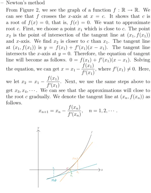
– Newton’s method
From Figure 2, we see the graph of a function f : R → R. We can see that f crosses the x-axis at x = c. It shows that c is a root of f (x) = 0, that is, f (c) = 0. We want to approximate root c. First, we choose a point x1 which is close to c. The point
x2 is the point of intersection of the tangent line at (x1, f (x1))
and x-axis. We find x2 is closer to c than x1. The tangent line
at (x1, f (x1)) is y = f (x1) + f0(x1)(x − x1). The tangent line
intersects the x-axis at y = 0. Therefore, the equation of tangent line will become as follows. 0 = f (x1) + f0(x1)(x − x1). Solving
the equation, we can get x = x1−
f (x1) f0(x1), where f 0(x 1) 6= 0. Here, we let x2 = x1 − f (x1) f0(x 1)
. Next, we use the same steps above to get x3, x4, · · · . We can see that the approximations will close to
the root c gradually. We denote the tangent line at (xn, f (xn)) as
follows. xn+1 = xn− f (xn) f0(xn), n = 1, 2, · · · . y x c 1 x 2 x 1 ( ) f x 2 ( ) f x f 3 x
Figure 2: Newton’s method
We consider the Newton’s method in Rn, n ≥ 2. We let function f : Rn → Rn. And we choose x which is a solution of f , that
is, f (x) = 0. By using the same steps above, we can obtain the formula as follows.
xn+1 = xn− f (xn) · Jf−1(xn), n = 1, 2, · · · ,
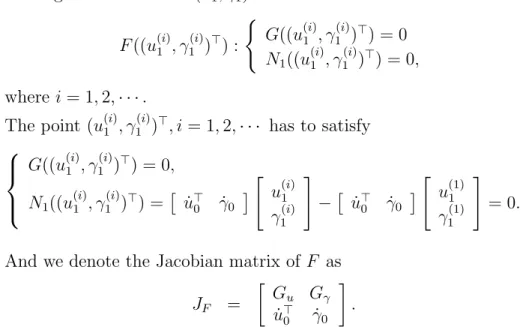
Now, we have the point (u(1)1 , γ1(1))>. We want to get the points which
converge to the solution (u1, γ1)>. We let
F ((u(i)1 , γ1(i))>) :
(
G((u(i)1 , γ1(i))>) = 0 N1((u(i)1 , γ
(i)
1 )>) = 0,
where i = 1, 2, · · · .
The point (u(i)1 , γ1(i))>, i = 1, 2, · · · has to satisfy
G((u(i)1 , γ1(i))>) = 0, N1((u(i)1 , γ1(i))>) =
£ ˙u> 0 ˙γ0 ¤" u(i) 1 γ1(i) # −£ ˙u> 0 ˙γ0 ¤" u(1) 1 γ1(1) # = 0. And we denote the Jacobian matrix of F as
JF = · Gu Gγ ˙u> 0 ˙γ0 ¸ .
Then, we use the formula of Newton’s method, that is, we solve the system as follows.
(u(i+1)1 , γ1(i+1))>= (u(i)1 , γ1(i))>− F ((u1(i), γ1(i))>) · JF−1((u(i)1 , γ(i)1 )>), where i = 1, 2, · · · .
Hence, we can get (u(2)1 , γ1(2))>, (u(3)
1 , γ
(3)
1 )>, · · · . We can find that (u (1)
1 , γ
(1) 1 )>
will converge to (u1, γ1)>. Repeating the method, we will get (u2, γ2)>, (u3, γ3)>, · · · .
0 0 (u,γ)Τ 1 1 ( ,u γ)Τ (1) (1) 1: 0( 1) 0( 1) 0 N u&Τu−u +γ& γ−γ = (1) (1) 1 1 (u ,γ )Τ 0 (0, 0) p=uΤγ Τ v & & 1 pv 2 N (1) (1) 2 2 (u ,γ )Τ 2 2 (u,γ)Τ
4.3
Quotient Transformation Invariant Continuation
Method
In this subsection, we will introduce the quotient transformation invariant continuation method [7]. And we replace standard continuation method with the quotient transformation invariant continuation method. In the process of computing, some problems will occur. We need to overcome these problems. First, we will face the problem about the predicting directions. Before discussing the problem, we consider the solution curve of standard continu-ation method. From equcontinu-ation (4.4), we know that there are four variables and three equations. Consequently, we can get the solution which is a two-dimensional manifold. We denote the solution set of equation (4.4) as M. Hence, we suppose that the solution will be a pipeline.
M
Figure 4: standard continuation method
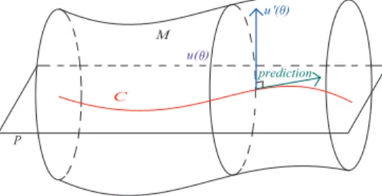
From Figure 4, we can see that why the standard continuation method will fail. We will find that the predicting directions will move along the manifold. As a result, we can not get meaningful predictions of standard continuation method. Hence, we want to use quotient transformation in-variant continuation method which can improve the disadvantage. For the purpose of letting the solution of equation (4.4) can be a straight line, we add a plane to equation (4.4). Thus, there are four variables and four equations.
M C '( ) u prediction P ( ) u θ θ
From Figure 5, we can see that the direction of predictions will be on the plane. And the quotient solution curve C is on the plane P . We will explain the details of the process of transformation.
From equation (4.5), we can rewrite into the forms as follows.
G(y(s)) = 0,
where y(s) = (u(s), γ(s)). And we differentiate G(y(s)) = 0 with respect to
s. Thus, we can get
JG(y(s)) ˙y(s) = 0, (4.8)
where JG(y(s)) is the Jacobian matrix of G. And we denote a tangent vector
of C at y(s) as ˙y(s) = ( ˙u(s)>, ˙γ(s))>. We let C be the quotient solution curve.
We show that the conception of quotient solution. Let
u(θ) = u · eiθ,
= (u1+ iu2) · eiθ,
= u1cos θ + iu1sin θ + iu2cos θ − u2sin θ,
= (u1cos θ − u2sin θ) + i(u1sin θ + u2cos θ).
We define u(θ) = · u1cos θ − u2sin θ u1sin θ + u2cos θ ¸ .
Let equation (2.3) be multiplied in both right and left sides by eiθ. We
can obtain the equation as follows.
[−∆u + iγ∂θ1u + V u + α1|u|
2u] · eiθ = λ
1u · eiθ.
We know that u will satisfy equation (2.3) if u is a solution. And we suppose that u · eiθ will be a solution, that is,
[−∆ + iγ∂θ1 + V + α1|u · e
iθ|2]u · eiθ = λ
1u · eiθ. (4.9)
We put |u · eiθ|2 = |u|2|eiθ|2 = |u|2 into equation (4.9). Then, we can get
[−∆ + iγ∂θ1 + V + α1|u| 2]u · eiθ = λ 1u · eiθ, ⇒[−∆ + iγ∂θ1 + V + α1|u| 2]u = λ 1u.
And we consider the normalized constraint. Z
|u · eiθ|2dx =
Z
Hence, we can verify the assumption, that is, if u is a solution, then ueiθ
is also a solution. We can see that the solution M contains transformation invariant solutions u(θ).
We denote the quotient solution as C. Now, we want to get the tangent vector of u(θ). Hence, we will differentiate u(θ) with respect to θ. We can get
u0(θ) =
·
−u1sin θ − u2cos θ
u1cos θ − u2sin θ
¸
. (4.10)
We choose θ = 0 and put it into equation (4.10). Then we can get u0(0) = ∂u ∂θ(0). ∂u ∂θ(0) = · −u2 u1 ¸ = (−u> 2, u>1)>.
Consequently, we can obtain the normal vector of the plane which we add, that is, the tangent vector of u(θ). We denote (∂u
∂θ(0)>, 0)> as the tangent
vector.
Then, we begin the further exploration of the quotient transformation invariant continuation method. First, we discuss the part of prediction. We know that the prediction vector ˙y(s) = ( ˙u(s)>, ˙γ(s))>. And ( ˙u(s)>)> is
perpendicular to the tangent vector (∂u
∂θ(0)>, 0)>. Next, we consider the part
of correction. We can see that the vector of correction will be on the plane which we add. And the normal vector of the plane is (∂u
∂θ(0)>, 0, 0)>.
• predictions
By using fixed point iteration method, we can get the initial solution
(u0, γ0)> ∈ R(2N +2)×1. We let y0 = (u0, γ0)>. We discuss how we find
the vectors of predictions. In the part of predictions, we know that the vector of predictions will be on the plane P . The plane has the normal vector (∂u
∂θ(0)>, 0, 0)>. The vector of predictions ˙y(s) = ( ˙u(s)>, ˙γ(s))>
should satisfy the equation (4.8). And ( ˙u(s)>)> is perpendicular to the
tangent vector (∂u
∂θ(0)>, 0)>. Therefore, we add a plane as follows. a>θ ˙u = 0, (4.11) where aθ = ( ∂u ∂θ(0) >, 0)> = (((−u>2, u>1)>)>, 0)> = (−u> 2, u>1, 0)>.
Originally, we solve the system of (4.7). We let y(s) = (u(s), γ(s)) and ˙y(s) = ( ˙u(s)>, ˙γ(s))>. Hence, we can rewrite it into the form as
follows. £
Gu Gγ ¤ ˙y(s) = 0.
Since we add a plane which is satisfied equation (4.11), we have to solve the system as follows.
· Gu Gγ a> θ 0 ¸ ˙y = · 0 0 ¸ .
By computing above, we can get the vectors of predictions. Conse-quently, we will get the new solution (u(1)1 , γ1(1))> = (u
0, γ0)>+ ¯s · ˙y,
where k ˙yk2 = 1.
In the process of predictions, we let yi = (ui, γi)> be the approximate
solution every time. And we have to solve the system as follows. · Gu Gγ a> θ 0 ¸ ˙yi = · 0 0 ¸ . (4.12)
Then, we denote the vector of prediction as ˙yi = ( ˙u>i , ˙γi)>. As a result,
we will get the new solution (u(1)i , γi(1))>= (u
i−1, γi−1)>+ ¯si· ˙yi, where i = 1, 2, · · · , ¯si is the length of step every time and the two norm of ˙yiis
equivalent to one. After computing the vector of predictions, we hope that the new solution will converge to the solution by using Newton’s method. Hence, we introduce the steps of corrections.
• corrections
We continue discussing the correction part of quotient transforma-tion invariant continuatransforma-tion method. Now, we have the new solutransforma-tion (u(1)i , γi(1))> which is on the plane P
i. Here, Pi represents the plane
which has the normal vector (∂u
∂θ(0)>, 0)>. And we know that the
vec-tor of corrections will also be on the plane Pi. The solutions which will
proceed to converge are also on the plane. We want to get the vectors of correction. As a result, we have to consider the system as follows.
G : G(u, γ) = 0, P : a> θ ˙u = 0,
Ni : ˙u>i−1u + ˙γi−1γ = ˙u>i−1u
(1)
i + ˙γi−1γi(1)
It means that the solution curve is related to the system above. We know that the point which we want to find has to satisfy the system,
that is, (ui, γi)>. We consider the system as follows. H = G : G(ui, γi) = 0, P : a> θ ˙ui−1= 0,
Ni : ˙u>i−1ui+ ˙γi−1γi = ˙u>i−1u
(1)
i + ˙γi−1γi(1)
For the purpose of getting the vectors of corrections, we still use New-ton’s method. Therefore, we consider the Jacobian matrix of H, that is, JH = Ga>u Gγ θ 0 ˙u> i−1 ˙γi−1 ∈ R(2N +3)×(2N +2). (4.13)
Then, we use Newton’s method to solve it iteratively. And we put it into the formula as follows.
(ui(n+1), γi(n+1)) = (u(n)i , γi(n)) − H(u(n)i , γi(n)) · J−1 H (u (n) i , γ (n) i ),
where n = 1, 2, · · · . Hence, we can get the solutions which will converge gradually. We stop the steps of correction until the solutions converge.
• improvement in computing
Now, we have the system H and JH. In the process of computing, we
observe the last row of Gu. We will find that the norm of the last row
is much smaller than other rows. It will result in error in calculation. The last row will be ignored. To review the system H which we want to solve, we observe G3, that is, the normalized constraint. We let
G3 be multiplied in both sides by accuracy. And we let accuracy =
max(k(u, γ)k, 1). We also let the planes P and Ni be multiplied in both
sides by accuracy. Now, we have new normalized constraint, in other words, we rewrite G3 to accuracy · (C>U0 − 1). And we rewrite the
planes into the forms as following.
P : accuracy · (a>θ ˙ui−1) = 0,
Ni : accuracy · ( ˙u>i−1ui+ ˙γi−1γi) = accuracy · ( ˙u>i−1u
(1)
i + ˙γi−1γi(1)).
By using the skill above, we can obtain H and JH accurately. And we
have to rewrite equation (4.5) as follows.
Gu = ¯ A + α1(3u°12 + u° 2 2 ) 2α1(u1◦ u2) − γS −u1 2α1(u1 ◦ u2) + γS A + α¯ 1(3u°22 + u° 2 1 ) −u2 accuracy · (2C>◦ u> 1) accuracy · (2C>◦ u>2) 0 ∈ R(2N +1)×(2N +1).
In the part of prediction, system (4.12) has to rewrite into the form as follows. · Gu Gγ accuracy · a> θ 0 ¸ ˙yi = · 0 0 ¸ .
Furthermore, we consider the part of prediction. We rewrite equation (4.13) into the form as follows.
JH =
accuracy · aGu > Gγ
θ 0
accuracy · ˙u>
i−1 accuracy · ˙γi−1
∈ R(2N +3)×(2N +2).
4.4
Algorithm
In this section, we will introduce the algorithm of continuation method. We can see that the algorithm consists of predictions and corrections. We show the Algorithm as follows.
Step1. Computing initial value Compute initial value: (u0, γ0).
Set the length of step.
Set count = the number of possible solutions. Step2. Predictions for i = 0, 1, · · · ,count Compute JacobF = · Gu(ui, γi) Gγ(ui, γi) accuracy · a> θ 0 ¸ .
Find the desired singular values and singular vectors of JacobF.
Let the smallest singular vector be the vector of predictions: P red uγ. end
Step3.
(u(1)i+1, γi+1(1)) = (ui, γi)+step·P red uγ.
If step< 10−8, stop. Compute JH; Here, G = · G P ¸ ; H = · G N ¸ .
Step4. Corrections (Newton’s method) Compute Del uγ = −JH−1· H(u(1)i+1, γi+1(1))
(u(2)i+1, γi+1(2)) = (u(1)i+1, γi+1(1)) + Del uγ. ComputeJH, N, G, H
and kDel uγk > 10−7)
step = step/2 and go to Step3 else
go to Step5 end
Step5. Corrections (Newton’s method) for j = 2, 3, · · · ,
If (kH(u(j)i+1, γi+1(j))k > 10−8· accuracy) Del uγ = −J−1 H · H(u (j) i+1, γ (j) i+1)
(uj+1i+1, γi+1j+1) = (uji+1, γi+1j ) + Del uγ. ComputeJH, N, G, H
if(kH(u(j)i+1, γi+1(j))k/kH(u(j+1)i+1 , γi+1(j+1))k < 5) if(kDel uγk < 10−7)
stop else
step = step/2 and go to Step 2. end
end else
(u(j)i+1, γi+1(j)) → (ui+1, γi+1) and go to Step6.
end end
Step6. Save
Compute accuracy=pkJHkk(ui+1, γi+1)k
if accuracy < 1 accuracy=1 end
Go to Step 2.
5
Numerical Results
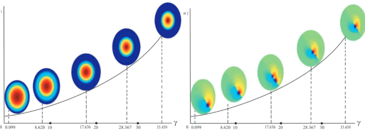
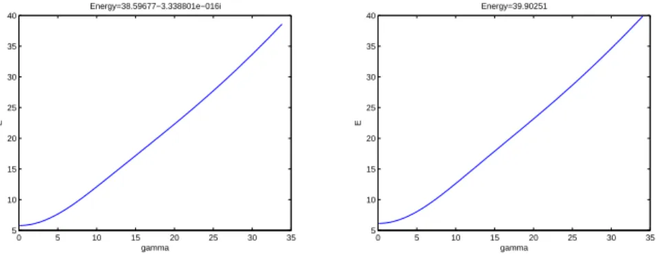
We use quotient transformation invariant continuation method to approxi-mate the solution curve. In this section, we will show that the numerical results as follows. First, we can see that the approximative solution curve in Figure 6 and Figure 7. In Figure 6 and Figure 7, γ represents the value of x-axis. And the values of y-axis are pu2
1+ u22,u1,u2 separately. Next, to
change the value α1, we observe the changes of energy. From Figure 8 and
we let α1 = 0, 1, 5, 10. Finally, we show that the difference between the
eigenvalue λ1 and the energy functional E(φ) is α21
R
|u|4. We compute the
difference, that is, λ1 − E(φ) − α21
R
|u|4. And we obtain the value is 10−7
approximately. Hence we can verify that the relation between the eigenvalue and the energy functional.
γ
0 0.099 8.62010 17.63620 28.367 30 35.459
2 2 1 2
u+u
Figure 6: Case: α1 = 5, N = 50 × 50, the value of y-axis:
p u2 1+ u22. γ 00.099 8.62010 17.63620 28.367 30 35.459 1 u γ 00.099 8.62010 17.63620 28.367 30 35.459 2 u
Figure 7: Case: α1 = 5, N = 50 × 50, the value of y-axis: left graph:u1, right
0 5 10 15 20 25 30 35 5 10 15 20 25 30 35 40 Energy=38.59677−3.338801e−016i gamma E 0 5 10 15 20 25 30 35 5 10 15 20 25 30 35 40 Energy=39.90251 gamma E
Figure 8: left graph: α1 = 0, right graph: α1 = 1
0 5 10 15 20 25 30 35 40 5 10 15 20 25 30 35 40 45 50 Energy=45.55085+2.779894e−016i gamma E 0 5 10 15 20 25 30 35 40 5 10 15 20 25 30 35 40 45 50 55 Energy=52.70174−2.740863e−016i gamma E
Figure 9: left graph: α1 = 5, right graph: α1 = 10
6
Conclusions
We discuss the process of discretization on a nonlinear Schr¨odinger equation and introduce the standard continuation method. In the process, we face on the difficult computing problem. Hence, we improve the method by using the quotient invariant transformation continuation method. In order to find the solution curve successfully, we add the plane. Hence, we can see the diagrams of approximate solution curve in section 5. We also verify the relation between the eigenvalue and the energy functional.
References
[1] Chia-Feng Tsao. Numerical study of a two-component Bose-Einstein
condensate in magnetic field. preprint, 2007.
[2] Volodymyr Sushch On some discrete model of the magnetic Laplacian. preprint, 2002.
[3] I.Schindler, K.Tintarev A nonlinear Schr¨odinger equation with external
magnetic field. preprint.
[4] Ambar K. Mitra Finite Difference Method for the Solution of Laplace
Equation. preprint.
[5] H.B. Keller. Lectures on Numerical Methods In Bifurcation problems. Springer-Verlag, 1987.
[6] Yuen-Cheng Kuo, Wen-Wei Lin, Shih-Feng Shieh, Weichung Wang. A
Hyperplane-Constrained ContinuationMethod for Bound States of Cou-pled Nonlinear Schr¨odinger Equations. (Submitted), 2007.
[7] Yuen-Cheng Kuo , Wen-Wei Lin , Shih-Feng Shieh, and Weichung Wang.
Exploring Bistability in Rotating Bose-Einstein Condensates by a Quo-tient Transformation Invariant Continuation Method. (Submitted)
[8] Shu-Ming Chang, Yuen-Cheng Kuo, Wen-Wei Lin, Shih-Feng Shieh.
A Continuation BSOR-Lanczos-Galerkin Method for Positive Bound States of A Multi-Component Bose-Einstein Condensate . J. Comput.
Phys., 210(2):439-458, 2005.
[9] W. Z. Bao. Ground states and dynamics of multi-component
Bose-Einstein condensates. SIAM Multiscale Modeling and Simulation, 2(2):210-236,2004.