An efficient probabilistic dynamic multicast routing in ATM networks

Received May 20, 1997; accepted May 27, 1998. Communicated by Jean-Lien C. Wu.

485

An Efficient Probabilistic Dynamic Multicast Routing

In ATM Networks

KUOCHEN WANGAND JUN-HUNG CHEN Department of Computer and Information Science

National Chiao Tung University Hsinchu, Taiwan 300, R.O.C. E-mail: kwang@cis.nctu.edu.tw

In this paper, we propose a dynamic multicast routing algorithm based on

probabil-ity for multimedia communications in an asynchronous transfer mode (ATM) network

environment. For multimedia communications, we not only aim to arrange a transmission path with the minimal cost from a source node to each destination node, but also consider the dynamic multicast situation with node joining/leaving. To meet the above requirements, we develop a new method based on the relative probability of each node being truncated from the multicast connection tree, such that we can arrange a better path for a new joining node in such a way as to reduce the impact of leaving requests caused by other nodes in the multicast connection tree. The main contribution of this paper is a new and efficient dy-namic multicast routing algorithm for multimedia communications which keeps the whole multicast connection tree near optimal in terms of cost inefficiency and guarantees that the transmission delay will be less than the preset bounded end-to-end delay. Simulation re-sults show that under various sizes of networks and requests, the cost inefficiency of the multicast connection tree constructed by our approach is less than those of the trees con-structed by the greedy algorithm and the weighted greedy algorithm, respectively.

Keywords: dynamic multicast routing, probability, minimal spanning tree, bounded delay,

ATM network, multimedia communication, greedy algorithm

1. INTRODUCTION

In recent years, the asynchronous transfer mode (ATM), which can support large bandwidth and is connection-oriented, has been developed to support broadband integrated service digital networks (B-ISDN). ATM networks will be an important part of the network technology used to achieve multimedia communications, especially in video and audio applications. To solve the bottleneck in the bandwidth available for multimedia communications, we should not only increase the available bandwidth, but also reduce the number of superfluous cells in transmission links. Multicast communications, which deliv-ers the same messages from a source node to an arbitrary number of destination nodes simultaneously, will be an important technology in the future. The multicast routing prob-lem is that of constructing a minimal cost connection tree from a source node to all destina-tion nodes [1-5]. In general, solving a multicast routing problem involves tree construcdestina-tion. There are two reasons for basing efficient multicast routes on trees [6]: (1) the data can be transmitted in parallel to various destination nodes along the branches of the tree; (2) a minimum number of copies of data is transmitted, with duplication of data being necessary

only at forks in the tree. There are two styles of multicast routing: one is one-to-many transmission and the other is many-to-many transmission [7, 8]. In the first case, distance learning is a popular application while video conferencing is a practical application of the other [9]. In this paper, we focus on the one-to-many model which is a multicast connec-tion tree with one source node and multiple destinaconnec-tion nodes. For many-to-many transmission, we can apply one-to-many transmission when a node wants to transmit data to other nodes, so one-to-many transmission can be extended to many-to-many transmission. Two different optimization goals can be used in multicast routing algorithms to deter-mine what constitutes a good tree [10]. One such goal is providing the minimum delay along the tree, which is important for distributed real-time computing environments. An-other optimization goal is allocating network resources as efficiently as possible for multi-media communications, which usually involves a heavy load. For applications in multime-dia communications, one important characteristic is that the multicast group (destination nodes) may be dynamic. That is, some destination nodes may leave the multicast connec-tion tree, and other external nodes may also join the tree. Some algorithms have been proposed to solve the dynamic multicast routing problem. These algorithms are of two types: path rearrangeable, where a connection path can be modified during the transmis-sion period [12-15], and path unrearrangeable, where a connection path can not be changed [16-18]. Connection-oriented networks, such as ATM networks, suit use of the path unrearrangeable algorithm due to the heavy cost of reordering the cell sequence. Some algorithms for arranging dynamic multicast connection paths, which are suitable for con-nection-oriented networks, are described as follows.

The greedy algorithm [16] arranges the shortest link in order to add a new node to the multicast connection tree. It is a simple method for path unrearrangeable networks. The greedy algorithm has the minimum cost for node joining requests, but node leaving re-quests will lead to extra cost compared with the cost of the optimal multicast connection tree. The study by Subranmanian and Liu [5] showed that the greedy algorithm results in a solution which is worse than the optimal case after some join/leave operations because it can not handle the unpredictable node leaving request. Huang and Tanaka [17] used a predictive method to improve the drawback of the greedy algorithm. It arranges a route for a new joining node based on the traffic load of nodes in the multicast connection tree. The algorithm must work on the premise that we can predict the traffic load of the whole network. This is difficult in most cases. Waxman [18] proposed a weighted greedy algorithm (WGA) to reduce the impact of node leaving requests so that the greedy algorithm can be improved. The fundamental idea of WGA is that a new joining node should not be too far from the source node, so that the cost of the whole multicast connection tree will not be heavily affected when some nodes in the multicast connection tree submit leaving requests. However, WGA has better performance than the greedy algorithm only in small networks with fewer than 20 nodes. In our proposed algorithm, we try to keep the advantages of the above algorithms. Our algorithm searches for a minimum cost connection path for a new joining node and minimizes the impact of node leaving requests by calculating the relative trun-cated probability of each node in the multicast connection tree. In this paper, we will first define the multicast routing problem for multimedia communications and present a dy-namic multicast routing algorithm to construct a near-optimal spanning tree from a source node to all destination nodes. We guarantee that the maximum delay of each transmission

path is less than the preset bounded end-to-end delay. Our proposed algorithm can meet the characteristics of ATM networks because it is connection-oriented, it guarantees quality of service (QOS), and it keeps the cell order [11].

This paper is organized as follows. Section 2 gives an overview and survey of exist-ing multicast routexist-ing algorithms that include static multicast routexist-ing and dynamic multicast routing. Section 3 defines the network model. Section 4 presents our probabilistic dy-namic multicast algorithm along with complexity analysis. In section 5, we analyze the simulation results and make comparisons with those obtained using the greedy and WGA algorithms. We discuss the simulation results and some implementation issues in section 6. Finally, some conclusion remarks are made in section 7.

2. MULTICAST ROUTING PROBLEM

In general, there are two types of multicast routing:

∑ Static multicast routing: the destination nodes do not change during the

transmis-sion period.

∑ Dynamic multicast routing: the destination nodes can leave the multicast

connec-tion tree or other nodes could join the tree during the transmission period. We will give an overview of the multicast routing problems and survey some existing static and dynamic multicast routing algorithms in the following subsections.

2.1 Static Multicast Routing

The feature of static multicast routing is that the source and the destination nodes are predefined before the multicast connection tree is constructed. The main task of the static multicast problem is to construct a minimal cost connection tree covering the source and all preset destination nodes [18-20]. Since the multicast routing problem can be solved by means of tree construction, the cost optimization problem can be based on graph theory. We can reduce the static multicast routing problem to the minimum Steiner tree problem (MST) [21]. Formally, the MST in graphs can be stated as follows [18]. Given

∑ a graph G = (V, E), with node set V and edge set E, ∑ a cost function, Cost: E Æ R+_{, and}

∑ a subset of vertices S Õ V,

find a subtree T = (VT, ET) of G which spans S, which will be the multicast connection tree, such that the Cost (T) = SeΠE_T Cost(e) is minimized. The MST has been proven to be an

NP-complete problem [22]. Previous works on heuristic solutions to the MST problem can be classified into two approaches [18]. The first approach, that of constructing a minimum spanning tree by connecting likely intermediate nodes to the source and all destination nodes, was proposed by Rayward-Smith [23]. The other approach, that of first construct-ing a minimum spannconstruct-ing tree coverconstruct-ing all the nodes in the whole graph, removconstruct-ing

superflu-ous nodes and then trying to include more intermediate nodes which can reduce the overall cost of the spanning tree, was proposed by Kou,Markowsky and Berman [24], and is re-ferred as the KMB algorithm.

2.2 Dynamic Multicast Routing

In contrast to static multicast routing, dynamic multicast routing allows destination nodes to join or leave the multicast connection tree during the transmission period. Unlike static multicast routing, the main problem in dynamic multicast routing is that the cost of the multicast connection tree will no longer be optimal after some nodes join or leave the tree. There are three possible ways to solve the problem [25]:

1. re-route the whole tree whenever one node leaves or joins the multicast connection tree;

2. initially construct an optimal tree and make minimal to changes; 3. choose a suboptimal tree that will be resilient to change.

The first and second ways are suitable for the path rearrangeable mode, and the last one is suitable for the path unrearrangeable mode. Since an ATM network must guarantee the cell sequence, changing the connection path during the transmission period will result in a large overhead required to maintain the cell order. Most of the algorithms [6, 17, 25] assume that the existing transmission paths will not be modified in the ATM network environment. Generally, the dynamic multicast algorithm considers two operations: re-moving a node from the connection tree (the deletion operation) and joining a new node in the connection tree (the addition operation). In the deletion operation, since the transmis-sion path can not be modified, the algoritm just checks if the node that wants to leave the multicast connection tree is a leaf node or not. If it is not a leaf node, this means that the node still needs to relay ATM cells to other nodes; then it is marked as a non-destination (intermediate) node. Otherwise, the node is deleted from the multicast connection tree. This procedure is recursively applied to the node’s parent until the node is no longer a leaf node.

As to node addition, this is an NP-complete problem of arranging a new path for a new node. We will introduce two heuristic algorithms, the greedy algorithm [16] and the WGA [18]. In section 5, we will compare our probabilistic heuristic algorithm with these two algorithms because the greedy algorithm is the most instinctive method and the WGA is specially designed for the dynamic multicast problem in unrearrangeable networks. Al-though the greedy algorithm is easy to implement, its performance will be worse than the optimal case after some addition (+) and deletion (-) operations. For example, as shown in

Fig. 1, we can see that after three addition and two deletion operations, the cost (19 units) of the final graph (shown in Fig. 1(f ) ) will be worse than that (16 units) of the optimal graph (shown in Fig. 1(g)) though the original graph is optimal in the initial state (when nodes A, C, E are added). Note that the optimal graph is an optimal multicast connection tree which is defined as a minimum spanning tree recalculated after new joining/leaving requests are completed [6]. Waxman proposes the WGA to improve the greedy algorithm [18]. In WGA, the source node s is chosen as the owner of the multicast connection tree, with a constraint that node s must remain in the connection tree. For the node addition operation in WGA, the new adding node u is connected to the node v, already in the tree, which minimizes the function [18]

W(v) = (1 - w) . d(u, v) + w . d(v, s) 0 £ w £ 0.5,

where d(x, y) is the cost from x to y. We can find that if w = 0, then WGA is equivalent to the greedy algorithm. When w = 0.5, WGA chooses the shortest path from u to s. In this algorithm, the value of w can be adjusted so as to increase or decrease the relative signifi-cance between the adding path d(u, v) and the existing path d(v, s). Fig. 2 illustrates WGA with the same add/delete sequence shown in Fig. 1. When node D submits a joining request (shown in Fig. 2(d)), the WGA chooses link (D, E) to connect node D to the connection tree (shown in Fig. 2(e)) instead of adding links (D, F) and (F, G). This is done to keep node D from being far from the source s and to minimize the influence of node G leaving. In this respect, WGA improves the drawback of the greedy algorithm. This reduces the total cost of the whole tree from 19 to 17 units. One problem with WGA is setting the value of w. Inspecting the above function, we can find that different values of w will produce different results, and that different network topologies will need different values of w. Although Waxman asserts that w = 0.3 will lead to better results [18], we have found that the perfor-mance of WGA will be worse than that of the greedy algorithm in a large network accord-ing to our simulation results given in section 5.

Fig. 1. A dynamic multicast routing example: [+(A, C, E), +G, -E, +D, -G], using the greedy algo-rithm and the corresponding optimal graph.

9 8 3 1 1 9 8 3 1 1 9 8 3 1 1 9 8 3 1 1 9 8 3 1 1 9 8 3 1 1 9 8 3 1 1 A 3 D F C _E 4 3 4 7 G B ₃ A D F C _E 4 3 4 7 G B A 3 D F C _E 4 3 4 7 G B A ₃ D F C _E 4 3 4 7 G B A 3 D F C _E 4 3 4 7 G B A 3 D F C _E 4 3 4 7 G B (f) final graph (e) delete G A 3 D F C 4 3 4 7 B G E (g) optimal graph Source node Destination node Non-used link Transmission link Non-used node Intermediate node

(a) add (A,C,E) (b) add G (c) delete E (d) add D

s s s s s s s

3. NETWORK MODEL

The network topology is modeled as a weighted graph G = (V, E) with node set V and edge set E. The nodes in V are of three types [10]:

∑ source node: the node used to send a data stream to other nodes and denoted as s; ∑ destination node set: the set of nodes which receives the data stream from the source

node, denoted as S;

∑ intermediate node set: the set of those nodes which are intermediate hops in a path

from the source node to a destination node.

For each edge e ΠE, we define two weight functions, C(e) and D(e). C(e) is a cost function

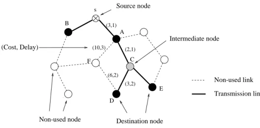
on edge e, and D(e) is a delay function on edge e. The delay in an ATM network consists of a queueing delay, transmission delay and propagation delay. We assume that the delay function D(e) is proportional to the length of edge e. The cost function C(e) is associated with the bandwidth utilization of edge e. The higher the utilization is, the higher the cost is. An example of this network model is shown in Fig. 3. The node s is the source node, S = { A, B, D, E} is the destination node set, and node C is an intermediate node. For the weight functions of an edge, (3, 1) in edge (s, A) denotes that 3 cost units and 1 time unit will be required for transmission of a cell from s to A. The heavy-lines denote the multicast con-nection tree from the source node s to the destination node set S.

Fig. 2. A dynamic multicast routing example: [+(A, C, E), +G, -E, +D, -G], using WGA and the corresponding optimal graph (w = 0.3).

9 8 3 1 1 9 8 3 1 1 9 8 3 1 1 9 8 3 1 1 9 8 3 1 1 9 8 3 1 1 9 8 3 1 1 A 3 D F C _E 4 3 4 7 G B ₃ A D F C _E 4 3 4 7 G B A 3 D F C _E 4 3 4 7 G B A ₃ D F C _E 4 3 4 7 G B A 3 D F C _E 4 3 4 7 G B A 3 D F C _E 4 3 4 7 G B (f) final graph (e) delete G A 3 D F C 4 3 4 7 B G E (g) optimal graph Source node Destination node Non-used link Transmission link Non-used node Intermediate node

(a) add (A,C,E) (b) add G (c) delete E (d) add D

s s

s s s

A network topology is constructed by distributing n nodes at random [18]. All nodes are permitted to exist at any location with integer coordinates. For each pair of nodes, a distance in (0, L] is chosen based on a random distribution, in which L is the maximum possible distance between two nodes. An edge is introduced between a pair of nodes u and v, with a probability that depends on the distance between them. The edge existence probability, which was proposed by Waxman [18], is

P u v d u v L e( , ) exp ( , ) , =β − _α

where d(u, v) is the distance from u to v, and a and b are parameters in the range (0,1]. Larger values of b result in graphs with higher edge densities while smaller values of a increase the density of shorter edges relative to longer ones. Each graph is generated at random and must be tested to ensure that it is a connected graph. That is, a spanning tree exists which covers all the nodes in the network topology.

4. DESIGN APPROACH

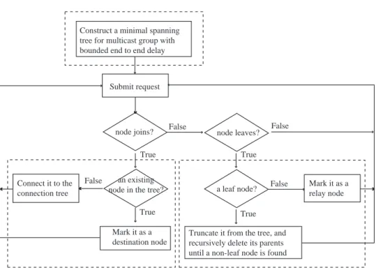
The flowchart of the proposed algorithm is shown in Fig. 4. It can be divided into three parts, which are enclosed by dashed-lines. The first part is construction of a multicast connection tree which covers the source node and all initial destination nodes using a static multicast routing algorithm; the second part deals with the situation in which a destination node in the tree submits a leaving request, and the last part shows what happens when a node submits a joining request. These three parts are explained in the following.

Fig. 3. The network model. Source node Intermediate node F A (3,1) E (2,1) B D Destination node (6,2) (3,2) (10,3) s C (Cost, Delay) Non-used node Non-used link Transmission link

Fig. 4. Flowchart of probabilistic dynamic multicast routing.

4.1 Initial Connection Setup

In the initial stage, a multicast connection tree is established between the source and all destination nodes. The problem of finding a minimal cost spanning tree can be trans-formed into the Steiner tree problem. The KMB algorithm [24] is a near-optimal algorithm for solving the Steiner tree problem. We first compute the minimal cost paths for all pairs of nodes using the shortest path algorithm in graph theory, which is similar to the KMB algorithm. By choosing the minimal paths from the source to all destination nodes, we can repeatedly construct a connection path from the source to a destination node until all the destination nodes are included in the multicast connection tree. Note that the total delay from the source to each destination node must be less than the preset bounded delay. After ths is done, we have constructed an initial multicast connection tree. Now, we will discuss the situations of node leaving and node addition (joining). We define a request list as a list of nodes which have made requests to leave or join the multicast connection tree.

4.2 Node Leaving

When one destination node submits a leaving request, we just check whether it is a leaf node in the multicast connection tree. If it is not a leaf node, it is marked as an interme-diate node. Otherwise, the node is truncated from the multicast connection tree, and its parent is recursively truncated until a non-leaf node, a destination node, or the source node

Construct a minimal spanning tree for multicast group with bounded end to end delay

Submit request

node joins? node leaves?

a leaf node? an existing

node in the tree? False False False False True True True True Mark it as a relay node

Truncate it from the tree, and recursively delete its parents until a non-leaf node is found Connect it to the

connection tree

Mark it as a destination node

is reached. Because the multicast connection tree has been modified, it may be not an optimal connection tree. In the case of a packet switched network, we can adjust the con-nection tree to obtain the minimal cost spanning tree because it is a concon-nectionless network. But in the ATM network environment, we must guarantee the cell sequence. If we change the connection paths during the transmission period, cells may get out of sequence. This will result in large overhead required to recover the cell order. With the limitation that the path cannot be rearranged, the improvable space available for node leaving is finite. Consequently, arranging a better connection path for a new destination node is an improv-able part of dynamic multicast routing.

4.3 Node Addition

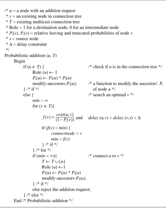
The node addition part of our probabilistic dynamic multicast routing algorithm is shown in Fig. 5. Assume that each destination node has a relative leaving probability (Pl) such that it will submit a leaving request and a relative truncated probability (Pt) that it will be truncated from the multicast connection tree. Note that only the relative values of these probabilities are important. The derivation of these two parameters will be described later. An intermediate node in the multicast connection tree also has a relative truncated probabil-ity (Pt) of being truncated from the tree. It depends on the relative truncated probabilities of its children. If a destination node is a leaf node in the tree, then Pt = Pl. It will be truncated from the multicast connection tree when it submits a leaving request. If a node in the multicast connection tree is not a leaf node, then its Pt depends on its Pl and the Pt’s of its children in the multicast connection tree. For example, node C (an intermediate node) in Fig. 3 will be truncated from the multicast connection tree when destination nodes D and E both submit leaving requests. Note that Pl(C) = 1. Therefore, the relative truncated prob-ability of node C, Pt(C), will be the relative truncated probprob-ability of node D, Pt(D), times the relative truncated probability of node E, Pt(E). Similarly, truncating node A in Fig. 3 from the multicast connection tree not only depends on the relative leaving probability of node A, but also on the relative truncated probability of node C. That is, the relative trun-cated probability of node A, Pt(A), will be Pl(A) . Pt(C) = Pl(A) . Pt(D) . Pt(E).

We use the following equation to define Pt(v), the relative truncated probability of node v:

P v_t( )=P v_l( )⋅∏P i_t( ), node which is a child of node ∀ i, v.

Based on the previous deduction, we can find a new connection path such that the impact of leaving requests made by other nodes can be minimized when a new node wants to join the multicast connection tree. The main idea is to choose an existing node with a small connec-tion cost to be the new node and to keep the relative truncated probability of the existing node as small as possible. We propose the following cost function to choose a node v if node u wants to join the multicast connection tree:

f v u v

P vt delay s u

( ) ( , )

( ( )) ( , ) ,

= −cost₁ <∆

where v is a node in the connection tree that is to be connected to node u; cost(x, y) is the cost in terms of bandwidth utilization or delay from node x to node y; D is the preset bounded

delay(s, u) is the delay from the source node s to the new addition node u, which is delay(s, v) + delay(v, u). The value of this function can be derived for each node v in the multicast connection tree, and the node with the minimal value is selected. Assume this node is v; the connection path from node u to node v will have the minimal value f(v). We show an example to illustrate our algorithm in Fig. 6. Note that this is the same example used to illustrate the greedy (shown in Fig. 1) and the WGA (shown in Fig. 2), respectively. When

Fig. 5. Node addition in our probabilistic dynamic multicast routing.

/* u = a node with an addition request * v = an existing node in connection tree * T = existing multicast connection tree

* Role = 1 for a destination node, 0 for an intermediate node * Pl(v), Pt(v) = relative leaving and truncated probabilities of node v * s = source node

* D = delay constraint

*/

Probabilistic-addition (u, T) Begin

if (u Œ T) { /* check if u is in the connection tree */ Role (u) ¨ 1

Pt(u) ¨ Pt(u) * Pl(u)

modify-ancestors-Pt(u); /* a function to modify the ancestors’ Pt

} /* if */ of node u */

else { /* search an optimal v */

min = • for (v Œ T){ f v u v P vt ( ) ( , ) ( ( ))

= −cost1 and delay (u,v) + delay (v,s) < D if (f(v) < min) { connectnode = v min = f(v) } /* if */ } /* for */ if (min < •){ /* connect u to v */ T ¨ T »{u} Role (u) ¨1

Pt(u) ¨ Pt(u) * Pl(u) modify-ancestors-Pt(u); } /* if */

else reject the addition request; } /* else */

node D submits a joining request as shown in Fig. 6(d), our probabilistic algorithm chooses node A to connect with node D because f(A) is the minimum for all the neighbors {A, C, E, G} of node D. Fig. 6(e) shows the final graph, which is identical to the optimal graph shown in Fig. 6(f).

4.4 Complexity Analysis

To analyze the complexity of our algorithm, we divide the algorithm into three parts, as shown in Fig. 4. In the first part, it takes O(|V|3_{) to construct a multicast connection tree} for the initial multicast group, where |V | is the number of nodes in the network. For the second part of node leaving, it takes O(H(T)) (not greater than |V |), where H(T) is the height of the multicast connection tree T. It marks a leaving node as an intermediate node or truncates the node and some of its ancestors. For the last part of node addition, it takes O(|T |) (not greater than |V |) to choose the best connection link from the new joining node to the multicast connection tree, where |T | is the number of nodes in the multicast connection tree. Thus, the complexity of our algorithm is O(|V |3 _{+ H(T)+|T |) = O(|V |}3_{). Comparing it with} the greedy and WGA algorithms, our algorithm has the same complexity as the other two although it needs to modify the relative truncated probability Pt of the multicast connection tree when a node leaves or joins the multicast group. The complexity of modifying Pt is O (H(T)) because only the relative truncated probabilities of the leaving/joining node and its ancestors in the multicast connection tree are modified.

Fig. 6. A dynamic multicast routing example: [+(A, C, E), +G, -E, +D, -G], using the proposed algorithm and the corresponding optimal graph (Pl = 0.3).

(9,3) (8,2) (3,1) (1,1) (1,2) (9,3) (8,2) (3,1) (1,1) (1,2) (9,3) (8,2) (3,1) (1,1) (1,2) (9,3) (8,2) (3,1) (1,1) (1,2) (9,3) (8,2) (3,1) (1,1) (1,2) (9,3) (8,2) (3,1) (1,1) (1,2) (9,3) (8,2) (3,1) (1,1) (1,2) A D F C _E G B A D F C _E G B A D F C _E G B A D F C _E G B A D F C _E G B A D F C _E G B (f) final graph (e) delete G A D F C B G E (g) optimal graph Source node Destination node Non-used link Transmission link Non-used node Intermediate node (a) add (A,C,E) (b) add G (c) delete E (d) add D

(3,1) (7,3) (4,2) _(3,1) (4,1) (3,1) (7,3) (4,2) _(3,1) (4,1) (3,1) (7,3) (4,2) _(3,1) (4,1) (3,1) (7,3) (4,2) _(3,1) (4,1) (3,1) (7,3) (4,2) _(3,1) (4,1) (3,1) (7,3) (4,2) _(3,1) (4,1) (3,1) (7,3) (4,2) _(3,1) (4,1) s s s s s s s

5. SIMULATION RESULTS

In this section, we will analyze the simulation results obtained using our probabilistic algorithm, the greedy algorithm and the WGA. Finding a minimum cost path is the most important and critical requirement in multimedia communications because of the possibil-ity of heavy loads in transmission links. These algorithms can be compared using the cost inefficiency dH, which is defined as follows [6]:

δH H O O C C C = − ,

where CH is the cost of a multicast connection tree using a heuristic algorithm, and CO is the cost of the optimal multicast connection tree, which is a minimum spanning tree recalcu-lated after joining/leaving requests are completed [6]. For a large network, finding the optimal multicast connection tree is impractical. We redefine the cost inefficiency (dH¢ ) with respect to a near-optimal multicast connection tree as follows [6]:

′ = − ′ ′ δH H O O C C C ,

where C_O′ is the cost of a near-optimal multicast connection tree constructed by using a static multicast routing algorithm. In order to show the validity of our algorithm in every circumstance, all network topologies and request lists were generated at random. The net-work size was from 5 to 100 nodes, and the cost of each edge was from 1 to 100, which is a function of the bandwidth utilization or delay of a selected channel. Note that the delay of an edge is proportional to the edge length.

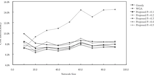
The following simulation results are for average cases. We first simulated the case with a fixed Pl for each destination node. Later, we simulated the case with a random Pl for each destination node. Fig. 7 shows the relationship between cost inefficiency and network size with Pl = 0.1 to 0.5 for these three algorithms. The simulation results show that the performance (cost inefficiency) of our scheme is better than that of the other two schemes when the relative leaving probability is less than 0.5. Even when the relative leaving prob-ability is 0.5, our algorithm performs better than WGA and also performs better than the greedy algorithm in most situations. These results prove that the performance of our algo-rithm is very stable with respect to wide variations of the relative leaving probability for each node. The performance of WGA is much worse than that of the other two schemes for a large network. The main difference between WGA and our algorithm is that WGA con-siders adding a new node to an existing node which has a lower connection cost (or is closer) to the source node, while our algorithm considers adding a new node to an existing node with a lower relative truncated probability, which is related to the relative truncated probabilities of its children nodes. In this way, our scheme also indirectly considers adding a new node to an existing node which has a lower connection cost to the source node. Such an existing node also has a lower truncated probability since it is closer to the source node. As to the greedy algorithm, it is suitable for join-only dynamic multicast tree construction. The reason why the greedy algorithm performs better than WGA for a large network is that the merit of adding a new node to an existing node which has a lower connection cost to the source node may be offset by the merit of using a lower cost edge between the new node and the existing node. Note that in the paper on WGA [18], only a small network of less than 20 nodes was evaluated.

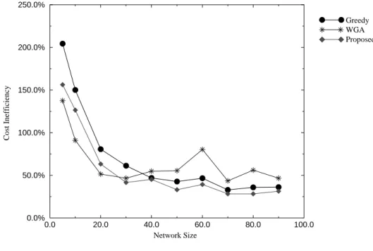
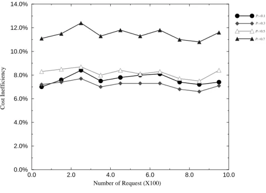
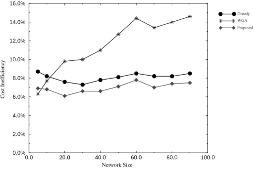
In Fig. 8, we show the cost inefficiencies of the three algorithms with respect to different numbers of requests, which range from 1 to 1000. Our algorithm also performs better than the other two algorithms when the number of requests is greater than 100. To sum up, in most cases, the cost inefficiency of the multicast connection trees constructed using our algorithm is less than that of trees constructed using the other two algorithms, under different network sizes and numbers of requests. In Fig. 9, we show the worst case cost inefficiency of each of these three algorithms. The worst case cost inefficiency of our algorithm is still less than that of either of the other two algorithms for most network sizes. Fig. 10 shows the cost inefficiency of our algorithm under different network sizes and relative leaving probabilities. Fig. 11 shows the cost inefficiency of our algorithm under different numbers of requests and relative leaving probability. Based on these two figures, the relative leaving probability of a node should be between 0.1and 0.5 in practical applications. The simulation results show that Pl in the neighborhood of 0.3 yields the best result. Pl = 0.1 yields higher cost than 0.3 because the former is close to 0. In this situation, the algorithm will be close to the greedy algorithm, which does not consider the relative leaving probability of a node. In addition, Pl = 0.7 yields the worst cost because it predicts that the nodes in the network will leave the multicast connection tree very quickly, which does not match the characteristic of multimedia communications. Up to now, we have discussed the situation where each destination node has the same relative leaving probability. In real applications, we can assign different relative leaving probabilities to various nodes based on the attributes of their local subscribers, such as their age, sex, character, job, etc., in the joining requests. For example, an earnest student will have a lower leaving probabil-ity than a student who is frequently absent in a distance learning system. By assigning an appropriate relative leaving probability to each destination node, our probabilistic algo-rithm can arrange a better connection path for a node addition operation. As shown in Figs. 12 and 13, we assign a random relative leaving probability to each destination node. The simulation results again show that our algorithm has the minimal cost inefficiency among the three dynamic multicast algorithms for most cases.

Fig. 7. Cost inefficiency versus network size.

4.0% 6.0% 8.0% 10.0% 12.0% 14.0% 16.0% 0.0 20.0 40.0 60.0 80.0 100.0 Cost Inefficiency Greedy WGA Proposed Pl =0.1 Proposed Pl =0.2 Proposed Pl =0.3 Proposed Pl =0.4 Proposed Pl =0.5 Network Size

Fig. 8. Cost inefficiency versus number of requests with Pl = 0.3.

Fig. 9. Worst case cost inefficiency versus network size with Pl = 0.3.

0.0 2.0 4.0 6.0 8.0 10.0 Number of Requests (X100) 0.0% 2.0% 4.0% 6.0% 8.0% 10.0% 12.0% 14.0% 16.0% Cost Inefficiency Proposed Greedy WGA 0.0 20.0 40.0 60.0 80.0 100.0 Network Size 0.0% 50.0% 100.0% 150.0% 200.0% 250.0% Cost Inefficiency Greedy WGA Proposed

Fig. 10. Cost inefficiency versus network size with various Pl.

Fig. 11. Cost inefficiency versus number of requests with various Pl.

0.0 2.0 4.0 6.0 8.0 10.0 Number of Request (X100) 0.0% 2.0% 4.0% 6.0% 8.0% 10.0% 12.0% 14.0% Cost Inefficiency Pl =0.1 Pl =0.3 Pl =0.5 Pl =0.7 0.0 2.0 4.0 6.0 8.0 10.0 Number of Request (X100) 0.0% 2.0% 4.0% 6.0% 8.0% 10.0% 12.0% 14.0% Cost Inefficiency Pl =0.1 Pl =0.3 Pl =0.5 Pl =0.7

Fig. 12. Cost inefficiency versus network size with random Pl in each destination node.

Fig. 13. Cost inefficiency versus number of requests with random Pl in each destination node.

0.0 20.0 40.0 60.0 80.0 100.0 Network Size 0.0% 2.0% 4.0% 6.0% 8.0% 10.0% 12.0% 14.0% 16.0% Cost Inefficiency Greedy WGA Proposed 0.0 2.0 4.0 6.0 8.0 10.0 Number of Requests (X100) 0.0% 2.0% 4.0% 6.0% 8.0% 10.0% 12.0% 14.0% 16.0% Cost Inefficiency Greedy WGA Proposed

Our proposed algorithm can also be made fault tolerant to node and edge failures. Since the cost of each edge may denote the bandwidth utilization or delay of a selected channel, the cost of an edge can be set to be infinite if an edge fails. The algorithm will not choose a faulty edge, so it can tolerate the edge failure. In the case of a node failure, the costs of all edges connected to the node can be set to be infinite. By updating the cost of each edge periodically, our algorithm can still work well under both node and edge failures.

6. DISCUSSION

In this section, we will discuss the simulation results and some implementation issues related to the proposed, the greedy and the WGA algorithms. Our algorithm can reduce the cost inefficiency of WGA by as much as 50%. Although the improvement of our algorithm over the greedy algorithm is not more than 2%, as shown in Figs. 8, 12, and 13, the band-width savings or delay reduction obtained using our algorithm for large networks may be still very considerable. Our approach trades a small connection setup time overhead for a low bandwidth requirement of bandwidth-demanding (in several Mbps) multimedia appli-cations or for a low delay of real-time multimedia appliappli-cations. Compared with the cost of the multicast connection tree, the connection setup time (routing time) may not be a crucial parameter in dynamic multicast routing for multimedia communication applications be-cause the connection time (in hours) is usually much longer than the connection setup time (in seconds). Note that the complexity of our algorithm, which is related to the connection setup time, is the same as that of the other two algorithms, as shown in section 4.4. Al-though the margin of improvement may be offset by uncertainty in parameter measurement and stochastic variation, in the worst case, our algorithm still performs better than the other two algorithms no matter a fixed preferred relative leaving probability (shown in Figs. 7 and 8) or a random relative leaving probability (shown in Figs. 12 and 13) is used for each node. These results prove that the performance improvement of our algorithm over the other two algorithms is very stable with respect to wide variation of the relative leaving probability for each node.

We can apply the proposed algorithm to dynamic multicast applications, such as video on demand and distance learning. The relative leaving probability of a node can be derived by multiplying the product of the leaving probabilities of its local subscribers by an adjust-ing constant that can be determined through experimentation. As long as the relative leav-ing probability of each node is available, the relative truncated probability of each node can be derived easily. At the beginning of the deployment of our scheme in a multimedia application (e.g., video on demand) in an ATM network, since we do not have the leaving probabilities of local subscribers in each node, we may use a fixed preferred relative leav-ing probability of 0.3 for each node, as shown in Figs. 7 and 10. As the network collects more information about each node from the past history of submitted leaving requests, we can derive a more appropriate relative leaving probability by relating the leaving probabili-ties of local subscribers to their age, sex, character, job, selected video program, etc.

In a wide area ATM network environment [26], the network can be viewed as a hierarchical network. As an example, in a two-level network, the network consists of sev-eral regional subnetworks. First, we multicast a multimedia application from the main source node to each regional selected source node. Then, each regional subnetwork can

run our multicast routing algorithm. In this way, our algorithm can match the distributed nature of the network. As to the quality of service (QOS), if we consider the cost of an edge as a function of its delay (or distance) instead of as a function of bandwidth utilization, then cost inefficiency can address a little bit of QOS. However, to have a guaranteed QOS, such as bounded end-to-end delay, all three algorithms need another constraint in order to re-strict the overall delay between the source node and each destination node, as shown by our cost function in section 4.3.

7. CONCLUSIONS

Dynamic multicast routing will in the future be a basic requirement for multimedia communications in an ATM network environment. To guarantee the cell sequence in ATM networks, a multicast routing model with unrearrangeable connection paths during the trans-mission period is used. This is also considered to prevent large overhead due to cell reordering. Another important problem for dynamic multicast routing is keeping the multicast connection tree optimal after several join/leave operations. A node addition scheme is the key to the path unrearrangeable multicast routing model. In this paper, we have presented a novel probabilistic dynamic multicast routing algorithm to construct a delay-bounded multicast connection tree with low cost inefficiency for ATM networks. We use the relative truncated probability to locate a better node position so as to activate an edge for node addition, where the purpose is to keep the impact of node leaving operations on the total cost as small as possible. Simulation results show that our algorithm performs better than the greedy or weighted greedy algorithms, respectively, under various network sizes, num-bers of requests, and a wide range of relative leaving probabilities. The cost inefficiency of our probabilistic algorithm is up to 50% less than that of the weighted greedy algorithm. In practical applications, our probabilistic algorithm can assign a relative leaving probability for each destination node more precisely through experimentation so as to arrange a better connection edge for a new addition node. As a result, the reduction in cost inefficiency obtained using our algorithm will be even better than that obtained using either of the other two algorithms. Some implementation issues have also been addressed to demonstrate the feasibility of our approach.

REFERENCES

1. C. Huang, C. C. Huang and P. K. McKinley, “Communication issues in parallel com-puting across ATM networks,” IEEE Parallel and Distributed Technology: Systems and Applications, Vol. 2, No. 4, 1994, pp. 73-86.

2. J. M. S. Doar, “Multicast routing in the asynchronous transfer mode environment,” Computer Laboratory Technical Report, University of Cambridge, 1993.

3. M. H. Ammar, S. Y. Cheung and C. M. Scoglio, “Routing multipoint connections using virtual paths in an ATM network,” in Proceedings of IEEE INFOCOM ’93, Vol. 1, 1993, pp. 95-105.

4. C. A. Noronha Jr. and F. A. Tobag, “Optimum routing of multicast streams,” in Pro-ceedings of IEEE INFOCOM ’94, Vol. 2, 1994, pp. 865-873.

5. N. Subramanian and S. Liu, “Centralized multi-point routing in wide area networks,” in Proceedings of the 1991 Symposium on Applied Computing, 1991, pp. 46-52. 6. V. P. Kompella, J. C. Pasquale and G. C. Polyzos, “Multicast routing for multimedia

communication,” IEEE/ACM Transactions on Networking, Vol. 1, No. 3, 1993, pp. 286-292.

7. X. Jia, “A total ordering multicast protocol using propagation trees,” IEEE Transac-tions on Parallel and Distributed Systems, Vol. 6, No. 6, 1995, pp. 617-627.

8. M. Grossglauser and K. Ramakrishnan, “SEAM: scalable and efficient ATM multicast, ” in Proceedings of IEEE INFOCOM ’97, 1997, pp. 868-876.

9. M. H. Willebeek-LeMair, D. D. Kandlurm and Z. -Y. Shae, “On multipoint control units for videoconferencing,” in Proceedings of 19th Conference on Local Computer Networks, 1994, pp. 356-364.

10. Q. Zhu, M. Parsa and J. J. Garcia-Luna-Aceves, “A source-based algorithm for delay-constrained minimum-cost multicasting,” in Proceedings of IEEE INFOCOM ’95, Vol 1, 1995, pp. 337-385.

11. R. Handel, M. N. Huber and S. Schroder, ATM Networks: Concepts, Protocols, Applications, Addison-Wesley, 1994.

12. H. Tode, Y. Sakai, M. Yamamoto, H. Okada and Y. Tezuka, “Multicast routing algo-rithm for nodal load balancing,” in Proceedings of IEEE INFOCOM ’92, Vol. 3, 1992, pp. 2086-2095.

13. A. G. Waters and T. L. J. Bishop, “Delay considerations in multicast routing for ATM networks,” Tenth UK Teletraffic Symposium Performance Engineering in Telecommu-nications Networks, 1993, pp. 12/1-6.

14. J. Kadirire and G. Knight, “Comparison of dynamic multicast routing algorithms for wide-area packet switched (asynchronous transfer mode) networks,” in Proceedings of IEEE INFOCOM ’95, Vol. 1, 1995, pp. 212-219.

15. F. Bauer and A. Varma, “ARIES: a rearrangeable inexpensive edge-based on-line steiner algorithm,” in Proceedings of IEEE INFOCOM ’96, Vol. 1, 1996, pp. 361-368. 16. G. Brassard and P. Bratley, Algorithms: Theory and Practice, Prentice-Hall, 1988, pp.

79-104.

17. P. C. Huang and Y. Tanaka, “Multicast routing based on predicted traffic statistics,” IEICE Transactions on Communications, Vol. E77-B, No. 10, 1994, pp. 1188-1193. 18. B. M. Waxman, “Routing of multipoint connections,” IEEE Journal on Selected Areas

in Communications, Vol. 6, No. 9, 1988, pp. 1617-1622.

19. C. H. Chow, “On multicast path finding algorithms,” in Proceedings of IEEE INFOCOM ’91, Vol. 3, 1991, pp. 1274-1283.

20. B. K. Kadaba and J. M. Jaffe, “Routing to multiple destinations in computer networks,” IEEE Transactions on Communications, Vol. COM-31, No. 3, 1983, pp. 343-351. 21. F. K. Hwang and D. S. Richards, “Steiner tree problems,” Networks, Vol. 22, No. 1,

1992, pp. 55-89.

22. R. E. Miller and J. W. Thatcher, “Reducibility among combinatorial problems,” in R. M. Karp (ed.), Complexity of Computer Computations, New York: Plenum, 1972, pp. 85-103.

23. V. J. Rayward-Smith and A. Clare, “On finding Steiner vertices,” Networks, Vol. 16, No. 3, 1986, pp. 283-294.

24. L. Kou, G. Markowsky and L. Berman, “A fast algorithm for Steiner trees,” Acta Informatica, Vol. 15, 1980, pp. 141-145.

25. M. Doar and I. Leslie, “How bad is naive multicast routing,” in Proceedings of IEEE INFOCOM ’93, Vol. 1, 1993, pp. 82-89.

26. J. Kadirire and G. Knight, “Exploiting geographic spread (GS) for wide-area asyn-chronous transfer mode (ATM) dynamic multipoint routing,” Fifth IEE Conference on Telecommunications, 1995, pp. 262-267.

Kuochen Wang (¤ý°êºÕ ) received the B.S. degree in con-trol engineering from National Chiao Tung University, Taiwan, in 1978, and the M.S. and Ph.D. degrees in electrical engineering from the University of Arizona in 1986 and 1991, respectively. He is currently an associate professor in the Department of Com-puter and Information Science, National Chiao Tung University. From 1980 to 1984, he worked on network management and on the design and implementation of the Toll Trunk Information Sys-tem at the Directorate General of Telecommunications in Taiwan. He served in the army as a second lieutenant communication pla-toon leader from 1978 to 1980. His research interests include computer networks, mobile computing and wireless networks, fault-tolerant computing, and computer-aided VLSI design.

Jun-Hung Chen (³¯«T§» ) received the B.S. and M.S. de-grees in computer and information science from National Chiao Tung University, Taiwan, in 1991 and 1996, respectively. His re-search interests include ATM networks, network management, cli-ent server computing, and fault-tolerant computing.