國
立
交
通
大
學
ၥଉऋᏰᇄώแंـܚ!
ቺ
!
ҳ
!
ᑕ
!
Ԏ
!
無線感測網路中使用空間和時間編碼之資
料壓縮技術
Data Compression in Sensor Networks
with Spatial and Temporal Coding Techniques
研 究 生:謝燿宇
無線感測網路中使用空間和時間編碼之資料壓縮技術
Data Compression in Sensor Networks
with Spatial and Temporal Coding Techniques
研 究 生:謝燿宇 Student:Yao-Yu Hsieh
指導教授:曾煜棋 Advisor:Yu-Chee Tseng
國 立 交 通 大 學
資 訊 科 學 與 工 程 研 究 所
碩 士 論 文
A ThesisSubmitted to Institute of Computer Science and Engineering College of Computer Science
National Chiao Tung University in partial Fulfillment of the Requirements
for the Degree of Master
in
Computer Science
June 2007
無線感測網路中使用空間和時間編碼之資料壓縮技術
學生:謝燿宇 指導教授:曾煜棋 國立交通大學資訊科學與工程研究所 摘要 無線通訊和嵌入式微感測器技術顯著的進步使得結合這兩種技術的無網線 感測網路成為可能。環境觀測,用於收集並分析位於遠端環境的感測器回傳的數 值,便成為一種無線感測網路中具有商業發展潛力的應用。在環境觀測的應用 中,減少無線感測網路中節點能源的消耗對於系統壽命以及系統穩定度是非常重 要的。在這篇論文中,我們提出了利用資料在時間和空間上有相似性的資料壓縮 演算法來減少無線感測網路中的資料傳輸,進而延長無線感測網路的系統壽命。 此外,我們實作了利用上述的資料壓縮演算法的資料收集及查詢平台,並且此平 台上作了相關實驗來檢測它的效能。實驗的結果表示我們的系統可以在維持高度 的資料正確性之前提下有效地減少資料傳輸。 關鍵字: 資料相似性,訊息壓縮,普及運算,感測器資料管理,無線感測網 路。Data Compression in Sensor Network
with Spatial and Temporal Coding Techniques
Student: Yao-Yu Hsieh Advisor: Yu-Chee Tseng
Department of Computer Science National Chiao-Tung University
Abstract
The remarkable advances of wireless communication and embedded micro-sensing MEMS technologies have made wireless sensor networks possible. Environment monitoring - the collection and analysis of sensor readings to observe remote region - is an important application of networked embedded sensing with significant commercial potential. In monitoring applications, reducing energy consumption is crucial to the life time and system reliability of wireless sensor networks. In this paper, we propose data compression algorithms exploiting spatial and temporal data correlation to reduce the amount of transmission and then prolong the system life time of wireless sensor networks. Besides, we also implemented a query and monitoring system based on these data compression algorithms and do some experiments to test its performance. The results show our system can save energy efficient while maintains data accuracy at the same time.
Keyword: data correlation, message compression, pervasive computing, sensor data
誌 謝
首先我要感謝我的指導老師曾煜棋教授在這兩年內的照顧和指導,曾教授除 了指引我,給予我目標和方向外,也給我很多的空間讓我能自由發揮和想像。從 他身上,我學到了許多研究的方法,對於他的感謝實在是筆墨難以形容。另外, 也要感謝王友群學長的指導和幫助,他時常對我的研究給予寶貴的意見,並且在 我遇到折挫時適時地拉我一把,同時他也對這篇論文貢獻良多,沒有他就沒有這 篇論文這句話一點也不為過。也感謝高速通訊與計算實驗室的學長同學們,給了 我很多指導和建議,他們的鼓勵是我在壓力大時能繼續走下去進而完成這篇論文 的動力。最後,要感謝我的父母和家人,感謝他們的養育之恩,並且提供我衣食 無虞的環境,讓我能夠無後顧之憂地投入研究,完成這篇有微薄貢獻的論文。謹 以這篇論文獻給我的父母,以及所有指導過我,幫助過我的人。Contents
中文摘要 Abstract 誌謝 Contents List of Figures Chapter 1 IntroductionChapter 2 Related Work
Chapter 3 Architecture
3.1 Spatial Compression Algorithm
3.2 Temporal Compression Algorithm
3.3 Exponential Shrinking Storage (ESS) Algorithm
Chapter 4 Implementation Chapter 5 Simulation Chapter 6 Conclusion Biography i ii iii iv v 1 5 7 9 13 14 20 27 31 32
List of Figures
Figure 1.1: Indoor temperatures collected by four sensor nodes during a day. Figure 3.1: System architecture of the MRCQ framework (with three layers). Figure 3.2: An example of the RZS method, where the compression ratio γ = 0:9 Figure 3.3: The format of packet transmitted by a layer-3 processing node.
Figure 3.4: Concept of ESS
Figure 3.5: examples of ESS with timestamp = 6 and timestamp = 13 Figure 3.6: Redundant Storage and Solution
Figure 4.1: MoteBase architecture. Figure 4.2: Implementation Scenario. Figure 4.3: Experiment Results
Figure 4.4: Photo of implementation of MRCQ
Figure 4.5: User Interface of implementation of MRCQ
Figure 5.1: Data error rate under different degree of events (amp) Figure 5.2: Data error rate v.s. Flow amount
3 8 11 12 16 18 19 21 23 23 25 26 29 29
Chapter 1
Introduction
Wireless sensor networks (WSNs) provide a new opportunity for pervasive and context-aware monitoring of physical environments. Such a network is composed of numerous sensor nodes, each being a tiny wireless device that continuously collects information from its vicinity and reports to the remote sink through a multi-hop ad hoc manner [2]. A WSN is usually deployed in a region of interest to observe particular phenomena or track objects inside the region. Practical applications of WSNs include, for example, habitat monitoring, health care, smart home, and surveillance [22, 12, 19, 23].
Because sensor nodes are operated by small batteries and it is infeasible to recharge them or deploy new nodes in many scenarios, how to extend the network lifetime is a critical issue. In this paper, we consider WSNs that possess the following characteristics:
• These WSNs are deployed to provide long-term monitoring of some specified regions. In
this case, since sensor nodes continuously report what they sense to the sink, the commu-nication overhead will dominate their energy consumption. Moreover, sensor nodes close to the sink will suffer from heavy loads of message transmission, which leads to network congestion [6] and rapidly consumes their energy. As these nodes exhaust their energy,
the network will be destroyed. Thus, how to reduce the amount of message transmissions of sensor nodes plays a leading role in extending the network lifetime.
• Sensing data reported from sensor nodes often exhibit a certain degree of data correlation.
Specifically, the sensing readings of neighboring nodes may present highly spatial
corre-lation because they sense the same environment. These nodes may detect either the same
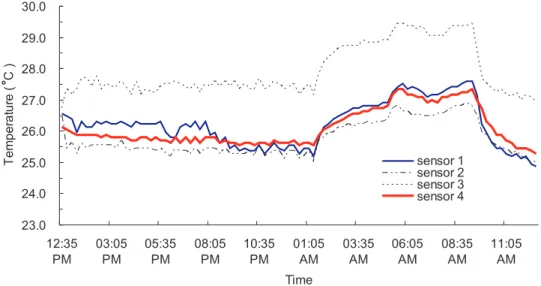
phenomenon or nothing from the environment. Besides, the sensing data collected by a single node may present highly temporal correlation when its surrounding environment remains stable. Fig. 1.1 illustrates an example, where we use four sensor nodes to collect the indoor temperatures during a day. From Fig. 1.1, we can observe that the temperatures reported by sensor nodes 1, 2, and 4 are quite similar (i.e., exhibit spatial correlation) be-cause they are close to each other, while the temperatures collected by an individual node during the time periods [12:35 PM, 05:35 PM] and [08:05 PM, 01:05 AM] remain stable (i.e., exhibit temporal correlation). With this observation, we can properly compress the sensing reports of nodes to reduce the amount of message transmissions.
• Users will query different “resolutions” of sensing data from the network [10, 8]. They
may periodically request a rough report from the sink to obtain an overview of the moni-toring environment. Occasionally, users could have interest to query detailed information from a subset of sensor nodes. With this requirement, sensor nodes should not only sim-ply report what they sense to the sink, but also have to maintain the sensing data in their local memories for further queries.
In this paper, we propose a multi-resolution compression and query (MRCQ) framework to provide message compression and multiple resolutions of sensing data in WSNs. The basic concept of our MRCQ framework is to organize the WSN into a hierarchical architecture and
23.0 24.0 25.0 26.0 27.0 28.0 29.0 30.0 12:35 PM 03:05 PM 05:35 PM 08:05 PM 10:35 PM 01:05 AM 03:35 AM 06:05 AM 08:35 AM 11:05 AM Time T e m p e ra tu re ( C ) sensor 1 sensor 2 sensor 3 sensor 4
Figure 1.1: Indoor temperatures collected by four sensor nodes during a day.
then establish multi-resolution summaries of sensing data by spatial and temporal compressions. These summaries of sensing data will be stored in the network for further query. Specifically, we organize the sensor nodes in a WSN into multiple layers. Messages transmitted by nodes in a lower layer will be compressed by a certain node in the upper layer through the spatial coding technology. Meanwhile, each node can also compress its sensing report by temporal coding method. In this way, the amount of message transmissions can be significantly reduced and thus the network lifetime can be prolonged. Moreover, in the MRCQ framework, nodes in each layer will keep a copy of their historical sensing data. Thus, users can query different resolutions and views of sensing data from different layers. In particular, they can obtain a coarser resolution but broader view of sensing data from a higher layer, and a narrower view but finer resolution from a lower layer.
Major contributions of this paper are three-fold:
• We develop a spatial and a temporal compression algorithms to help reduce the amount
but also the network congestion can be alleviated. In addition, our spatial compression algorithm allows users to set up different compression ratios. This can help users to bal-ance the tradeoff of data accuracy and energy consumption (due to message transmission) according to their application requirements.
• We design an efficient storage scheme to help sensor nodes to maintain a copy of their
historical sensing data in their local memories. This storage scheme considers the small size of sensors’ memories and attempts to record as much data as possible. This allows users to efficiently query long-term and finer data from sensor nodes.
• Our proposed compression and storage algorithms consider the limitation of computation
power and memory size of sensor nodes, so that they can be applied to practical sensor networks. To evaluate the performance and practicality of our MRCQ framework, we not only perform simulation studies but also implement a prototyping system on the MICAz MOTE platform [4].
The rest of this paper is organized as follows. Chapter 2 reviews some related works in the literature. Chapter 3 proposes the design of our MRCQ framework. Chapter 4 discusses the implementation of our prototyping system. Chapter 5 evaluates the system performance through simulations. Chapter 6 concludes this paper.
Chapter 2
Related Work
Data compression for textual content has been well studied in the literature. Huffman coding [17] and Lempel-Ziv-Welch (LZW) algorithm [21] are two popular text-coding compression schemes. They can provide lossless compression, in the sense that data can be completely recovered after decompression. However, the results of these text-coding compression schemes cannot be applied to the message compression in WSNs because the textual data are composed of a finite set of alphabets while the sensing readings in WSNs are usually continuous values. They cannot define the alphabets of sensing readings and thus fail.
On the other hand, wavelet transforms [24,20] are widely used in signal and image compres-sion. They attempt to preserve important features in a signal or an image while reduce those data that possess highly spatial and temporal correlation to the features to achieve data compression. For example, one well-known image compression algorithm, JPEG (joint photographic experts
group) [18], divides an image into multiple small square (called pixels), and then compress the
image by spatial correlation of these pixels. The concept of such wavelet compressions could be adopted to message compression in WSNs. However, these wavelet compression schemes usually suffer from high computation and space complexity. Thus, they may not be directly
applied to sensor nodes with very limited resources.
In-network data aggregation [13, 14, 16, 25, 7] also discusses how to reduce the amount of message transmissions by data similarity in WSNs. These methods attempt to “fuse” a set of similar sensing reports and generate one representative value to stand for these reports. For example, TAG [15] organize a sensor network into a tree structure and propose SQL-like se-mantics to construct streaming data aggregates such as histograms. Nevertheless, unlike data compression, this fusion operation is irreversible in the sense that the original sensing reports cannot be recovered. Thus, the subtle difference between sensing reports cannot be reflected since they have been fused together.
The work in [9] proposes a storage architecture called DIMENSIONS to support multi-resolution storage in a WSN. It organizes the network into multiple levels and adopts a wavelet compression scheme [5] in each level to generate spatiotemporal summarization of sensing data. Users then can obtain different resolutions of sensing reports from different levels via drill-down queries. However, as mentioned before, such a wavelet compression scheme requires a large cost of computation power and memory size. In DIMENSIONS, these high-cost wavelet compression and decompression operations are performed in each level, so that nodes in the network may suffer from higher computation and space complexity.
Chapter 3
Architecture
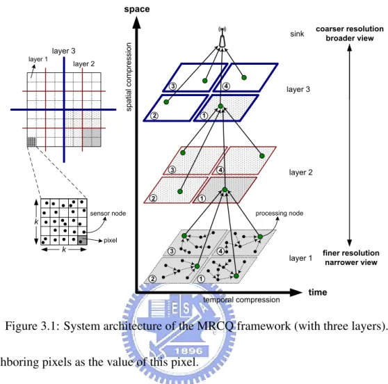
Fig. 3.1 illustrates the system architecture of our MRCQ framework. We assume that sensor nodes are homogeneous and are randomly deployed in the sensing field. In MRCQ, we recur-sively divide the network into quadruple blocks. In this way, the network will be organized into multiple layers, where a block in layer i + 1 contains four blocks in layer i. In each layer, we select a node in each block as the processing node [3, 11] to collect and compress sensing reports from the corresponding four blocks in the lower layer. The number of layers decides the resolutions and message sizes of sensing reports, and can be adjusted by users depending on their application requirements.
In layer 1 (i.e., the lowest layer), the processing node is responsible for compressing sensing reports from sensor nodes. In this layer, we further divide these nodes into k × k grids (called
pixels), where k is a small integer. Ideally, each pixel should contains exactly one node and we
use the sensing report of this node as the pixel’s value. Nevertheless, since sensor nodes are randomly deployed in the sensing field, it is possible that one pixel contains two or more nodes. In this case, we take the average of the sensing reports from these nodes as the pixel’s value. One the other hand, when a pixel contains no node, we will use the average of the values from
Figure 3.1: System architecture of the MRCQ framework (with three layers). the neighboring pixels as the value of this pixel.
In MRCQ, sensing data reported by sensor nodes are transmitted to the sink layer by layer. Messages passed through each layer will be compressed by the corresponding processing node in each block, through the spatial compression algorithm (discussed in Section 3.0.1). Sensor nodes and layer-1 processing nodes will also compress their data along the time axis by the
tem-poral compression algorithm (discussed in Section 3.0.2). To help users query past data from
the network, each node will storage the historical data in its local memory by the exponentially
shrinking storage (ESS) algorithm (discussed in Section 3.0.3).
Since the spatial and temporal compression algorithms will cause some loss of data preci-sion during the comprespreci-sion operation (depending on the comprespreci-sion ratio), processing nodes
in different layers will provide different resolutions of sensing data. In particular, users will obtain a coarser resolution (but broader view) by querying processing nodes in a higher layer. When they have interest in accessing more precious data, they can query the processing nodes in a lower layer. Note that each processing node stores and reports compressed data and these data are decompressed only at the sink. In this way, both the computation and space complexity of processing nodes can be greatly reduced.
3.0.1 Spatial Compression Algorithm
The spatial compression algorithm is performed by each processing node to compress sensing data from its lower layer. Users can specify a compression ratio γ (0 < γ ≤ 1) and this algorithm will compress these data based on their spatial correlation. According to the layer number, the spatial compression algorithm contains two parts: layer-1 compression and layer-i
compression (i > 1).
Layer-1 Compression
A layer-1 processing node collects the sensing data from its corresponding sensor nodes and
will store them in a k × k matrix M = (si,j)k×k. Then, we apply the 2D discrete cosine
transform (2D-DCT) [1] on M to generate a new matrix M0 = (t
i,j)k×k. In particular, for each
element ti,j ∈ M0, we have
ti,j = 2 kC(i)C(j) k−1 X x=0 k−1 X y=0 cos(2x + 1)iπ 2k cos (2y + 1)jπ 2k · si,j, (3.1) where C(i) = ½ 1 √ 2 if i = 1 1 otherwise .
The 2D-DCT is widely used in image processing. It can transform an image from spatial domain to the frequency domain and extracts significant values of the image. In particular, the
2D-DCT will compact those significant values in the upper-left part of the transformed matrix M0,
while leaving other insignificant values in the opposite part. In this way, we can still maintain most characteristics of the original matrix M by preserving only the upper-left part of the
transformed matrix M0and thus achieve message compression. However, the cosine operations
in Eq. (3.1) are too complicated for sensor nodes to calculate. Fortunately, the values of these cosine operations only depend on the system constant k (i.e., the length of matrix M). Thus, we can maintain a small table to keep the results of these cosine operations in each sensor node so that the complicated cosine calculation can be simplified as a table lookup operation.
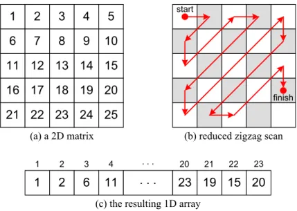
After calculating the matrix M0, we propose a reduced zigzag scan (RZS) method to
trans-late M0 into an 1D array D. In particular, the RZS method begins at the upper-left corner of
M0 and sequentially scan the diagonals of M0, as shown in Fig. 3.2. The RZS method stops
when it has scanned dk2· γe elements of M0. Then, we transmit the array D to the layer-2
pro-cessing node. With the property of 2D-DCT, the RZS method is guaranteed to maintain most significant values of the matrix M in the array D. Note that the compression ratio γ affects the data precision after decompressing D to the original matrix M (how to decompress will be discussed in Section 3.0.1). Specifically, we can maintain more information in the array D as γ becomes larger. Thus, the data precision can be increased after decompressing D.
Layer-i Compression
A layer-i (i > 1) processing node will further compress the data from its corresponding four blocks in the lower layer. Intuitively, one possible method is to first decompress the data from the lower layer and then apply the 2D-DCT method on these decompressed data to recompress
Figure 3.2: An example of the RZS method, where the compression ratio γ = 0.9. them again. Nevertheless, this method has two drawbacks. First, since the 2D-DCT method and its inversion are two expensive operations (for sensor nodes), the processing node will suffer from high computation complexity. The situation becomes worse in a higher layer because the processing node should handle a large amount of data from many sensor nodes. Second, this method may not help compress more data since in a large range of sensing field, the degree of spatial correlation of sensing data will degrade. Therefore, in layer-i compression, we simply
reduce the length of array D (passed from the layer i − 1) to dγi· k2e elements by discarding
the last bγi−1· k2− γi· k2c elements of D. Recall that the array D stores data in an decreasing
order by the data importance. Thus, we can compress the sensing data with the compression
ratio γiin layer i and still maintain the significant values of these data.
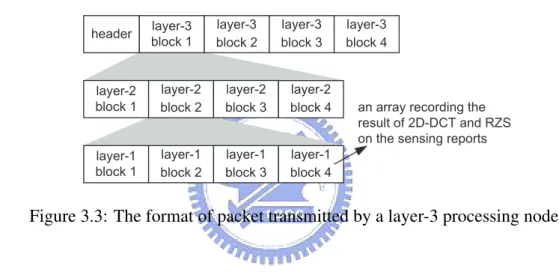
The processing node then combines these recompressed data of the corresponding four blocks in layer i − 1 in a clockwise sequence (i.e., following the sequences of the numbers marked in circles in Fig. 3.1). This makes the transmitted packet possess a structural form (as shown in Fig. 3.3) and thus can help the sink to recover the positions of blocks in each layer.
Next, we analyze the length of packets transmitted in each layer. Suppose that a sensor node takes l bits to transmit its sensing report and the length of a packet header is h. In layer 1, since the processing node maintains a k × k matrix to record the reports from sensor nodes,
the length of packet transmitted by a layer-1 processing node is thus h + dγ · k2le. For layer
2, the processing node further recompresses the data of its corresponding four layer-1 blocks,
so the length of packet transmitted by a layer-2 processing node is h + d(γ · k2l) × γ × 4e =
h + d4γ2· k2le. Similarly, the length of packet transmitted by a layer-i (i > 1) processing node
is h + d(4i−2γi−1· k2l) × γ × 4e = h + d4i−1γi· k2le.
header layer-3 block 1 layer-3 block 2 layer-3 block 3 layer-3 block 4 layer-2 block 1 layer-2 block 2 layer-2 block 3 layer-2 block 4 layer-1 block 1 layer-1 block 2 layer-1 block 3 layer-1 block 4
an array recording the result of 2D-DCT and RZS on the sensing reports
Figure 3.3: The format of packet transmitted by a layer-3 processing node.
Decompression Procedure
To reduce the computation overhead in each processing node, the decompression procedure is performed only at the sink. In particular, once the sink has collected the reports from the processing nodes in the highest layer, it first recovers the spatial locations of blocks in each layer according to the message received, as shown in Fig. 3.1. Then, for each layer-1 block, the sink translates the corresponding array D (which records the result of 2D-DCT and RZS on the
original sensing reports) into a 2D matrix M0 = (t
i,j)k×k by the RZS method. Since the array
D contains only d4d−1γd· k2e elements of compressed data, where d is the number of layers
M0. Finally, we adopt the inverse 2D-DCT to transform M0 to a new matrix M00 = (s
i,j)k×k.
In particular, for each element si,j ∈ M00, we have
si,j = 2 k k−1 X x=0 k−1 X y=0
C(x)C(y) cos(2i + 1)xπ
2k cos
(2j + 1)yπ
2k · tx,y.
Note that since the matrix M0 is incomplete, the transformed matrix M00 by the inverse
2D-DCT may not be necessarily equal to the original matrix M in Section 3.0.1 (i.e., lose some data precision). The compression ratio γ decides both the message size and data precision of sensing reports, which is a tradeoff between each other.
3.0.2 Temporal Compression Algorithm
The temporal data compression algorithms in data-collection tier and data-compression tier are similar. After the network is formed, the sink will broadcast the update threshold, δ to the whole network. The update threshold is used to design whether to update the value at higher level node or not. For a sensor node, once it sends its reading to its processing node, it will
record this reading to be the reference of comparison (vref). Next time before a sensor node
reports its reading, it compare the current reading (vcurrent) with (vref) first. Let d denotes the
difference between vcurrent and vref, then d = |vref − vcurrent|. If d < δ, which means the
difference between the current reading and the previous reported reading is not significant, then
the sensor node will not report vcurrent. Otherwise if d ≥ δ, this means the difference cannot be
neglected, then the sensor node will report this reading and replace its vref with vcurrent.
The temporal data compression algorithm of level-1 processing nodes is similar to that of sensor nodes. However, the reference of comparison is not a value but the whole matrix of
sensor readings. For a processing node at level 1, let Mref denotes the matrix of sensor readings
not report its current reading because of the spatial correlation, the processing node will not update the value of the sensor node, either. Before a spatial data compression is invoked, the processing node will verify whether the difference exceeds δ . The difference is denoted by:
d = 1 N2 N −1X i=0 N −1X j=0
|Mref[i, j] − Mcurrent[i, j]| (3.2)
If d < δ, the processing node will not send the result of applying spatial compression
algorithm on Mcurrent. Otherwise, if will send Mcurrent to its parent and replace the old Mref
with Mcurrent.
Unlike sensor nodes and processing nodes at level 1, processing nodes at higher levels do not keep a piece of reference data to decide whether to send current data. Since processing nodes will not decompress the data to retrieve the original reading, they are unable to estimate the difference between two sets of compressed data. Therefore, they only need to recompress received data with proper size and send these data to their parents. They do not apply any temporal compression algorithms.
3.0.3 Exponentially Shrinking Storage (ESS) Algorithm
In MRCQ, the compression rate of SDCM increases with level. Therefore, the sink, which is at the highest level of MRCQ, can only provide environment information with larger error and user can only be aware of the brief situation of the sensing field. Note that the precise sensing readings were not disappear; instead, they are scattered in the WSNs. Each processing nodes and sensing nodes keep a piece of data with higher accuracy, and users can query these nodes to retrieve data with higher accuracy. Therefore, storage mechanism are necessary for sensing
nodes and processing nodes. The storage mechanism must take the feature of limited-storage of devices in WSNs into consideration. Processing nodes and sensor nodes periodically store the current data with constraint space, and free space will definitely being exhausted. Therefore, some data must be discarded or merged to reduce the volume of used space to store more incoming data. This is a key feature of storage algorithm. In this subsection, we will introduce our exponential shrinking room storage algorithm (ESS), a storage algorithm to store past data of long time.
The concept of ESS is shown in Fig. 3.4. Each processing node and sensor node keeps a timer and a periodically incremented timestamp. Once the timer is fired, the timestamp is incremented and each processing node and sensor node stores the current data. We define a
frame as the data that a sensor node or processing node stores when the timer is fired and fi
as frame generated at timestamp i. The frame for a processing node is a single newly sensed sensing reading, while that of a processing node is the compressed data. Fig. 3.4 shows the data that a sensor node or a processing node stores at timestamp t. Suppose the memory space of a
node is capable of storing k frames, then a node will store ft, ft− 1, ft− 3, ft− 7, ... ft−2k−1+1.
When a node receives a query message regarding timestamp q, it first checks whether fq is in
the memory. If so, fq will be reported to the sink and the sink will show this sensing reading,
or decompress this frame; otherwise, this node will find two frames that q lies between these two timestamps and no other timestamp of available frames lies between this two timestamps, then send these two frames to sink. The sink will find the sensing reading or a set of data by interpolation.
Let the sequence of t, t − 1, t − 3, ... ,t − 2k−1+ 1 being the exponential sequence of
timestamp t. Ideally, the frames in the memory matches the exponential sequence of current timestamp. However, the memory space of devices in WSNs are limited, and it is impossible
Memory Space t t-1 t-3 t-7 Time Axis ft ft-1 ft-3 ft-7
Figure 3.4: Concept of ESS
for each node to store every frame of the past timestamp. When the memory space if full and a new frame requires a space, some frame will be discard. Unfortunately, this discarded frame will show in the exponential sequence of some timestamp but it no longer exists. Therefore, matching the exponential of each timestamp is impossible, but we can still try to approximate the exponential sequence by selecting the victim frame properly.
The detailed operation of ESS is described in this paragraph. Initially, all frames will be stored until the timestamp is larger than k, which means the space is not large enough to keep all frames, and some frame will be discarded. Actually, instead of discarding a frame, the ESS picks the k frames that approximate the current and following exponential sequences. Firstly, the oldest frame will be picked to guarantee that at least one frame with data describing situation long time ago exist. Therefore, this frame can be used as a reference of interpolation of query regarding data long time a ago. Note that frames of timestamp long time ago may gradually become insignificant. Therefore, if the difference between timestamp of the oldest frame and the current time stamp is larger than a pre-defined age, then the oldest frame is ”old enough to die” and loose the privilege of being the first picked frame. The privilege will be transferred to
the oldest and ”alive” frame.
After picking the oldest frame, ESS will pick k-1 frames with timestamps show in the cur-rent exponential sequence and future exponential sequence. The curcur-rent exponential sequence
is the first exponential sequence used as a target exponential sequence. For each timestamp si
in the target exponential sequence, ESS first finds a frame with timestamp as an agent which
equals to or has the least difference with si. Then ESS picks these agents in the order of the
differences. That is, agents equal to their siwill be picked first, and agents with large difference
to their siwill be picked after those with little difference have been picked. If ESS picks frames
for all si and the number of picked frame is less than k, then ESS selects the next exponential
sequence as the target exponential sequence and continues the frame picking procedure. Note that if an agent has already been picked, ESS will not pick this frame again to avoid keeping
redundant frames. If an si has two agent candidates, which means these tow agents have the
same difference with si, and one is larger than another, then ESS tends to pick the smaller one
as the agent. If the The frame procedure will be repeated until ESS picks k frames.
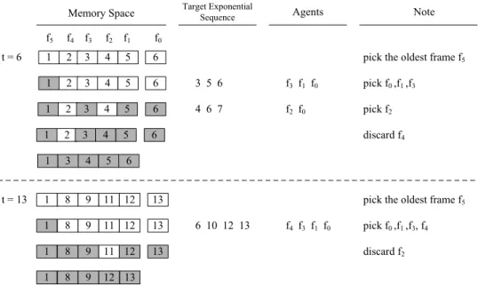
Fig. 3.5 shows examples of ESS frame picking procedure at timestamp 6 and timestamp 13
with k = 5. f5, f4 ... f1 represent the memory space, and f0 is the temporary storage. The
number in the rectangle is the timestamp of data that this frame stores. When the timestamp is 6, obviously the timestamps of stored data are 1 to 5 and there the temporary storage stores data generated at timestamp 6. Now ESS will discard one frame. The oldest while alive frame,
which is f5, is first picked. Then ESS find the current exponential sequence and their agents.
The agents of timestmap 3, 5 and 6 are f3, f1 and f0 respectively, whose timestamp are 3, 5
and 6. These three frames are not picked, so ESS picks these three frame. Then ESS find the
next exponential sequence, which is 4, 6 and 7. The agents of this exponential sequence are f2
1 2 3 4 5 f1 f2 f3 f4 f5 t = 6 6 Target Exponential Sequence Agents f0 6 1 3 4 5 6 1 2 3 4 5 3 5 6 Note 4 6 7 f2 f0 pick f2 f3 f1 f0 discard f4
1 2 3 4 5 6 pick the oldest frame f5
pick f0,f1,f3
t = 13 1 8 9 11 pick the oldest frame f5
6 10 12 13 f4 f3 f1 f0 pick f0,f1,f3, f4 12 13 1 8 9 11 12 13 1 8 9 11 12 13 discard f2 1 8 9 12 13 6 1 2 3 4 5 Memory Space
Figure 3.5: examples of ESS with timestamp = 6 and timestamp = 13
been picked, so ESS pick f2. After picking f2, ESS has picked 5 frames, which is the size of
memory, so the picking procedure ends, and the data of frame f4is discarded. Another example
shows the behavior of ESS at timestamp 13. The content of memory is shown if Fig. 3.5. As mentioned above, the oldest while alive frame is first picked. Then ESS find the agents of timestamps of the current exponential sequence. Frames with timestamp 6 and 10 are discard in past ESS, so the agent of 6 and 10 are frames with timestamp 8 and 9, which are closest to 6 and 10 respectively. The agents of timestmaps of the current exponential sequence are not picked, so ESS pick these frames and the number of picked frames are 5, then ESS terminate the frame-picking procedure at timestamp 13.
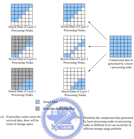
Each processing node store the compressed data received from lower layers. The recom-pression procedure is to discarding data at tail part of the compressed array generated by layer-1 processing nodes according to the compression rate and their layer. In this manner, the front part of compressed data are redundant because many processing nodes keeps the same piece
Stored Data of Layer 1 Processing Nodes Stored Data of Layer 2
Processing Nodes Stored Data of Layer 3
Processing Nodes
Stored but Redundant data Stored Data
If procedure nodes stores the received data, there will be waste of storage space (a)
Stored Data of Layer 3 Processing Nodes
Stored Data of Layer 2 Processing Nodes
Stored Data of Layer 1 Processing Nodes
Distribute the compressed data generated by layer processing nodes to processing nodes at different level can avoid the in-efficient storage usage probelm (b)
Compressed data at generated by a layer-1 processing node
Figure 3.6: Redundant Storage and Solution
of data, resulting in inefficient storage usage. Fig. 3.6(a) is an example of this problem. From Fig. 3.6, we can see that the stored data of processing nodes at layer i is the subset of that of processing nodes at layer i-1. Therefore, processing nodes at layer i-1 need not to store the data that processing nodes at layer i stores. They only need to store the data that processing nodes at layer i lacks. Fig. 3.6(b) shows the behavior.
Chapter 4
Implementation
We implemented ComBase a monitoring system with spatial compression algorithm and tempo-ral compression algorithm to evaluate the efficiency of MRCQ. In this section, we will introduce the ComBase, and show the experiments of our system.
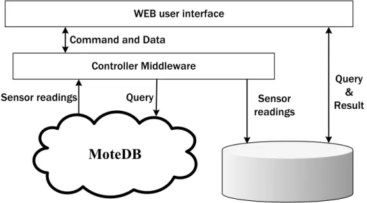
The system overview of ComBase is shown in Fig. 4.1. In ComBase, the sensor nodes are viewed as a virtual database storing sensor reading with different space, different time, and different resolution. Processing nodes at highest level periodically reports the compressed data to the controller middleware, then the controller middleware writes these data to the physical database. Users can query data of the sensing field through internet. The WEB user interface is connected to the database directly. Since only processing nodes at highest level will report data to the controller middleware, the database only possesses data from processing nodes at highest level. If the query is targeted to sensor or processing nodes at lower levels, the controller middleware will send query messages to acquire data with higher precision. The result will be shown on the user interface and stored in database. Thus, next time when these data are queried, no extra query and transmission of data will be invoked.
com-WEB user interface
Controller Middleware Command and Data
MoteDB
Sensor readings Query
Sensor Reading Database Sensor
readings
Query & Result
Figure 4.1: MoteBase architecture.
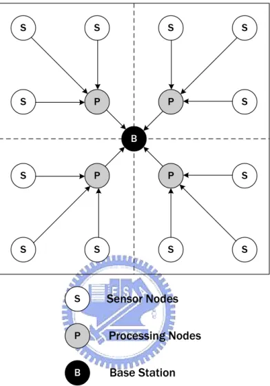
pliant module allowing lowpower operations and offering a 250-Kbps data rate. In our experi-ment, we deploy 17 micaz motes in a 4 × 4 squares with 12 motes being sensor nodes ,4 motes being processing nodes, and one mote being the sink. The scenario is shown in fig XX. In this scenario, the size of a macro-block is 4. A processing node will collect sensor readings from 3 sensor nodes and compress these data with its own sensor readings. The controller middleware will decompress these data and the results will be shown on the WEB user interface. Besides monitoring the current status of the sensing field, users can query the database and ComBase for sensor readings with higher precision and old sensor readings.
We deployed the system with spatial compression algorithm and temporal compression algorithm in a meeting room and measure the temperature to compare its data accuracy and number of transmission with the straightforward data reporting method. The topology of our network is shown Fig. 4.2, and the reporting routes of straightforward data reporting method fol-low the arrows in Fig. 4.2. The reporting interval is ten minutes, and the experiment lasts eight
hours, and the threshold of temporal compression algorithm is 0.5 centigrade. We choose the compression rate as 75% in spatial compression algorithm. The packet size of sensor reading reporting packets is 15 bytes with 11 bytes being header and trailer and 4 bytes being payloads. The packet size of compressed data is 19 bytes with 11 bytes being header and trailer and 8 bytes being payloads. For processing nodes in straightforward reporting method, forwarding every packets from its sensor nodes wastes a lot bandwidth because of the redundant packet header. The processing nodes will wait for merge sensor readings from its children to reduce the number of packets and the redundant header at the same time. The packet size from processing nodes to base station is 21.
The experimental results are shown if Fig. 4.3. In Fig. 4.3 (a), the decompressed data after temporal compression algorithm and temporal compression algorithm is close to the real en-vironment. The the average error is 0.4853 centigrade, but the sum of decompressed sensor readings at each interval is very close to that of reading reading. Fig. 4.3 (b) shows the number of transmission of straightforward data reporting method and our compression algorithms. The number of packet is constant in straightforward is constant even if the environment changes slightly. In our data compression algorithms, since temporal compression algorithm exploits temporal data correlation well and spatial compression algorithm reduce the number of less important data. The result shows our algorithms performs much better than that of straightfor-ward data reporting. The number of transmission is only 33% of that of straightforstraightfor-ward data reporting. To conclude, our data compression algorithms achieve the goal of reducing energy consumption while maintains good data accuracy at the same time.
The snapshot of the system is shown in Fig. 4.4. The system includes two parts: wireless sensor network and web and database server. The topology of these micaz motes follows is shown in Fig. 4.2. The web and database server will stores the received sensing reading and
S S S P B S S S P S S S P S S S P S P B Sensor Nodes Processing Nodes Base Station
Figure 4.2: Implementation Scenario.
˃ ˄˃˃˃ ˅˃˃˃ ˆ˃˃˃ ˇ˃˃˃ ˈ˃˃˃ ˉ˃˃˃ ˊ˃˃˃ ˋ˃˃˃ ˌ˃˃˃ ˄ˊˍˇ ˈ ˄ˋˍˆ ˃ ˄ˌˍ˄ ˈ ˅˃ˍ˃ ˃ ˅˃ˍˇ ˈ ˅˄ˍˆ ˃ ˅˅ˍ˄ ˈ ˅ˆˍ˃ ˃ ˅ˆˍˇ ˈ ˃˃ˍˆ ˃ ˃˄ˍ˄ ˈ ˡ̈̀˵˸̅ʳ̂˹ʳ̃˴˶˾˸̇̆ ˧ ˼̀ ˸ ˦̇̅˴˼˺́̇ʳ˙̂̅̊˴̅˷ ˥˸̃̂̅̇˼́˺ʳˠ˸̇˻̂˷ ˥˸̃̂̅̇˼́˺ʳ̊˼̇˻ʳ˧˗˖ˠ ˴́˷ʳ˦˗˖ˠ ˅ˊ ˅ˊˁˈ ˅ˋ ˅ˋˁˈ ˅ˌ ˅ˌˁˈ ˆ˃ ˆ˃ˁˈ ˄ˊ ˍˇ ˈ ˄ˋ ˍ˄ ˈ ˄ˋ ˍˇ ˈ ˄ˌ ˍ˄ ˈ ˄ˌ ˍˇ ˈ ˅˃ ˍ˄ ˈ ˅˃ ˍˇ ˈ ˅˄ ˍ˄ ˈ ˅˄ ˍˇ ˈ ˅˅ ˍ˄ ˈ ˅˅ ˍˇ ˈ ˅ˆ ˍ˄ ˈ ˅ˆ ˍˇ ˈ ˃˃ ˍ˄ ˈ ˃˃ ˍˇ ˈ ˃˄ ˍ˄ ˈ ˧˸̀̃˸̅˴̇̈̅˸ ˧ ˼̀ ˸ ˥˸˴˿ʳ˦˸́̆̂̅ʳ˥˸˴˷˼́˺̆ ˗˸˶̂̀̃̅˸̆̆˸˷ʳ˦˸́̆̂̅ (a) (b)
display the newly received sensing reading by the means of web. Fig. 4.5 denotes the user interface of the implementation of MRCQ. This is a web user interface that users can access data from remote sensors and control these sensors through the user interface. The upper portion is information of the 16 deployed sensors, including their number, location, and status, and the sensed temperature, which is denoted by blue numbers. The temperature of sensors is updated every 15 seconds. The green light/red circle denote the status of a sensor. If a red light appears, this means this sensor is inactive. The middle part of the web user interface is flow statistics. This part shows flow size without any compression, flow size with spatial compression and flow size with spatial and temporal compression at the same time. Initially, no data compression algorithm is used to reduce the flow size. Users can turn on functions of spatial compression and temporal compression through the web user interface and observe the difference of flow size. The lower part of the user interface is query field. In the query field, users can specify the query conditions, including the time, location and data source. If the data source is from sensing reading database, no query is injected into WSNs. The database will response the query according to the local database. Note that the database can only supply the sensing reading with larger error because the characteristics of spatial compression. Data with higher precision must be required from WSNs. Therefore, users can select the data source option as ”from wireless sensor networks” to query the WSNs.
Sensing Reading Database and
Web Server Processing
Nodes
Flow Statistics
Spatial compression function: Temporal compression function:
In past 15seconds:
Turn On
Reporting without compression: receives 28packets * 17bytes = 476bytes
Reporting with spatial compression: receives 280bytes,flow reduction:41.18%
Reporting with spatial compression: receives 49bytess,flow reduction:89.71%
Turn On
Query Field:
Select the query range of sensors
x: to y: to
Data Filter:
No limitaton
Select the Range 20 (centigrade) to 30 (centigrade)
Data Source:
From Sensor Networks
Select Query Time Type:
Continuous: 5 minutes age to 10 minutes age Instant: 5 minutes age
1(0,0) 2(1,0) 3(0,1) 4(1,1) 5(2,0) 6(3,0) 7(2,1) 8(3,1) 9(0,2) 10(1,2) 11(2,2) 12(3,2) 13(0,3) 14(1,3) 15(2,3) 16(3,3) 27.3759 27.3759 27.442 27.691 27.442 27.2742 27.3759 27.6114 27.442 27.6941 27.9471 27.3759 27.6114 27.442 27.1908 27.1908 Information of a sensor node Switches of Spatial Compression and Temporal Compression Flow Statistics Query Conditions
Chapter 5
Simulation
In previous section, we have demonstrated our Multi-resolution query system. Due to the lim-itation of number of devices, we cannot do experiments with larger scale. In this section, we evaluate the performance of our system, such as data error rate and the flow amount by simula-tion.
In our simulation, we randomly scatter 1000 sensors into a sensing field with size 256 feet × 256 feet. The transmission range of these nodes are identical, and we select 20 feet as the transmission rage. There are 21 nodes elected as the processing nodes, with 20 level 1 processing nodes, 4 level 2 processing nodes, and 1 serves as the sink. In the following experiments, we will evaluate data amount and error rate. The data amount is the sum of total bytes transmitted in the WSNs. The sum of header and trailer length of a packet is 8 bytes, and the payload of each compressed data packet is 28 bytes, and that of a sensor reporting is 2 bytes. The error rate er is defined as follows:
er = 1 N2 N −1X i=0 N −1X j=0
|Mdecomp[i, j] − Mreal[i, j]|
Mreal[i, j]
Where Mdecomp[i, j] represents the decompressed Matrix by sink, and Mdecomp[i, j]
repre-sents the real reading at cell [i, j].
Our system is used to sense the environment. Before we start the simulation, we should generate datasets for experiment first. In order to evaluate the precision of the decompressed data after SDCA and TDCA, we generate virtual events in our simulation. The event sensing reading r(x, y) at location (x, y) is represented as:
r(x, y) = rnormal+ rf luc+ max e(x, y) (5.2)
where rnormalis the default sensing reading, rf lucis the tiny fluctuation of sensing readings,
and e(x, y) is the value that a sensor at (x, y) influenced by nearby events. For an event, the reading at (x, y) influenced by this event is:
e(x, y) =
½
amp × (top − grad ∗ ((xevent− x)2+ (yevent− y)2))
0 if e(x, y) < 0
where top (xevent, yevent) is the center of this event, and the maximum sensing reading of
this event shows at (xevent, yevent), with the value being top. The sensing readings decay as
the distance between (xevent, yevent) and (x, y) increases, and the grad defines the rate that the
sensing readings decay. amp is the degree of the event. For an event, a larger amp means this event poses larger impact. amp is one of the variable condition in our simulation. Finally,
r(x, y) is decided by rnormal, rf lucand the maximum of e(x, y). In our simulations, we choose
the number of events as a random number between 1 to 8.
Fig. 5.1 shows the data error rate under different degree of events. The simulation results show that larger degrees of events cause higher error data rate. SDCA tends to keep data with
˃ ˈ ˄˃ ˄ˈ ˅˃ ˃ ˄ ˅ ˆ ˇ ˈ ˉ ˊ ˘́̉˼̅̂́̀˸́̇ʳ˩˴̅˼˴́˶˸ ˔ ̉˸ ̅˴ ˺˸ ʳ˘ ̅̅ ̂̅ ʳ˥ ˴̇ ˸ʳ ʻʸʼ ˖̂̀̃̅˸̆̆˼̂́ʳ˥˴̇˸ˍʳˆ˃ʸ ˖̂̀̃̅˸̆̆˼̂́ʳ˥˴̇˸ˍʳˈ˃ʸ ˖̂̀̃̅˸̆̆˼̂́ʳ˥˴̇˸ˍʳˊ˃ʸ ˖̂̀̃̅˸̆̆˼̂́ʳ˥˴̇˸ˍʳˌ˃ʸ
Figure 5.1: Data error rate under different degree of events (amp)
higher similarity. Larger degree of events causes the sensing readings much larger than that of a default reading. Compared with default sensing readings, the number of sensing readings under influence of events are minority that their readings are lowered during the compression procedure. ˉ˃˃˃ ˊ˃˃˃ ˋ˃˃˃ ˌ˃˃˃ ˄˃˃˃˃ ˄˄˃˃˃ ˄˅˃˃˃ ˆ˃ ˇ˃ ˈ˃ ˉ˃ ˊ˃ ˋ˃ ˌ˃ ˖̂̀̃̅˸̆̆˼̂́ʳ˥˴̇˸ ˙˿ ̂̊ ʳ˴ ̀ ̂̈ ́̇ ʳʻ ˵̌ ̇˸ ʼ ˅ ˅ˁˈ ˆ ˆˁˈ ˇ ˇˁˈ ˈ ˈˁˈ ˉ ˉˁˈ ˊ ˘ ̅̅̂ ̅ʳ ̅˴ ̇˸
Figure 5.2: Data error rate v.s. Flow amount
rate decreases as the compression rate increases. The higher the compression rate, the more data are available to decompress. The flow amount increases with compression rate. High compression rate can reduce the energy consumption, but the high error rate makes the data untrustful. On the other hand, low compression rate helps to reduce the error rate, but it requires large amount of transmission. The intersection of these two lines lays between compression rate of 60 percentage to 70 percentage. Compression rate at this interval can reduce the total energy consumption while maintains acceptable data rate.
Chapter 6
Conclusion
In this paper, we proposed data compression algorithms suitable for monitoring applications of WSNs. We also implemented a query system exploiting these data compression algorithms and do some experiments on measuring temperature in laboratory using micaz motes . Exper-imental results indicates our system can largely prolong the system life time. Our experiments are small scale because of equipment limitation. Our future work is evaluating system perfor-mance bye simulations. Furthermore, we are modifying temporal data compression algorithm for automatically adapt the update threshold to arise the data accuracy.
Bibliography
[1] N. Ahmed, T. Natarajan, and K. R. Rao, “Discrete cosine transfom,” IEEE Transactions
on Computers, vol. 1, no. C-23, pp. 90–93, 1974.
[2] I. F. Akyildiz, W. Su, Y. Sankarasubramaniam, and E. Cayirci, “A survey on sensor net-works,” IEEE Communications Magazine, vol. 40, no. 8, pp. 102–114, 2002.
[3] A. Amis, R. Prakash, T. Vuong, and D. Huynh, “Max-min d-cluster formation in wireless ad hoc networks,” in INFOCOM 2000, vol. 1, 2000, pp. 32–41.
[4] Crossbow, “MOTE-KIT2400 - MICAz Developer’s Kit,” http://www.xbow.com.
[5] G. Davis, “Wavelet image compression construction kit,”
http://www.geoffdavis.net/dartmouth/wavelet/wavelet.html.
[6] C. T. Ee and R. Bajcsy, “Congestion control and fairness for many-to-one routing in sensor networks,” in ACM International Conference on Embedded Networked Sensor Systems, 2004, pp. 148–161.
[7] K. W. Fan, S. Liu, and P. Sinha, “Structure-free data aggregation in sensor networks,”
[8] D. Ganesan, D. Estrin, and J. Heidemann, “Dimensions: why do we need a new data handling architecture for sensor networks?” ACM SIGCOMM Computer Communication
Review, vol. 33, no. 1, pp. 143–148, 2003.
[9] D. Ganesan, B. Greenstein, D. Estrin, J. Heidemann, and R. Govindan, “Multiresolution storage and search in sensor networks,” ACM Transactions on Storage, vol. 1, no. 3, pp. 277–315, 2005.
[10] D. Ganesan, B. Greenstein, D. Perelyubskiy, D. Estrin, and J. Heidemann, “An evaluation of multi-resolution storage for sensor networks,” in ACM International Conference on
Embedded Networked Sensor Systems, 2003, pp. 89–102.
[11] W. B. Heinzelman, A. P. Chandrakasan, H. Balakrishnan, and C. MIT, “An application-specific protocol architecture for wireless microsensor networks,” Wireless
Communica-tions, IEEE Transactions on, vol. 1, no. 4, pp. 660–670, 2002.
[12] S. Helal, W. Mann, H. El-Zabadani, J. King, Y. Kaddoura, and E. Jansen, “The gator tech smart house: a programmable pervasive space,” IEEE Computer, vol. 38, no. 3, pp. 50–60, 2005.
[13] C. Intanagonwiwat, R. Govindan, and D. Estrin, “Directed diffusion: a scalable and ro-bust communication paradigm for sensor networks,” in ACM International Conference on
Mobile Computing and Networking, 2000, pp. 56–67.
[14] S. Lindsey, C. Raghavendra, and K. M. Sivalingam, “Data gathering algorithms in sensor networks using energy metrics,” IEEE Transactions on Parallel and Distributed Systems, vol. 13, no. 9, pp. 924–935, 2002.
[15] S. Madden, M. J. Franklin, J. M. Hellerstein, and W. Hong, “TAG: a tiny aggregation service for ad-hoc sensor networks,” ACM SIGOPS Operating Systems Review, vol. 36, pp. 131–146, 2002.
[16] S. Nath, P. B. Gibbons, S. Seshan, and Z. R. Anderson, “Synopsis diffusion for robust ag-gregation in sensor networks,” in ACM International Conference on Embedded Networked
Sensor Systems, 2004, pp. 250–262.
[17] M. Nelson and J. L. Gailly, The data compression book (2nd edition). MIS:Press, New
York, USA, 1996.
[18] W. B. Pennebaker and J. L. Mitchell, JPEG: still image data compression standard. Van Nostrand Reinhold, New York, USA, 1993.
[19] C. C. Y. Poon, Y. T. Zhang, and S. D. Bao, “A novel biometrics method to secure wire-less body area sensor networks for telemedicine and m-health,” IEEE Communications
Magazine, vol. 44, no. 4, pp. 73–81, 2006.
[20] R. M. Rao and A. S. Bopardikar, Wavelet transforms: introduction to theory and
applica-tions. Addison Wesley Publications, 1998.
[21] J. A. Storer, Data compression: methods and theory. Computer Science Press, New
York, USA, 1988.
[22] R. Szewczyk, E. Osterweil, J. Polastre, M. Hamilton, A. Mainwaring, and D. Estrin, “Habitat monitoring with sensor networks,” Communications of the ACM, vol. 47, no. 6, pp. 34–40, 2004.
[23] Y. C. Tseng, Y. C. Wang, K. Y. Cheng, and Y. Y. Hsieh, “iMouse: an integrated mobile surveillance and wireless sensor system,” IEEE Computer, vol. 40, no. 6, pp. 60–66, 2007.
[24] M. Vetterli and J. Kovacevic, Wavelets and subband coding. Prentice Hall, New Jersey, USA, 1995.
[25] Y. Xue, Y. Cui, and K. Nahrstedt, “Maximizing lifetime for data aggregation in wireless sensor networks,” Mobile Networks and Applications, vol. 10, no. 6, pp. 853–864, 2005.