正交多頻多工系統使用複雜度資訊之位元寬度決定法

全文

(1)國立交通大學電子工程學系電子研究所碩士班. 碩士論文. 正交多頻多工系統使用複雜度資訊之位元寬度決定法 Bit Width Determination Using Complexity Information for OFDM system. 研究生：陳彥宇指導教授：周景揚. 中華民國九十七年八月. 博士.

(2) 正交多頻多工系統使用複雜度資訊之位元寬度決定法 Bit Width Determination Using Complexity Information for OFDM system 研究生：陳彥宇. Student：Yen-Yu Chen. 指導教授：周景揚博士. Advisor：Dr. Jing-Yang Jou. 國. 立. 交. 電子工程學系碩. 士. 通. 大. 學. 電子研究所碩士班論. 文. A Thesis Submitted to Department of Electronics Engineering & Institute of Electronics College of Electrical and Computer Engineering National Chiao Tung University in Partial Fulfillment of the Requirements for the Degree of Master in Electronics Engineering August 2008 HsinChu, Taiwan, Republic of China. 中華民國九十七年八月.

(3) Bit Width Determination Using Complexity Information for OFDM System Student: Yen-Yu Chen. Advisor: Dr. Jing-Yang Jou. Department of Electronics Engineering Institute of Electronics National Chiao Tung University. Abstract An automatic algorithm using complexity information for the floating point to fixed point conversion is proposed. The goal of the proposed algorithm is to minimize the hardware complexity and reduce the simulation times. The algorithm considers both the integer bit width and the fraction bit width. For the integer bit width, the algorithm identifies numbers of the integer bit width to prevent the overflow. For the fraction bit width, the algorithm uses the lower bound and the upper bound to find the results. We apply the proposed algorithm to the OFDM system. The results show that the proposed algorithm reduces almost 30% simulation time than complexity-and-distortion measure and sequential search method.. i.

(4) 正交多頻多工系統使用複雜度資訊之位元寬度決定法研究生：陳彥宇. 指導教授：周景揚博士. 國立交通大學電子工程學系電子研究所碩士班. 摘要我們提出使用複雜度資訊的自動化轉換浮點數到固定點數演算法，演算法的目標是縮小硬體複雜度並且同時減少模擬時間。我們提出的演算法同時考慮到了整數以及小數的位元寬度。對整數的位元寬度來說，演算法決定需要多少位元寬度以避免溢位。對小數位元寬度來說，我們提出的演算法使用上邊界以及下邊界來得到最後的結果。我們把提出來的演算法應用在正交多頻多工系統上面。結果顯示提出來的演算法比循序搜尋法以及複雜度誤差度量測法減少大約 30%的摹擬時間。. ii.

(5) Acknowledgment First of all, I would like to express my sincere gratitude to my advisor Professor Jing-Yang Jou for his suggestions and guidance throughout the years. Second, I would also like to give my gratitude to my co-guidance advisor Professor Lan-Da Van for his guidance. He always provides his opinions unselfishly to improve my research quality. Third, I would like to thank Cheng-Yeh Wang and Zwei-Mei Lee. Without their help, I could not finish my work. Fourth, I would also like to thank Geeng-Wei Lee. He always gives me the biggest support when I am down. Fifth, I would like to thank Minna Lo, she is always with me through all the happiness and sorrow. Special thanks to all EDA lab members for their company and friendship. Finally, I would like to express my sincere gratitude to my family and all my friends for the support and encouragement.. iii.

(6) Content 摘要................................................................................................................................ii Acknowledgment ......................................................................................................... iii Content..........................................................................................................................iv List of Tables.................................................................................................................vi List of Figures ..............................................................................................................vii Chapter 1 Introduction ...................................................................................................1 1.1 Technology Trend ............................................................................................1 1.2 Analytic Approach ...........................................................................................2 1.3 Simulation-based Approach .............................................................................1 1.4 Motivation........................................................................................................2 1.5 Thesis Organization .........................................................................................2 Chapter 2 Preliminary ....................................................................................................3 2.1 The OFDM System ..........................................................................................3 2.2 Floating Point and Fixed Point ........................................................................5 2.2.1 Floating Point........................................................................................5 2.2.2 Fixed Point ............................................................................................6 2.3 Problem Formulation .......................................................................................8 2.4 Previous Works ................................................................................................9 Chapter 3 Proposed Algorithm.....................................................................................13 3.1 Fixed Point Bit Width Determination ............................................................13 3.2 Upper Bound Determination..........................................................................15 3.3 Lower Bound Determination .........................................................................17 3.4 Fine Tuning Process.......................................................................................19 iv.

(7) 3.4.1 First Stage ...........................................................................................19 3.4.2 Second Stage .......................................................................................22 Chapter 4 Experimental Results...................................................................................29 4.1 Experimental Information..............................................................................29 4.2 Experimental Results .....................................................................................31 4.3 Comparison Results .......................................................................................34 Chapter 5 Conclusion and Future Work.......................................................................39 Reference .....................................................................................................................40. v.

(8) List of Tables Table 4.1 Complexity of the receiver...........................................................................30 Table 4.2 Upper bound and lower bound of the all variables ......................................31 Table 4.3 Result of the proposed algorithm .................................................................32 Table 4.4 Upper bound and lower bound of all variables ............................................32 Table 4.5 Simulation result of the proposed algorithm................................................33 Table 4.6 Upper bound and lower bound of the all variables ......................................33 Table 4.7 Result of the proposed algorithm .................................................................34 Table 4.8 Simulation times of two algorithms .............................................................34 Table 4.9 Hardware complexity of two algorithms .....................................................34 Table 4.10 Simulation times of three algorithms .........................................................35 Table 4.11 Hardware complexity of two algorithms....................................................35. vi.

(9) List of Figures Figure 2.1 Transmitter architecture of the OFDM system.............................................3 Figure 2.2 Receiver architecture of the OFDM system .................................................4 Figure 2.3 Channel estimator of the OFDM system ......................................................4 Figure 2.4 Floating point representation........................................................................5 Figure 2.5 Fixed point representation ............................................................................6 Figure 2.6 Complete flow of the algorithm ...................................................................9 Figure 3.1 Flow of bit width determination .................................................................14 Figure 3.2 Upper bound of the algorithm ....................................................................16 Figure 3.3 Lower bound of the algorithm....................................................................18 Figure 3.4 Flow of the first stage of fine tuning process .............................................20 Figure 3.5 Simulated combinations for first stage of fine tuning process ...................21 Figure 3.6 Flow of the second stage of fine tuning process.........................................23 Figure 3.7 Simulated combinations for second stage of fine tuning process...............24 Figure 3.8 Example of the first step of fine tuning first stage .....................................25 Figure 3.9 Example of the second step of fine tuning first stage.................................26 Figure 3.10 Example of the first step of fine tuning second stege...............................27 Figure 3.11 Example of the second sep of fine tuning second stage ...........................28 Figure 4.1 Receiver of the OFDM system ...................................................................29 Figure 4.2 Fine signal detection of receiver.................................................................30 Figure 4.3 Channel estimator of the receiver...............................................................30 Figure 4.4 Comparison result of BER = 0.01 ..............................................................37 Figure 4.5 Comparison result of BER = 0.001 ............................................................37 Figure 4.6 Comparison result of BER = 0.0001 ..........................................................38. vii.

(10) Chapter 1 Introduction 1.1 Technology Trend Most digital signal processing system algorithms are first developed in high level language (such as MATLAB and C) in floating point representation for high precision, but in practical digital hardware implementation, the floating point representation is transferred to the fixed point for low power, area and latency. The procedure of the bit width determination is traditionally made manually. For a complex design, more than 50% of the design time is spent on the floating point to fixed point conversion [1]. Because the floating point to fixed point conversion is done manually, it is time consuming and error prone. There are many approaches developed in several languages for the floating point to fixed point conversion [3], [4]. Optimizing bit width is a NP-hard problem and has been the focus of numerous research contributions [2] in the past decade. Strategies for the floating point to fixed point conversion can be roughly categorized into two groups. One group is the analytic approach, and the other one is the simulation-base approach.. 1.

(11) 1.2 Analytic Approach First strategy is analytic approach. It analyzes the finite bit width effects due to the fixed point arithmetic. The technique introduced in [5] exploits advances in interval representation methods from affine arithmetic and the power of a probabilistic bounding method to dramatically reduce the pessimism of error estimation. The MiniBit is presented in [6]. It also uses affine arithmetic and the analytical error models for range analysis and utilizes the ASA (adaptive simulated annealing) for the precision analysis. The MiniBit+ was proposed in [7]. It combines the interval and affine arithmetic for range analysis. Fang et al. employ affine arithmetic for modeling range and precision analyses [8]. While the use of affine arithmetic to model precision error is demonstrated, the authors do not use it to optimize the actual bit width. Results of analytic approach are obtained in short time, because analytic approach does not have to simulate the system. Although the analytic approach is fast, the results of the analytic approach are considered to be more conservative. However, the analytic approach is not suitable for large systems because numerous loops could make results of signals divergent.. 2.

(12) 1.3 Simulation-based Approach The second strategy is the simulation-based approach. Because results of the analytic approach could be too pessimistic to reduce total hardware, the simulation-based approach monitors the signals of the system to determine the integer bit width and the fraction bit width. Without special care on the large number of loops, the simulation-based approach is better than the analytic approach in complex systems. Some algorithms search optimum bit width without error distortion information [9], [10]. Exhaustive search [9] and branch-and-bound procedure [10] can find an optimum bit width. However, these algorithms have an unrealistic search space as the number of variable increases. C.Y. Wang et al. proposed a hybrid word length determination algorithm [14], but the algorithm only utilizes in the pipelined FFT processors. Babb et al. have developed the BITWISE compiler [11], which determines the precision of all input, intermediate and output signals in a synthesized hardware design from a C program description. Execution time, however, increases exponentially when the number of signal increases.. 1.

(13) 1.4 Motivation As mentioned above, the analytic approach is not suitable for complex systems, so we propose a simulation-based approach to determine the bit width of the OFDM system. S. Roy et al. proposed an algorithm that obtains the uniform bit width first [12](it means every variable has the same fraction bit width), and then further reduces the bit width from the uniform bit width. It only considers the total bit width as the objective cost, but in practical systems the total hardware cost should also consider the functional units. K. Han et al. proposed the sequential search for the word length optimization, but the algorithm only considered the error distortion [17]. Distortion and complexity measure are further proposed by K. Han. Both error distortion and hardware complexity are concurrently considered. The previous two works only increase one bit in each simulation. Here we proposed a new algorithm, which combines the features of previous two algorithms, to reduce the simulation time and the algorithm in term of the error and hardware complexity.. 1.5 Thesis Organization The rest of the thesis is organized as follows. Chapter 2 introduces the OFDM system for our experiment, the difference between the floating point and the fixed point, problem formulation and three algorithms which are closely related to proposed algorithm. In Chapter 3, proposed algorithm is presented in detail. Experimental results are showed in Chapter 4. Finally, the conclusion is made in Chapter 5 2.

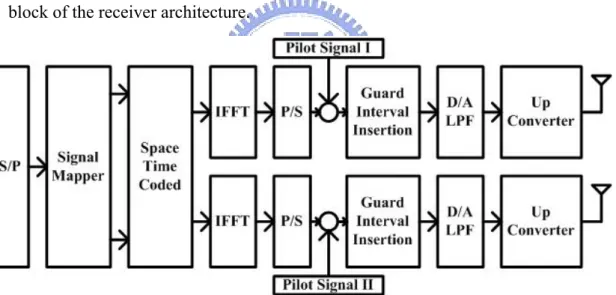
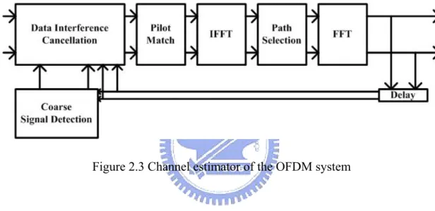
(14) Chapter 2 Preliminary 2.1 The OFDM System The OFDM system used in the case study is obtained from [13]. Figure 2.1, Figure 2.2 and Figure 2.3 depict the OFDM system blocks. Figure 2.1 depicts the transmitter architecture part of the system. Figure 2.2 depicts the receiver architecture part of the system. Figure 2.3 deeply depicts the channel estimator block of the receiver architecture.. Figure 2.1 Transmitter architecture of the OFDM system. 3.

(15) Figure 2.2 Receiver architecture of the OFDM system. Figure 2.3 Channel estimator of the OFDM system. 4.

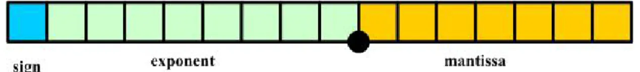
(16) 2.2 Floating Point and Fixed Point There are two ways in numeric representation. One is floating point and the other one is fixed point. Floating point representation has wider range and fixed point has less complexity in hardware implementation.. 2.2.1 Floating Point. Figure 2.4 Floating point representation The floating point representation is showed in Figure 2.4. The bit width of the floating point contains one sign bit, exponent bits and mantissa bits. The name floating point comes from the fact that the radix point can float. It means that the radix point can allocate anywhere relative to the significant digits of the number. The first thing to add or subtract two floating points is to represent them with the same exponent and shift the mantissa bits. Because the exponent bits have to be checked and mantissa bits be shifted, it will be more complicated than fixed point representation in practical hardware implementation.. 5.

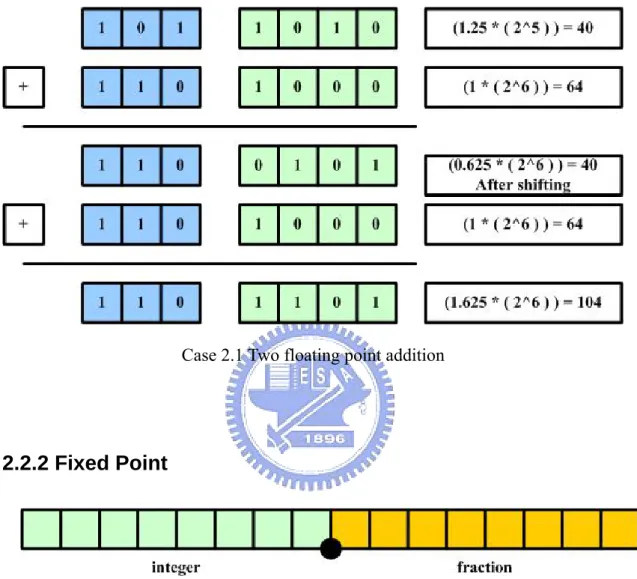
(17) In the Case 2.1 below, the second number is shifted right by two digits, and we process it with the normal addition.. Case 2.1 Two floating point addition. 2.2.2 Fixed Point. Figure 2.5 Fixed point representation The fixed point representation is showed in Figure 2.5. The radix point separates the integer part and fraction part. In contrast to floating point representation, the radix point of fixed point already fixed. It means that the radix point can not move anymore after the bit width determination of the integer part and the fraction part.. 6.

(18) Unlike the addition and subtraction of floating point, the addition and subtraction of fixed point just add or subtract the integer part and the fraction part individually, and with carry out if necessary.. Case 2.2 Two fixed point addition. Two fixed point numbers with the same bits in Case 2.1 is showed in Case 2.2. Because the addition in fixed point representation does not compare the exponent bits and shift the mantissa bits, it needs less hardware than floating point does.. 7.

(19) 2.3 Problem Formulation The bit width is a set of N bit widths of a system and is defined to be a bit width vector as follow:. W = {w1 , w2 ,", wN }.. (2.1). Assume that the objective function f is defined by the sum of every bit width implementation hardware cost function c as N. f (W ) = ∑ ck ( wk ). (2.2). k =1. The error function p indicates the bit error rate and is constrained as below, and Preq is a constant for a required error constraint.. p(W ) ≤ preq. (2.3). The lower bound bit width set is denoted by LB and the upper bound bit width set is denoted by UB. The lower bound and upper bound of each variable are also considered as constraint:. wk _ LB ≤ wk ≤ wk _ UB , ∀k = 1,..., N. (2.4). The complete bit width optimization problem can be stated as:. min f (W ) , subject to p ( w) ≤ pr eq , LB ≤ W ≤ UB. W ∈I N. 8. (2.5).

(20) 2.4 Previous Works S. Roy and P. Banerjee proposed an algorithm to determine the bit width in MATLAB [12]. Figure 2.6 shows the complete flow of the algorithm. First, the algorithm determines the integer bit width. Second, the algorithm generates the fixed point form of MATLAB. Third, the algorithm simulates the floating point version and fixed point version to record the error metric. Fourth, the coarse optimize will be executed to find a rough solution. Finally, the fine optimize will be executed to further minimize the bit width.. Figure 2.6 Complete flow of the algorithm. 9.

(21) The Coarse_Optimize phase of the automatic algorithm follows the divide-and-conquer approach to quickly move closer to the optimal set. They vary the fraction bit width to get a set of coarse optimized fraction bit width, which are all equal. The accuracy of the output of an algorithm is less sensitive to some internal variables than to others. Hence, starting from the coarse optimal point, they apply Fine_Optimize algorithm to the coarse optimized variables. They do not perform finer optimization directly from the start because it will take a long time to converge. The Fine_Optimize algorithm basically tries to find out the variable whose impact on the quantization error is the smallest and to reduce fraction bit width in such variables as long as the error is within the EM constraint. Then, it tries to find a variable whose impact on the error is largest and increase one fraction bit while simultaneously reducing two bits in the variable with the smallest impact on the error, thereby reducing one bit overall. It performs such bit reductions iteratively until the EM constraint is exceeded. The algorithm only reduces the complexity by choosing the total bit-width as the objective function. The impact of bit-width on area should depend on the functional unit.. 10.

(22) K. Han et al. proposed sequential search for word length optimization [17]. The basic notion of sequential search is that each trial eliminates a portion of the region being search. The sequential search method decides where the most promising areas are located, and continues in the most favorable region after each set of simulations. The principles of sequential search in n dimensions can be summarized in the following four steps: 1.. Select a set of feasible values for the independent variables, which satisfy the desired performance during one-variable simulation. This is a base point.. 2.. Evaluate the performance at the base point.. 3.. Choose the feasible locations at which evaluate the performances and compare their performance. 4.. If one point is better than others, move to the better point, and repeat the search, until the point has been located to within the desired accuracy.. The sequential search only considers the error distortion and does not consider the hardware complexity, either. Therefore, K. Han and B.L.Evans further proposed the complexity and distortion measure for the bit width determination [16].. 11.

(23) The complexity-and-distortion measure combines the hardware complexity measure with the error distortion measure by a weighted factor. In the objective function, both hardware complexity and error distortion are simultaneously considered. They normalize the hardware complexity and the error distortion function by multiply them with hardware complexity and error distortion weighting factors respectively. Setting the hardware complexity and error distortion weighted factor from 0 to 1, the complexity and distortion method searches for an optimum word length with tradeoffs between only hardware complexity measure and error distortion measure method. The complexity-and-distortion measure method can reduce the number of iterations for searching the optimum word lengths, because the error distortion sensitivity information is utilized. This method can more rapidly find the optimum word length that satisfies the required error constraint by using fewer iteration compared to the complexity measure method. However the word lengths are not guaranteed to be optimal in terms of the hardware complexity.. 12.

(24) Chapter 3 Proposed Algorithm 3.1 Fixed Point Bit Width Determination In digital system, there are two numeric representations, floating point and fixed point. Floating point representation allocates one sign bit and a fixed number of bits to exponent and mantissa. In fixed point representation, the bit width is divided for the integer part and the fraction part. When designers develop high-level algorithms, floating-point formats are usually used because of its accuracy. Floating point representation can present very large range. In hardware, the floating point representation needs to normalize the exponents of the operands and it costs lots of hardware. Floating point representation is usually transferred to fixed point representation to reduce the total hardware cost. As mentioned above, fixed point representation is composed of the integer part and the fraction part. The number of bits assigned to the integer part is called integer bit width (IBW), and the number of bits assigned to the fraction part is called fraction bit width (FBW). The complete fixed point bit width can be represented as:. BW = IBW + FBW.. 13.

(25) Figure 3.1 Flow of bit width determination The total bit width determination procedure is showed in Figure 3.1. First of all, the integer bit width is calculated to prevent overflow. Then, the iteration procedure is used to minimize the fraction bit width to reduce the total hardware cost. The integer bit width has to be long enough to prevent overflow. By monitoring the signals of the system, the minimum and the maximum value of the signals are obtained, and the integer bit width can be also obtained.. Integer bit width = log2 (max (|MAX|, |MIN|)) + 2. After assigning the integer bit width, there are three steps to determine the fraction bit width. First, the uniform fraction bit width is determined to be the upper bound of the algorithm. Second, the individual minimum bit width of every variable is calculated to be the lower bound. Finally, the bit width will be fine tuned between the upper bound and the lower bound for each variable.. 14.

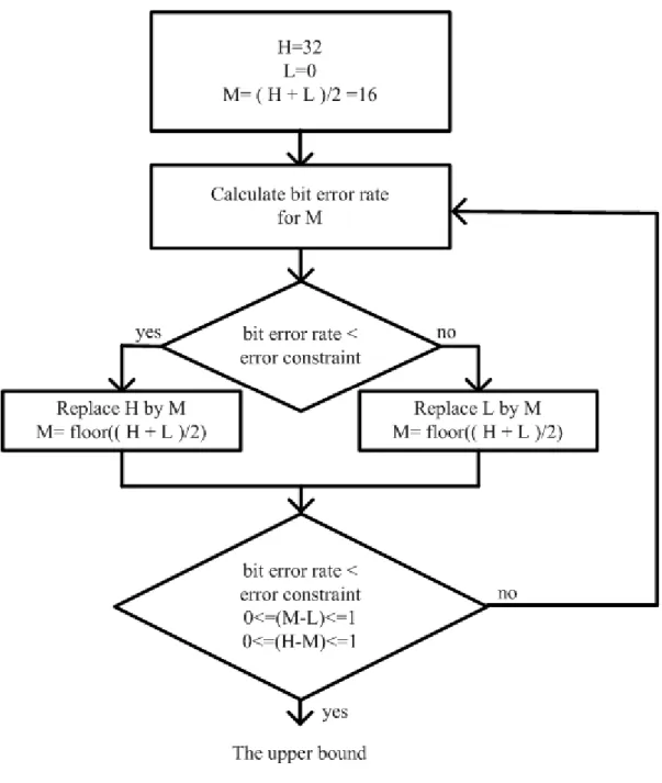
(26) 3.2 Upper Bound Determination In order to accelerate the fraction bit width determination procedure, the uniform fraction bit width is calculated to be the upper bound. The uniform fraction bit width means that every variable has the same fraction bit width. A binary search approach is used to quickly obtain the uniform fraction bit width.. Upper-Bound-Determination ( UB, error_ constraint ) begin 1.. Set H to highest bit width and set L to lowest bit width, M = ( H + L)/2;. 2.. Calculate the BER for all variables having the M fraction bits;. 3.. While ( !(( BER < error_constraint ) and (0 ≤ M-L ≤ 1) and (0≤ H-M ≤1) ) ). 4.. if (BER < error_constraint ). 5.. replace H by M, M = floor (( H + L)/2 );. 6.. else. replace L by M, M = floor(( H + L)/2 );. 7.. Calculate the BER for all variables having the M fraction bits;. 8.. for ( j from 1 to N ). 9.. UB[j] ← M;. 10. return UB; end;. 15.

(27) Figure 3.2 Upper bound of the algorithm The uniform fraction bit width determination procedure is showed in Figure 3.2. The fraction bit width determination procedure will repeat until it meets the condition. We obtain a uniform bit width set which is denoted by UB and the upper bound of every variable. The upper bound of the jth variable is denoted by wj_UB. Because the fraction bit width determination procedure uses binary search approach, it will not spend too much time to find the uniform fraction bit width.. 16.

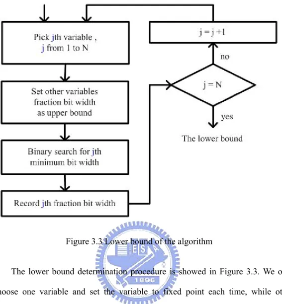
(28) 3.3 Lower Bound Determination In order to minimize the total hardware cost, it has to determine the minimum individual fraction bit width when other variables remain as upper bound. The individual minimum fraction bit width will be the lower bound, and the fine tuning process will start from the lower bound.. Lower-Bound-Determination ( W, UB, LB, error_constraint ) begin 1.. for ( i from 1 to N). 2.. for ( j from 1 to N ). 3.. if ( j != i ). 4. 5.. Set WLB[j] as UB[j];. LB[i] ← minimum_bit_width( WLB, error_constraint); return LB;. end;. 17.

(29) Figure 3.3 Lower bound of the algorithm The lower bound determination procedure is showed in Figure 3.3. We only choose one variable and set the variable to fixed point each time, while other variables remain as upper bound. We use the binary search to find the minimum bit width of the variable. We determine every variable in order and finally obtain a lower bound bit width set, which is denoted by LB. The lower bound of jth variable is denoted by wj_LB. Because the determination procedure uses the binary search for the minimum individual fraction bit width as well, the minimum individual fraction bit width, which will be the start point of fine tuning process, is obtained quickly.. 18.

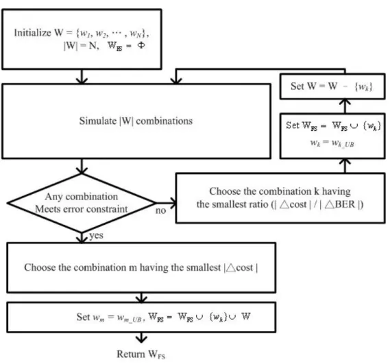
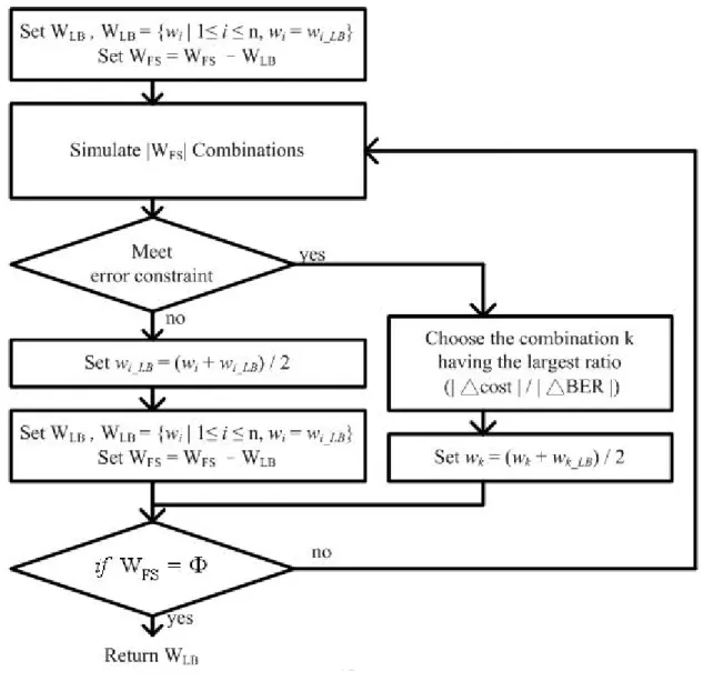
(30) 3.4 Fine Tuning Process 3.4.1 First Stage There are two stages of the fine tuning processes, the first stage will increase the fraction bit width to meet the error constraint, and the second stage will reduce the fraction bit width to reduce hardware complexity under error constraint. In the first stage, after obtaining the lower bound and the upper bound of the fraction bit width, there is a bit width set which all variables are set to their lower bound, and the bit width set will be the first candidate. First of all, the candidate will be simulated and the bit error rate will be recorded. If the bit error rate of the candidate meets the error constraint, it means the candidate is the minimum bit width set so the fine tuning process will be terminated. If the bit error rate of the candidate does not meet the error constraint, it means that the candidate is not long enough to represent the value exactly and the candidate has to be increased. Second, only the bit width of one variable in the candidate is set to the upper bound each time while other variables do not change, and each bit width sets is called one combination. Those combinations will be simulated. There will be n bit-error-rate and hardware cost first, and all of the combinations will be checked to find out if any combination meets the error constraint. Third, if there are more than one combinations meet the error constraint, the combination which has the smallest △cost will be chosen to be new candidate. △cost denotes the difference of the hardware cost between the combination and the candidate. The smallest △cost indicates the variable of combination increases the smallest hardware cost. 19.

(31) Finally, if no combination meets the error constraint, the combination which has the smallest ratio ( | △cost | / | △BER | ) will be chosen to be the new candidate. △ BER denotes the difference of the bit error rate between the combination and the candidate. The smallest ratio ( | △cost | / | △BER | ) means that the combination increases the smallest hardware cost in the same bit error rate. The combination which has the smallest ratio will not be simulated next time, because the variable of the combination already be the upper bound and can not increase anymore. The procedure will repeat from the second step and simulate the combinations until any combination meets the error constraint. The total flow is showed in Figure 3.4 below.. Figure 3.4 Flow of the first stage of fine tuning process. 20.

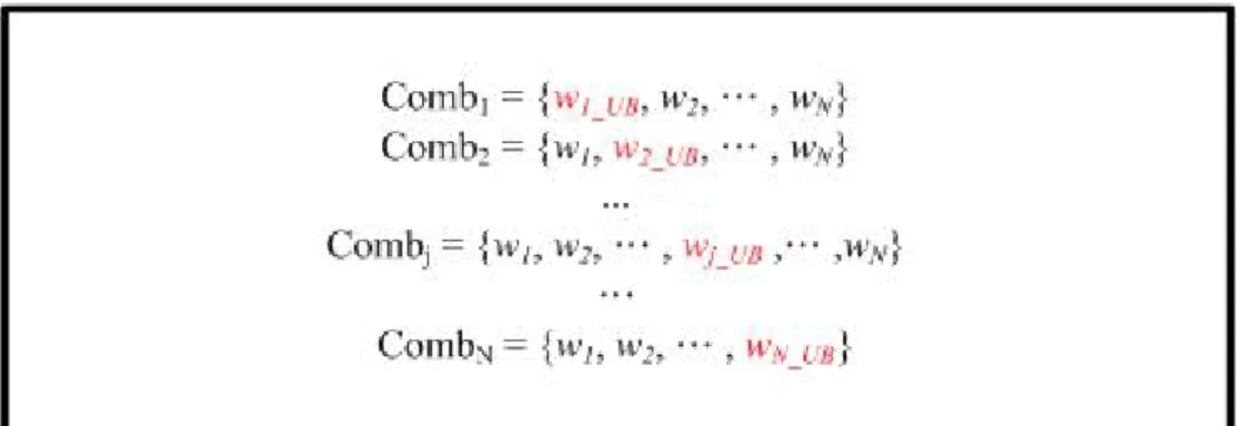
(32) Figure 3.5 Simulated combinations for first stage of fine tuning process W denotes the bit width set of variables. WFS is an empty set. wj represents the bit width of jth variable. There are N variables in the system. The bit width set of the W and WFS will be the candidate. We simulate |W|, which means the number of variable in the set, combinations. Figure 3.5 shows an example of the simulating |W| combinations first time. We only set the bit width of one variable in the W to the upper bound and other variables remain the same bit width. Every bit width set is one combination. After simulating |W| combinations, if there is no combination meeting the error constraint, we choose the combination k having the smallest ratio ( | △cost | / | △BER | ). We set wk to the upper bound and put wk into the WFS, it means wk can not increase anymore. We remove wk from W so that it reduces one simulation next time. If there are more than one combination meeting the error constraint, we choose the combination m having the smallest | △cost |. We set wm to the upper bound and put wm and the rest variables of W into WFS. WFS denotes the variables which already meet the upper bound (from wk and wm) and the variables which remain the lower bound (from W). Now, WFS is the bit width set which meets the error constraint.. 21.

(33) 3.4.2 Second Stage After first stage of the fine tuning process, the candidate already met error constraint. The second stage will reduce the fraction bit width under error constraint in order to minimize the hardware cost. First, the every variable is set to half of sum of the lower bound and the bit width of the candidate, each bit width set is one combinations. We simulate the combinations. Second, if any combination meets the error constraint, the combination which has the biggest ratio ( | △cost | / | △BER | ) are chosen. It means that the variable of the combination has the biggest hardware cost in the same bit error rate. For the combinations which do not meet the error constraint, the lower bounds of these combinations are updated to half of sum of the original lower bound and the bit width of the variables in the combinations. We repeat the procedure until the lower bound could not update anymore. Finally, if the bit width set of the candidate is equal to lower bound, it means that the bit width could not be further reduced. We terminate the second stage of the fine tuning process and obtain the final result.. 22.

(34) Figure 3.6 Flow of the second stage of fine tuning process. The total flow of the second stage of fine tuning process is showed in Figure 3.6 above. WLB denotes the variables which are equal to lower bound. Because the variables in WLB are already equal to lower bound, the bit width of these variables can not reduce anymore and we remove these variables from W. Figure 3.7 shows the combinations for the second stage of fine tuning process. Like first stage of fine tuning process, we only set one variable to half of sum of bit width of variable and its lower bound while other variables remain the same. Each bit width set is one combination. 23.

(35) Figure 3.7 Simulated combinations for second stage of fine tuning process Subsequently, we simulate |W| combinations. If there is more than one combination meeting the error constraint, we choose the combination k having largest ratio ( | △cost | / | △BER | ) and set wk to (wk + wk_LB) / 2. The variables in the combinations which meet the error constraint but have smaller ratio than combination k remain the same bit width in WFS. If combinations do not meet the error constraint, we set the lower bound of the changed variable in the combinations to half of sum of bit width of variable and its lower bound. We will check if there is variable equal to its lower bound. If it is, we remove the variable from |W| and put it into WLB. Finally we will check if W is an empty set. If the W is an empty set, it means that W can not reduce anymore and we terminate the process. Otherwise, we repeat the procedure until the W is equal to lower bound.. 24.

(36) Figure 3.8 Example of the first step of fine tuning first stage The first stage of fine tuning process is showed in Figure 3.8. The figure indicates that there is no combination which meets the error constraint. Since there is no combination meeting the error constraint, the combination which has the smaller ratio ( | △cost | / | △BER | ) will be picked to be the new candidate. The procedure repeats because the bit error rate of new candidate does not meet the error constraint.. 25.

(37) Figure 3.9 Example of the second step of fine tuning first stage. The combination meets the error constraint in the first stage of the fine tuning process showing in Figure 3.9. After first choice of the combination, there are only two combination and the combinations are individually simulated. In these two combinations, only the first combination meets the error constraint. Even if the second combination has the smaller ratio ( | △cost | / | △BER | ), it does not meet the error constraint, so the first combination is chosen to be the new candidate and go to the second stage of fine tuning process.. 26.

(38) Figure 3.10 Example of the first step of fine tuning second stege. The second stage of fine tuning process is showed in Figure 3.10. Lower bounds of three variables are 3, 4 and 2, so the bit width of first variable in the first combination is (3 + 6) / 2 = 4.5 The bit width of first variable in the first combination is 4 because the bit width has to be integer and the final goal is to minimize the hardware cost. The bit width of the variables in the first combination is 4, 6 and 2. The bit width in the second combination can be obtained in the same way. Because the third combination already meets the lower bound, we do not simulate this combination.. 27.

(39) The first combination is chosen to be the new candidate and the process repeats because it is the only combination which meets the error constrain. The second combination does not the error constraint so the lower bound of the second variable is updated to 5.. Figure 3.11 Example of the second sep of fine tuning second stage The end of the fine tuning process is showed in Figure 3.11. The bit width in the combinations is calculated in the same way. For two combinations, these combinations are simulated and both of they do not meet the error constraint. The combinations do not meet the error constraint, and then we update the lower bound. Since the new lower bound is equal to the candidate, it means bit width can not reduce anymore, so we terminate the procedure. Final result is {4, 6, 2}.. 28.

(40) Chapter 4 Experimental Results 4.1 Experimental Information We use the OFDM system model which is provided in [15] and the systemC data type is used for our fixed point data format [18]. The main blocks in the receiver for finite bit width determination are the Fast Fourier transform (FFT), channel estimator and fine signal detection. For the bit width variables, we choose the most significant effect on the hardware complexity and bit error rate. Figure 4.1 shows the receiver architecture of OFDM system. Figure 4.2 shows fine signal detection function block. Figure 4.3 shows the channel estimator function block.. Figure 4.1 Receiver of the OFDM system. 29.

(41) Figure 4.2 Fine signal detection of receiver. Figure 4.3 Channel estimator of the receiver Either N-point FFT or IFFT needs. N log 2 N multiplications, where N is the 2. number of point. According to Figure 4.2, the pilot signal cancellation unit and the combiner unit need 8N multiplications for every two OFDM symbols. In Figure 4.3, the data interference cancellation unit and the pilot matching unit also need 8N multiplications for every two symbols. Furthermore, the coarse signal detection unit requires the same number of multiplications as the fine signal detection functional block, i.e. 8N multiplications per two OFDM symbols. The complexity is showed in the Table 4.1 and we assume that the complexity increases linearly as bit width increase to simplify demonstration. Table 4.1 Complexity of the receiver Variables. w0. Hardware Complexity(multiplication). w1. w2. w3. w4. w5. 1024 2048 1024 1024 1024 1024. 30.

(42) 4.2 Experimental Results In this section, we demonstrate three cases of the proposed algorithm for the OFDM system with error constraint of 0.0007, 0.001 and 0.001 and show how the proposed algorithm works.. Table 4.2 Upper bound and lower bound of the all variables Variables Upper Bound Lower Bound w0. 15. 5. w1. 19. 8. w2. 19. 8. w3. 14. 6. w4. 12. 12. w5. 14. 6. The upper bound and the lower bound of the simulation with error constraint of 0.01 and SNR of 18 are showed in Table 4.2. We start the algorithm from the lower bound with {5, 8, 8, 6, 12, 6}. This candidate does not meet the error constraint, and then we start the fine tuning process. The first stage of fine tuning process makes the candidate meet the error constraint in few simulation times. We set the w0, w3 and w5 to the upper bound and the candidate meets the error constraint. Then, we start the second stage of fine tuning process to reduce the total hardware complexity. After the 20th simulation, we update the lower bound and the candidate is already equal to the lower bound, so we terminate the fine tuning process and obtain the final results. The simulation result is showed in Table 4.3 below.. 31.

(43) Table 4.3 Result of the proposed algorithm Variables Bit Width w0. 6. w1. 8. w2. 8. w3. 8. w4. 12. w5. 9. Table 4.4 Upper bound and lower bound of all variables Variables Upper Bound Lower Bound w0. 16. 8. w1. 20. 8. w2. 20. 8. w3. 15. 7. w4. 13. 13. w5. 15. 8. The upper bound and the lower bound of the simulation with error constraint of 0.001 and SNR of 18 are showed in Table 4.4. We start the algorithm from lower bound with {8, 8, 8, 7, 13, 8}. This candidate does not meet the error constraint, and then we start fine tuning process. The first stage of fine tuning process makes the candidate meet the error constraint in few simulation times. We set the w0, w3 and w5 to the upper bound and the candidate meets the error constraint. Then, we start the second stage of fine tuning process to reduce the total hardware complexity. After the 17th simulation, we update lower bound and the candidate is already equal to the lower bound, so we terminate the fine tuning process and obtain the final results. The simulation result is showed in Table 4.5 below.. 32.

(44) Table 4.5 Simulation result of the proposed algorithm Variables Bit Width w0. 9. w1. 8. w2. 8. w3. 12. w4. 13. w5. 12. Table 4.6 Upper bound and lower bound of the all variables Variables Upper Bound Lower Bound w0. 17. 9. w1. 21. 8. w2. 21. 8. w3. 16. 8. w4. 14. 14. w5. 16. 9. The upper bound and the lower bound of the simulation with error constraint of 0.0007 and SNR of 18 are showed in Table 4.6. We start the algorithm from the lower bound with {9, 8, 8, 8, 14, 9}. This candidate does not meet the error constraint, and then we start the fine tuning process. The first stage of fine tuning process makes the candidate meet the error constraint in few simulation times. We set the w0, w2, w3 and w5 to the upper bound and the candidate meets the error constraint. Then, we start the second stage of fine tuning process to reduce the total hardware complexity. After the 29th simulation, we update the lower bound and the candidate is already equal to the lower bound, so we terminate the fine tuning process and obtain the final results. The simulation result is showed in Table 4.7 below.. 33.

(45) Table 4.7 Result of the proposed algorithm Variables Bit Width w0. 10. w1. 8. w2. 9. w3. 12. w4. 14. w5. 12. 4.3 Comparison Results In this section, we compare the simulation results with the algorithm proposed by S. Roy et al. [12], sequential search proposed by K. Han et al. [17] and the distortion and complexity measured by K. Han et al. [16] . First, we compare the simulation results between proposed algorithm and the Roy’s algorithm. The comparison results of simulation times are showed in Table 4.8 below. The comparison results of hardware complexity are showed in Table 4.9 below. Table 4.8 Simulation times of two algorithms Algorithms. Roy's Algorithm Proposed Algorithm. BER = 0.01. 203(100%). 20(9.6%). BER = 0.001. 196(100%). 17(8.7%). BER = 0.0007. 189(100%). 29(15.3%). Average. 196(100%). 22(11.2%). Table 4.9 Hardware complexity of two algorithms Algorithms. Roy's Algorithm Proposed Algorithm. BER = 0.01. 65536(100%). 60416(92.2%). BER = 0.001. 71680(100%). 71680(100%). BER = 0.0007. 84992(100%). 74752(88%). Average. 74069(100%). 68949(93.1%). 34.

(46) Because we search the bit width between the upper bound, which is the start point of the algorithm proposed by S. Roy et al., and the lower bound. The proposed algorithm is almost ten times faster than Roy’s algorithm. Our algorithm also considers the hardware complexity as objective function, the hardware complexity results is better or equal to the algorithm S. Roy et al. proposed.. Second, we compare the simulation results between proposed algorithm, the sequential search in term of the complexity and distortion measurement (CDM). The comparison results of simulation times are showed in Table 4.10. The comparison results of hardware complexity are showed in Table 4.11. Table 4.10 Simulation times of three algorithms Algorithms. Sequential Search CDM. Proposed Algorithm. BER = 0.01. 30(100%). 30(100%). 20(66.7%). BER = 0.001. 30(100%). 30(100%). 17(56.7%). BER = 0.0007. 30(100%). 30(100%). 29(96.7%). Average. 30(100%). 30(100%). 22(73.3%). Table 4.11 Hardware complexity of two algorithms Algorithms. Sequential Search CDM. BER = 0.01. 59392(100%). 59392(100%) 60416(101.7%). BER = 0.001. 66560(100%). 66560(100%) 71680(107.7%). BER = 0.0007 70656(100%). 70656(100%) 74752(105.8%). Average. 65536(100%) 68949(105.2%). 65536(100%). Proposed Algorithm. It shows that the proposed algorithm reduces more almost 30% simulation times than CDM and sequential search averagely in Table 4.10. Because the proposed algorithm only set three variables to the upper bound (w0, w3 and w5) in BER = 0.01 and 0.001, the simulation time of the proposed algorithm could be fewer than CDM and sequential search.. 35.

(47) Because he proposed algorithm set four variables to the upper bound (w0, w2, w3 and w5) in BER = 0.0007, it will take more simulation times to reduce the hardware complexity.. It shows that the hardware complexity of the proposed algorithm is 5% more than CDM and sequential search averagely in Table 4.11. Because the proposed algorithm only set three variables to the upper bound in BER = 0.01 and 0.001 and four variables to the upper bound in BER = 0.0007, the bit widths of these variables have to be longer to meet the error constraint.. 36.

(48) 4. 6.6. Comparison Result BER = 0.01. x 10. Roy's Algorithm ( 203(676.7%), 65536(110.3%) ). 6.5. 6.3. 6.2. 6.1 Proposed Algorithm ( 20(66.7%), 60416(101.7%) ). 6. CDM, Sequential Search ( 30(100%), 59392(100%) ) 5.9. 20. 40. 60. 80. 100 120 140 Simulation. 160. 180. 200. 220. Figure 4.4 Comparison result of BER = 0.01 4. 7.2. Comparison Result BER = 0.001. x 10. Proposed Algorithm ( 17(56.7%), 71680(107.7%) ). 7.1. Roy's Algorithm ( 196(653.3%), 71680(107.7%) ). 7 Hardware Cost. Hardware Cost. 6.4. 6.9. 6.8. 6.7 CDM, Sequential Search ( 30(100%), 66560(100%) ) 6.6. 0. 20. 40. 60. 80. 100 120 Simulation. 140. 160. Figure 4.5 Comparison result of BER = 0.001. 37. 180. 200.

(49) 4. 7.5. Comparison Result BER = 0.0007. x 10. 7.45. Proposed Algorithm ( 29(96.7%), 74752(105.8%) ). Roy's Algorithm ( 189(630.%), 74752(105.8%) ). 7.4. Hardware Cost. 7.35 7.3 7.25 7.2 7.15 7.1 7.05 20. CDM, Sequential Search ( 30(100%), 70656(100%) ) 40. 60. 80. 100 120 Simulation. 140. 160. 180. 200. Figure 4.6 Comparison result of BER = 0.0001 The total comparison results are showed in Figure 4.4, Figure 4.5 and Figure 4.6. If the simulation result of the algorithm locates closer to the origin of the coordinates, it means the algorithm has fewer simulation times or less hardware complexity. The comparison results of BER = 0.01, 0.001 and 0.0007 are showed in Figure 4.4, Figure 4.5 and Figure 4.6. The results of proposed algorithm are closer to the origin than other algorithms in the simulation times. It means proposed algorithm can obtain the result without increasing too much hardware complexity.. 38.

(50) Chapter 5 Conclusion and Future Work In this work, we proposed an algorithm that uses the lower bound and the upper bound to find the optimized bit width for the OFDM system. Proposed algorithm can reduce the simulation times than sequential search and CDM. According to the simulation results, proposed algorithm can reduce almost 30% simulation times than CDM and sequential search. The proposed algorithm is almost ten times faster than the one proposed by S. Roy et al. We only consider the variables of the OFDM system for the case study. We will conduct experiments on other systems in the future.. 39.

(51) Reference [1] H. Keding, M. Willems, M. Coors, and H. Meyr, “FRIDGE: A fixed-point design and simulation environment,” in Proceedings of IEEE Design, Automation and Test in Europe (DATE ’98), pp. 429–435, Paris, France, February 1998. [2] G. A. Constantinides, G. J. Woeginger, “The complexity of multiple wordlength assignment,” Applied Mathematics Letter, 15(2): 137-140 (2002) [3] Synopsys Inc. (2001). CoCentric SystemC Compiler Behavioral Modeling Guide.[online]. Avaible:www.synopsys.com [4] Synopsys Inc. (2000). Synopsys CoCentric Fixed-Point Designer Datasheet [online]. Avaible:www.synopsys.com [5] C.Fang, R. Rutenbar, T. Chen, “Fast, accurate static analysis for fixed-point finite-precision effects in DSP designs,” 2003 International Conference on Computer-Aided Design, ICCAD-2003., vol., no., pp. 275-282, 9-13 Nov. 2003 [6] D. Lee, A. Abdul Gaffar, R. Cheung, O. Mencer, W. Luk, and G. Constantinides, “Accuracy-guaranteed bit-width optimization,” IEEE Trans. Computer-Aided Design Integrated Circuits and Systems, vol. 25, no. 10, pp. 1990-2000, Oct. 2006. [7] W. Osborne, R.C.C. Cheung, J. Coutinho, and W. Luk, “Automatic accuracy guaranteed bit-width optimization for fixed and floating-point systems,” in IEEE International Conference on Field-Programmable Logic and Applications (FPL), Netherlands, Aug, 2007. [8] C.Fang, R. Rutenbar, Puschel M. and T. Chen, “Toward efficient static analysis of finite-precision effects in DSP applications via affine arithmetic modeling,” Design Automation Conference, 2003. Proceedings , vol., no., pp. 496-501, 2-6 June 2003. 40.

(52) [9] H. Choi and W. P. Burleson, “Search-based wordlength optimization for VLSI/DSP synthesis,” in Proceedings of IEEE Workshop on VLSI Signal Processing, VII, pp. 198–207, La Jolla, Calif, USA, October 1994. [10] W. Sung and K. I. Kum, “Simulation-based word-length optimization method for fixed-point digital signal processing systems,” IEEE Transactions on Signal Processing, vol. 43, no. 12, pp. 3087–3090, 1995. [11] J. Babb, M. Rinard, C.A. Moritz, W. Lee, M. Frank, R. Barua, S. Amarasinghe, “Parallelizing applications into silicon,”Field-Programmable Custom Computing Machines, 1999. FCCM '99. Proceedings. Seventh Annual IEEE Symposium on , vol., no., pp.70-80, 1999 [12] S. Roy and P. Banerjee, “An algorithm for trading off quantization error with hardware resources for MATLAB based FPGA design,” IEEE Transactions on Computers, Vol. 54, Issue 7, July 2005. [13] A. Mallik, D. Sinha, H. Zhou, and P. Banerjee, “Low power optimization by smart bit-width allocation in a SystemC based ASIC design environment,”IEEE Transactions on Computer Aided Design of Integrated Circuits, to appear, 2006. [14] C.Y. Wang, C.B. Kuo, and J.Y. Jou, “Hybrid wordlength optimization methods of pipelined FFT processors,” IEEE Transactions on Computers, Vol. 56, No. 8, pp. 1105-1118, August 2007. (SCI,EI) [15] M.L. Ku and C.C. Huang “A complementary codes pilot-based transmitter diversity technique for OFDM systems,” IEEE Transactions on Wireless Communication 5(3): 504-508 (2006) [16] K. Han and B.L. Evans, “Optimum wordlength search using sensitivity information,” EURASIP Journal on Applied Signal Processing 5, 1–14 (2006) [17] K. Han, I. Eo, K Kim and H. Cho, “Numerical word-length optimization for CDMA demodulator,” Circuits and Systems, 2001. ISCAS 2001. The 2001 IEEE International Symposium on , vol.4, no., pp.290-293 vol. 4, 6-9 May 2001 [18] SystemC 2.0.1 Language Reference Manual, 2003 Available from the Open SystemC Initiative (OSCI) http://www.systemc.org. 41.

(53)