Line Coverage in Wireless Sensor Networks

全文

(1)Line Coverage in Wireless Sensor Networks Yung-Tsung Hou, Chia-Mei Chen, Bing-Chiang Jeng, Tzu-Chen Lee Department of Information Management National Sun Yat-Sen University, Taiwan {ythou, cmchen , jeng, brain }@mis.nsysu.edu.tw. Abstract Wireless sensor networks provide an alternative way of improving our environments, such as environment surveillance, hazard monitoring, and other customized environment applications. The quality of these applications depends on good coverage of a sensor network. This paper studies the best-case and worst-case line coverage problems for line paths in sensor networks. Based on computational geometry and graph theory, a plane sweep algorithm is proposed to find the optimal line paths for both coverage problems in polynomial time.. 1. Introduction Wireless sensor networks are composed of a large number of tiny sensor nodes, which consist of sensing, data processing, storage capacity, limited memory, and communicating components. The sensor nodes are densely deployed to monitor the phenomenon inside an area. For example, surveillance sensor networks in a museum can keep the safety of priceless art crafts from burglaries; similar networks in forest alert when temperature arises abnormally. Different networks in these applications have different requirements on network coverage and the quality of sensed data. Some of them, e.g., hazard monitoring, may require higher coverage as delayed information or incomplete data can cause tragedies. How to evaluate the coverage of a sensor network, thus, becomes an essential issue in practice. In this paper, we study this problem and find a way to find the optimal line paths for both worst-case and best-case coverage problems. Many researchers have studied the coverage problems of sensor networks, for example, worst-case coverage, best-case coverage, area coverage, and connectivity maintenance. Among them, the two well-known problems, i.e., the worst-case and the best-case coverage, are defined by Meguerdichian et al. [1]. The former quantifies the quality of service (QoS) by finding a path with the lowest “observability” among all other possible paths through the network from a. starting point to a destination. A path with such property is called the maximal breach path since it is the one which is the most far away from all sensors in the network. The best-case coverage of a network, on the other hand, finds a path, among others, with the maximal observability through the network between two end points. Such a path is called the best support path of the sensor network. Meguerdichian et al. [1] proposed two centralized algorithms for the above problems, and the centralized best-case coverage algorithm was later extended to a distributed localized algorithm by Li et al. [2]. In some applications of sensor networks, time and energy might be the major consideration for an agent who wants to travel through the networks. For example, when flying through the field filled with interceptor missiles, how can a missile find a path that is hardly to be intercepted, as shown in Figure 1. In these cases, line paths could be the best choices for the agent. In this paper, we will extend the work by Meguerdichian et al. [1] and study the coverage problems of straight paths. The rest parts of this paper are organized as follows. Section 2 is a brief review of related work in the past. Section 3 defines the terms and notations used in the proposed algorithm, and introduces the formal definitions of the best-case and worst-case line coverage problems. The algorithm solving the best-case and worst-case line coverage problems are proposed in section 4 and section 5. Section 6 presents some empirical results of the proposed algorithm. The last section concludes this paper with discussion of future research directions.. sensor. Figure 1. An illustration of how missile go through the interceptor missile field.. This work is supported by NSC 94-3114-P-006-001-Y and NSC 95-2221-E-110-083.. - 599 -.

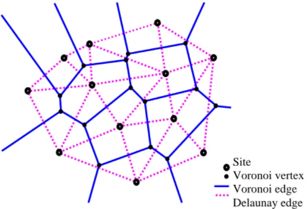
(2) 2. Related Work Coverage problems in sensor networks have been studied by many researchers. Meguerdichian and et al. [1] applied the computational geometry theory, Voronoi diagram and Delaunay triangulation, on the proposed coverage problems. They presented algorithms using computational geometry techniques to solve the coverage problems. Because the structures of Voronoi diagram and Delaunay triangulation are hard to be constructed efficiently in a distributed way, the algorithms they proposed were centralized algorithms. Li and et al. [2] proved the correctness of the above algorithms proposed in [1]. They also proved that there exist optimum best support paths in the Gabriel graph and the relative neighborhood graph of the sensor nodes. Hence, a distributed algorithm for finding a best support path is also proposed. In addition, Li and et al. [2] presented algorithms for finding best support paths with the least energy consumption and smallest total length. The topology of the sensor networks changes continuously over time, due to the instability of some sensors or the insertion of new sensors. Huang and Richa [3] studied the problem of how to dynamically maintain the measures of the best-case coverage and worst-case coverage distance. Their algorithms maintain a (1+ ε )-approximation on the best-case coverage distance and a ( 2 + ε ) -approximation on the worst-case coverage distance of the network, for any givenε> 0. Meguerdichian and et al. [4] proposed an exposure-based formulation analyzing the coverage of paths in a sensor network. The exposure is an integral measure of how well the sensor network can observe on a path over a period of time. A solution for finding minimal exposure path is developed in this work. They formally define exposure and study its properties, and then develop an algorithm for exposure calculations in sensor networks for finding minimal exposure path.. Assume a sensor network be represented by a set of n sites, S, in a two-dimensional field (or plane). A partition of the plane is created by assigning every point on the plane to its nearest site. All points assigned to a same site, p, form the Voronoi region, V(p), which is always convex. The edges shared by two Voronoi regions are called Voronoi edges and the end points of a Voronoi edge are called Voronoi vertices. Voronoi edges and Voronoi vertices form the Voronoi diagram, V(S), of a sensor network, S. A distinct property of Voronoi diagram is that a Voronoi edge must be associated with two nearest sites and a Voronoi vertex must be associated with at least three nearest sites. In addition, we assume that there exist no four sites of S that are co-circular, and every Voronoi vertex is exactly of degree three. The Delaunay triangulation of the network S, denoted as D(S), is the dual structure of a Voronoi diagram, which is constructed by connecting the sites in S whose Voronoi regions are next to each other. The boundary of D(S) forms a convex hull 1 of the sites. Figure 2 illustrates the properties described here, where the Voronoi diagram is plotted in solid lines and Delaunay triangulation in dash lines.. Site Voronoi vertex Voronoi edge Delaunay edge. Figure 2. The Voronoi Diagram and the Delaunay triangulation of a set of sites in a two-dimensional plane.. 3. Preliminaries 3.1 Sensor Network Model In this paper, we assume that sensors are deployed inside a square area of the two-dimensional field and belonged to an isotropic class. All sensors have identical sensitivity and their ability to sense a phenomenon decreases as the distance between a sensor and the phenomenon increases. Furthermore, we assume that the locations of all the sensors are known which can be found by either Global Positioning System (GPS), or any other location discovery techniques as described in [5].. 3.2 Computational Geometry Since Voronoi diagram and Delaunay triangulation [6, 7, 8] will be utilized in this paper, we need to describe some related computational geometry below.. 3.3 Problem Formulation We first introduce the notations that will be used for developing the proposed solution. The sensors are deployed in a two-dimensional field and they are represented as a set, S, of n sites. Let |xy| denote the Euclidean distance between the two sensors nodes, x and y. The distance of a point, x, to a set of points, V, denoted as dist(x, V), defines the smallest distance from x to any point in V. Given two point sets, U and V, the distance between U and V, dist(U, V), is defined as minxœU,yœV|xy| and the support-distance of U by V, support(U, V), is defined as max xœU dist(x,V). Figures 3 illustrate the definition of dist(x, V) and support(U, V), respectively. 1. - 600 -. The smallest convex polygon enclosing the network S..

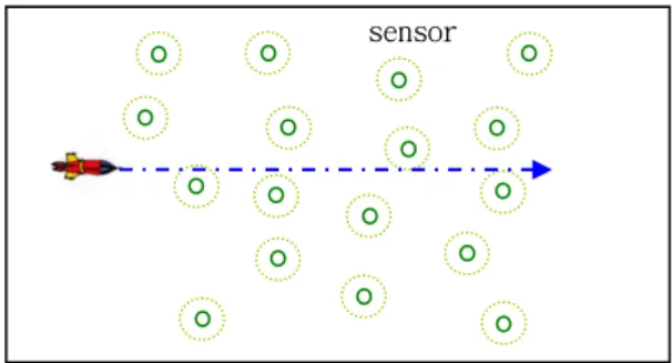
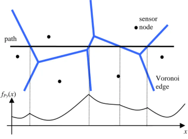
(3) Given a line path, P, the support of P is defined as support(P, S) which specifies the smallest observability of the points on the path, and the breach of P is defined as dist(P, S) which specifies the biggest obervability of the points on the path. In this paper, we assume that the sensors are deployed inside a square area whose boundary is parallel to x or y axis. Let (Xleft, Ytop) denote the left-top point of the square area, and (Xright, Ybot) denote the button-right point of the square area. For convenience, the line paths are assumed to be parallel to x axis and denoted as Py, where y specifies its y coordinate. We also assume the path starts at Xleft and ends at Xright. For a wireless sensor network, the best support line path and maximal breach line path are defined as follows: Definition: Best Support Line Path. A line path P that has the minimum support, support(P, S), is called a best support line path.. function, the maximal value always occurs at the intersection of the path and some Voronoi edge, as shown in Lemma 1 bellow. Lemma 1. Given a line path and a set of sensor nodes, the point on the path which has the maximal distance (support) to the sensors locates on either the end points of the path or the intersection of some Voronoi edge and the line path. Proof. The line path crosses the Voronoi diagram, and it is cut into several sub-paths as shown in Fighre 4. Each sub-path is inside a Voronoi region. Therefore, the distance function of this sub-path is also a part of hyperbolic curve. Because of the convexity of the distance function, the maximal value happens at one of the end of the sub-path. Hence, the overall maximal value will occur at the end points of the path or the intersection of some Voronoi edge and the path.. Definition: Maximal Breach Line Path. A Line path P that has the maximum breach, dist(P, S), is called a maximal breach line path.. sensor node. Thus, the line coverage problem for wireless sensor networks is to identify the best support line path and the maximal breach line path in the networks.. path. Voronoi edge. x dist. U. V v. fPy(x). u. x. u. support. V v. x. y Figure 4: Distance function of a line path.. Figure 3. An illustration of dist(x, V) and support(U, V). 4.2 Algorithm for Worst-case line coverage. Before we propose our algorithms, we will first discuss some important properties between the line path and the sensor network.. The breach of a line path is equal to the minimal value of the distance function of the path, and the maximal breach line path is the path whose distance function has the maximal minimal value. Therefore we have the algorithm for worst-case line coverage as described below.. 4.1 Distance function of a line path. Maximal Breach Line Path Algorithm. Given a line path, Py, and the sensor network, S, the distance function of Py describes the distance from the path to the network. Let fPy(x) denote the distance function of Py, and by the definition of section 3, fPy(x) = dist ((x,y), S), where x is in the interval [Xleft, Xright]. If there is only one sensor in the network, the distance function will be a half part of hyperbolic curve. In this case, let (x0, y0) be the coordinate of the sensor node. Then, fPy(x)=dist((x,y),(x0,y0))= ( x − x 0 ) 2 + ( y − y 0 ) 2 ,. 1. Sort the sensor nodes according to their y coordinates, and let the result be s1, …, sn. 2. Find the pair (si, si+1) whose difference of y coordinates is maximal, and let yi and yi+1 be the y coordinates of si and si+1, respectively. 3. The y coordinate of the maximal breach line path is (yi+yi+1)/2.. 4. Worst-case line coverage. which is a hyperbolic curve. According to the definition of breach and support, breach(Py) is equal to the minimal value of the distance function, fPy(x), and support(Py) is equal to the maximal value of fPy(x). Due to the convexity of the distance. 5. Best-case line coverage The best-case line problem is to find the horizontal path whose support is minimal. Therefore, all possible x and y coordinate values between inside the sensor field must be evaluated. Fortunately, by Lemma 1, the. - 601 -.

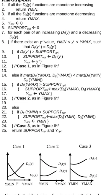
(4) support of a horizontal path happens at the intersection of the path and Voronoi edges. Thus, it doesn’t need to evaluate every x coordinate. This section describes the algorithm finding the best support line path.. 5.1 Best support line path algorithm We develop a plane sweep algorithm to solve the best-case line coverage problem. In the proposed algorithm, the sensor field is first partitioned into non-overlapped horizontal strips. The optimal y coordinate in every strip is then computed from the bottom strip to the top strip. The algorithm is described bellow. Best Support Line Path Algorithm 1. Partition the sensor field into horizontal strips using horizontal lines that pass the Voronoi vertices and the orthogonal intersections of Voronoi edges and Delaunay edges. (as shown in Figure 5) 2. From the bottom strip to the top strip, use Find-Strip-Best algorithm to find the optimal y coordinate in the strip and update the global optimal y coordinate of the line path.. Find-Strip-Best 1. 2. 3. 4. 5. 6. 7.. if all the Dli(y) functions are monotone increasing return YMIN. if all the Dli(y) functions are monotone decreasing return YMAX. Yopt Å 0 SUPPORTopt Å 0 for each pair of an increasing Dli(y) and a decreasing Dlj(y) 8. { if there exist an y′ value, YMIN < y′ < YMAX, such that Dli(y′ ) = Dlj(y′) 9. { if Dli(y′ ) > SUPPORTopt { SUPPORTopt Å Dli (y′) 10. 11. Yopt Å y′ } 12. } /*Case 1, as in Figure 6*/ 13. 14. else if max(Dli(YMAX), Dlj(YMAX)) < max(Dli(YMIN), Dlj (YMIN)) 15. { if Dli(YMAX) > SUPPORTopt 16. { SUPPORToptÅmax(Dli(YMAX), Dlj(YMAX)) 17. Yopt Å YMAX } 18. } /*Case 2, as in Figure 6*/ 19. 20. else 21. { if Dli (YMIN) > SUPPORTopt 22. { SUPPORToptÅmax(Dli(YMIN), Dlj(YMIN)) Yopt Å YMIN } 23. 24. } /*Case 3, as in Figure 6*/ 25. return SUPPORTopt and Yopt. Case 1. Case 3. Case 2. strip Dli(y) Dli(y). Dlj(y) Dli(y). Dlj(y) Delaunay edge. YMIN y′ YMAX. Voronoi edge. Dlj(y) YMIN. YMAX YMIN. YMAX. Figure 6. An illustration of an increasing Dli (y) and a decreasing Dlj (y). Figure 5. The sensor field is partitioned into strips. In the first step of the algorithm, Voronoi edges are cut into segments by the strips. For a given strip, we assume that there are m Voronoi edge segments in this strip, and let the segments be l1, …, lm. If there is a horizontal path, Py, in this strip, the maximal value of its distance function occurs at the intersection of the path and those segments. Let Dli(y) be the distance from the intersection of li and Py to the sensors. Because the cutting points of the strips are Voronoi vertices and orthogonal intersections of Voronoi edges and Delaunay edges , Dli(y) is either monotone increasing or monotone decreasing with respect to y. Let YMIN and YMAX be the bottom and top y coordinate of the strip. If all the Dli(y) functions are increasing, the optimal y coordinate is equal to YMIN. On the other hand, if all the Dli(y) functions are decreasing, the optimal y coordinate is equal to YMAX. The Find-Strip-Best algorithm finds the optimal y coordinate of a strip as describe bellow.. Lemma 2. Inside a strip, as a line path with the Yopt coordinate found by Find-Strip-Best algorithm crosses the Voronoi edges, the distance values of the intersections of the path and Voronoi edges are smaller than or equal to the support value, SUPPORTopt, found by Find-Strip-Best. Proof. Assume the Yopt found by the algorithm is achieved by Dli(y) and Dlj(y) of case 1. The proofs of other cases are similar and are omitted here. Suppose there exist a segment lk, and Dlk (Yopt) > SUPPORTopt = Dli (Yopt) = Dlj (Yopt). If Dlk (y) is monotone increasing, we can find a y′ coordinate, y′ < Yopt, such that Dlk(y′) = Dlj (y′) > SUPPORTopt, as shown in Figure 7(a). On the other hand, if Dlk (y) is monotone decreasing, we can find a y′ coordinate, y′> Yopt, such that Dlk(y′) = Dli (y′) > SUPPORTopt, as shown in Figure. - 602 -.

(5) 7(b). Due to this contradiction, the lemma follows.. 7. Conclusion Based on Lemma 2, we can proof the correctness of Find-Strip-Best algorithm. Theorem 1. Given a strip, the Yopt coordinate found by Find-Strip-Best algorithm is the optimal y coordinate and the support of the path, PYopt, is minimal in the strip. Proof. Assume Yopt found by the algorithm is achieved by Dli(y) and Dlj(y) of case 1. By Lemma 2, for any other segment lk, Dlk (Yopt) ≦ Dli (Yopt) = Dlj (Yopt) = SUPPORTopt. Therefore, SUPPORTopt is the support value for PYopt. If y′ ≠ Yopt and YMIN < y′ < YMAX, either Dli (y′) or Dlj(y′) is larger than SUPPORTopt. Thus, the support of Py′ is larger than that of Yopt. The proofs of other cases are similar and are omitted. (a). (b). Dlk(y) Dli(y). Dli(y). Dlk(y) Dlj(y). References. Dlj(y). y′ Yopt. Yopt. y′. Figure 7. An illustration of Lemma 2.. 6. Experimental Results We evaluate the proposed best support line coverage algorithm and compare it with a grid method. In our experiments, the sensors are randomly deployed into a 100x100 m2 square area. The numbers of sensor nodes are from 50 to 250. In the grid method, the square area is divided into 1000x1000 grids, and the support value is then calculated approximately on the grid points. Figure 8 shows the result of experiment. From the result, the proposed optimal algorithm outperforms the grid method. Experiment Result 15 Support(m). In this paper, we present the formulations for best-case and worst-case line coverage problems in wireless sensor networks. Optimal polynomial time algorithms using graph theory and computational geometry are proposed to solve the problems. The distance function of a line path is introduced. With the distance function, the support and breach correspond to the maximal and minimal values of the function. Furthermore, we prove that the maximal value of the distance function always occurs at some intersection of Voronoi edges and the path. Base on that, a plane sweep algorithm is proposed to solve the best-case line coverage problem. Other interesting coverage problems may be investigated in the future, such as finding the maximal breach path and best support path in a three-dimensional space. Due to the unreliability of sensor nodes, finding best coverage path over the sensor networks might also be useful in military applications.. 10. Grid Our algorithm. 5. [1] S. Meguerdichian, F. Koushanfar, M. Potkonjak, and M. Srivastava “Coverage Problems in Wireless Ad-Hoc Sensor Network,” Proc. IEEE INFOCOM ’01, pp. 1380-1378, 2001. [2] X.-Y. Li, P.-J. Wan, O. Frieder “Coverage in Wireless Ad-Hoc Sensor Networks,” Proc. IEEE Trans. Computers, vol.52, no. 6, JUNE 2003. [3] H. Huang and A.W. Richa, “Dynamic Coverage in Ad-Hoc Sensor Networks,” Mobile Networks and Applications 10, 9-17, 2005. [4] S. Meguerdichian, F. Koushanfar, G Qu, and M. Potkonjak “Exposure in Wireless Ad-Hoc Sensor Networks,” Proc. of 7th Annual International Conference on Mobile Computing and Networking (MobiCom’01), pp. 139-150, July 2001. [5] A. Savvides, C.C. Han, and M.B. Srivastava, “Dynamic Fine-Grained Localization in Ad Hoc Networks of Sensors,” Proc. Seventh Ann. Int’l Conf. Mobile Computing and Networking (Mobi-COM 2001), July 2001. [6] S. Fortune, “Voronoi Diagrams and Delaunay Triangulations,” Computing in Euclidean Geometry, F.K. Hwang and D.-Z. Du, eds., pp. 193-233, Singapore: World Scientific, 1992. [7] J. O’Rourke, Combinatorial Geometry in C. Cambridge, 1998. [8] F.P. Preparata and M.I. Shamos, Computational Geometry: AnIntroduction. Springer-Verlag, 1985. [9] T.J. Cormen, C.E. Leiserson, and R.L. Rivst, Introduction to Algorithms. MIT Press and McGraw-Hill, 1990.. 0 50. 100. 150. 200. 250. Sensor nodes. Figure 8. The support find by the proposed algorithm and grid method.. - 603 -.

(6)