行政院國家科學委員會專題研究計畫 成果報告
美國最低稅負制度對捐贈行為之影響
計畫類別: 個別型計畫 計畫編號: NSC95-2415-H-004-001- 執行期間: 95 年 01 月 01 日至 95 年 07 月 31 日 執行單位: 國立政治大學財政系 計畫主持人: 羅光達 報告類型: 精簡報告 處理方式: 本計畫可公開查詢中 華 民 國 95 年 10 月 17 日
中文摘要
美國最低稅負制度的實施是希望高所得者過度利用稅法上給予之租稅優 惠,進而規避或甚至免繳任何租稅之不合理現象能有所改善。其實施之要點在於 將高所得者常利用的租稅優惠減免重新納入其所得基礎,再根據新的規定計算其 應繳納之最低稅額。根據統計,美國高所得者就常利用所得稅法上對非現金捐贈 扣除額的優惠,進行租稅規避。為矯正此一現象,美國在 1986 年的稅法修正法 案(TRA86)中,特別在最低稅負稅法上規定,個人非現金捐贈只能以其成本做 為扣除額之上限,而不再是以公平市價做為減免基礎。相較於一般所得稅法之規 定,此一扣除額之限制,將造成個人非現金捐贈租稅價格的提高。 本研究計畫之目的即在於希望能針對上述美國最低稅負制度對非現金捐贈 扣除額之限制規定,利用差異中之差異估計法(Difference-in-Difference Approach)來衡量捐贈行為之租稅效果。研究結果顯示,TRA86 對非現金扣除額 的上限規定將使得納稅人減少其慈善捐贈,惟此一效果並不顯著。Abstract
This project attempts to investigate how and to what extent the alternative minimum tax (AMT) affects individuals’ charitable contributions. The Tax Reform Act 1986 included a provision that limited the AMT taxpayer’s deduction for the charitable contribution of appreciated property only to the adjusted cost basis in the property. This regulation increases the tax price of appreciated property gifts. In this study we try to identify the impacts of AMT regulations on charitable contributions with the help of the difference-in-difference (DID) approach. The results from our DID estimations indicate that the TRA86 has a negative impact on charitable contributions, though its effect is not significant.
Keywords: charitable contributions, difference-in-difference estimation. JEL classification: C31, H24, H31.
Introduction
Economists have long paid attention to contribution behaviors because most households donate charitable contributions in any given year. Nearly 90% of households in U.S. made charitable contributions, and the average contributing household gave $1,620, or 3.2% of household income. In addition, private
philanthropy in the US is also a major industry, amounting to $212 billion in 20011. Contributions include of cash and non-cash gifts, which may be property, stocks and other items of value. The Federal and state governments subsidize this activity by allowing the amount of charitable contributions to approved charities to be deducted from taxable income by itemizing taxpayers. Further, tax laws permit taxpayers who donate appreciated property to take a full deduction for the fair market value of property without paying capital gains tax on the appreciated component. Together, these two provisions of the tax law significantly lower the “price” of charitable contributions to the taxpayer.
Understanding how the tax system affects the level of charitable giving overall and by taxpayers in different income groups is a major research area that is of interest to policy-makers and research scholars alike. The revenue cost of the charitable gifts deduction to the Federal government alone was $28 billion in 20012, and much of this tax reduction accrued to high income taxpayers. Philanthropic organizations labor mightily to retain this tax preference, arguing that it increases charitable giving significantly. Although most people make donations each year, the bulk of the donations come from the rich. Households in the top four percent of the income distribution gave over 40 percent of the charitable contributions in 1995 (Havens and Schervish, 1999). In many cases, wealthy people donate appreciated property in order to take advantage of double tax benefits. Such donors receive a deduction for the asset’s current market fair value and avoid paying tax on the capital gains that would otherwise have been due upon the sale of the asset. For this reason, much of the research on this topic focuses on charitable giving by high income taxpayers, as will the research proposed here.
Typically, research into the effects of the tax system on charitable gifts focuses
1
on how the tax system affects the price of charitable giving. For example, an
itemizing taxpayer in the 28% tax bracket faces a net price of 72 cents for a one dollar gift. A taxpayer in a higher tax bracket faces a lower price, and a taxpayer in the highest bracket making a gift of appreciated property faces the lowest price of all. The price of a dollar gift consisting mostly of appreciated property could be as little as 40 cents to such a taxpayer.
Many researchers use the variation in the price of charity to taxpayers in different brackets as a means of estimating the impact of the tax system on the level of giving. Such an approach suffers from what an econometrician would call an “identification” problem. Higher income is likely to affect the level of giving, as well as the price of giving. Hence the effect of price and the effect of income are entangled, because the level of a taxpayer’s income determines his or her tax bracket. Any
estimate of the effect of the tax system on giving through its effect on price would be seriously biased using this methodology.
Some researchers have tried to solve the identification problem by focusing on changes in tax rates that occur over time. Such research poses the problem of untangling other events that might affect charitable giving, including changes in income, which occur over the same time interval as the change in tax rates. A more promising line of research uses difference in state income tax rates as a means of identifying the impact of price on giving (Feenberg, 1987).
We here propose another method of identifying the impact of the tax system on the level of giving. Rich taxpayers not only account for much of charitable giving, they are also a group most likely to be affected by the Alternative Minimum Tax (AMT). The AMT is a separate system of income taxation that operates in parallel to the regular income tax system, but with different rules and different tax rates. In 2000, 1.3 million taxpayers were subject to the AMT. The goal of the AMT for individuals is to ensure that everyone with significant income pays sufficient federal income tax. The AMT has a lower top rate than the regular income tax but tries to capture more income by defining taxable income more broadly. Compared to the regular income tax, the AMT has fewer “tax preferences” (deductions) and other ways of reducing tax liability. In other words, the AMT is devised to reduce the amounts of deductions
2
used more frequently by high-income taxpayers and infrequently by others.
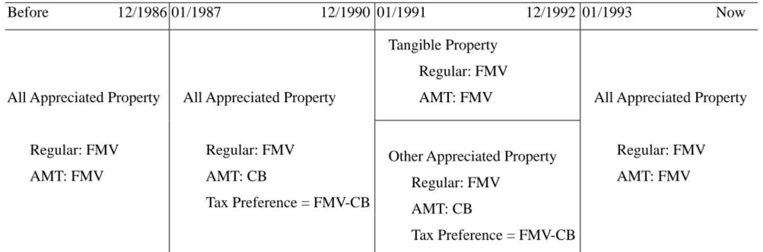
The charitable contributions deduction is one such deduction, and for a period of time between 1986 and 1993, taxpayers subject to the AMT faced different charitable contribution deduction rules from taxpayers filing under the regular system. Prior to 1986, both AMT and non-AMT taxpayers received a full deduction under the Federal personal income tax for the fair market value of appreciated property. After 1986, there were major changes in the treatment of appreciated property donations under the AMT. The Tax Reform Act 1986 included a provision that limited a taxpayer’s deduction for the charitable contribution of appreciated property to the adjusted cost basis in the property. The Omnibus Budget Reconciliation Act of 1990 repealed this provision for tangible personal property, and the 1993 Act repealed the provision for all other appreciated property classes, thus restoring the pre-1986 rules (but not the tax rates). Table 1 shows the different tax treatments under regular income tax and the AMT during different periods.
Table 1: The Allowable Deduction Amounts of Appreciate Property Contributions
Before 12/1986 01/1987 12/1990 01/1991 12/1992 01/1993 Now Tangible Property
Regular: FMV AMT: FMV All Appreciated Property
Regular: FMV AMT: FMV
All Appreciated Property
Regular: FMV AMT: CB
Tax Preference = FMV-CB
Other Appreciated Property Regular: FMV
AMT: CB
Tax Preference = FMV-CB
All Appreciated Property
Regular: FMV AMT: FMV
Notes: FMV: Fair Market Value; CB: Cost Basis.
We propose to use the varying treatment of appreciated property under the AMT as a means of identifying the impact of the tax system on giving through its effect on the price of charity.
Methodology
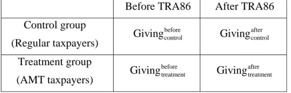
AMT taxpayers experienced different tax treatments for appreciated gifts in different periods while the regular taxpayers did not; therefore, in this research, we use the difference-in-difference (DID) approach to identify how and to what extent the alternative minimum tax affects individuals’ charitable contributions. This method is similar to the treatment effect concept, in which one group has been exposed to some sort of catalyst or has experienced some policy change (treatment group) while the other group has not (control group). Thus, we here define the control group comprises the regular taxpayers and the treatment group is composed of the AMT taxpayers. In addition, we use The Tax Reform Act 1986 (TRA86) as our new tax policy, in which included a provision that limited a taxpayer’s deduction for the charitable contribution of appreciated property to the adjusted cost basis in the property. Usually a
difference-in-difference approach is utilized to examine the effects of a natural experiment on two different groups. The major feature of this estimation approach is we can control for nontax effects that coincide with tax reforms. We can use Table 2 to explain our identification strategy.
Table 2: Control Group and Treatment Group
Before TRA86 After TRA86
Control group (Regular taxpayers)
before control
Giving Givingaftercontrol
Treatment group (AMT taxpayers)
before treatment
Giving Givingaftertreatment
The change in giving of our treatment group is ( ).
This change comes from an increase in the tax price of giving and some nontax factors (e.g., change in economic environment or in social norms). A critical
assumption in the difference-in-difference approach is that the changes in the nontax factors have the same effects on the control group and the treatment group. Thus, the nontax factor effects on the treatment group are also reflected in the change in giving
for the control group, which is ( ). If we compare the change
after before treatment treatment Giving −Giving after before control control Giving −Giving
in giving for the treatment group with the change in giving for control group, then the difference can be used as an indicator of how the tax policy affects individuals’ giving decisions. As Triest (1998) argues, by using difference-in-difference estimation, we can isolate the nontax effects first, by identifying the change in the behavior before and after a natural experiment, and then obtain the pure effect of taxation on individuals’ behaviors from a comparison of the changes in control and treatment groups. In other words, the difference-in-difference estimate representing the pure tax effect can be described in the following equation:
DID estimate = (Givingaftertreatment −Givingbeforetreatment) (Giving− aftercontrol−Givingbeforecontrol)……(1) From equation (1), the difference-in-difference regression specification used in this study to estimate the impact of the change in the tax price on charitable
contributions is described as follows:
∑
+ + × + + +=α αTreatment α After α After Treatment Xβ ε
Giving) ( )
ln( 0 1 2 3 …(2)
Here Giving indicates charitable contributions3. is a dummy variable that equals 1 for the treatment group and 0 for the control group.
Treatment
After is a
time dummy that is 1 for the year after 1986 and 0 for the year before 1986. is a set of control variables including income, wealth, age, martial status and number of dependents.
X
ε is the error term. It is worth noting that the price of giving does not enter our estimation directly. Instead, we use a policy change (i.e., tax price of giving increased for the treatment group only) to estimate the price effect indirectly. This feature allows us to avoid the identification problem existing in conventional estimations in previous studies.
In equation (2), the difference in giving for the treatment group before and after the policy change is α α2+ , and the difference in giving for the control group before 3 and after the policy change is α2. Therefore, α3, the difference-in-difference
estimator, can be considered the pure tax effect for the treatment group before and after the policy changes.
3
Charitable contributions could be cash giving only, noncash giving only, and total giving (cash giving and noncash giving).
Data and Variables
The data set employed for this study is 1985 and 1987 Individual Tax Model File (IMF) panel data from the Internal Revenue Service, maintained by the Office of Tax Policy Research at the University of Michigan. The measurement of each variable we need in the estimation is described below.
Giving: Cash giving and noncash giving (appreciated giving) are the amounts of
taxpayers’ reported charitable deductions on their tax returns. The total giving is the sum of these two types of contributions. We keep the individuals who have zero cash giving or zero noncash giving in our sample4. To avoid taking the log of zero, we follow the conventional practice adding $10 in taxpayers’ reported giving amounts.
Income: The basic income measure used in previous literature is first-dollar
disposable income, which is calculated here as adjusted gross income (AGI) plus IRA and Keogh plan contributions less the amount of tax liability had no charitable
contrition been made. To avoid taking the logarithm of zero or a negative value, only taxpayers with positive income were included in the sample.
Other explanatory variables: In addition to income and the dummy variables of
After, Treatment and the interaction term of after and treatment (After*Treatment), some variables available on tax returns data are also important determinants on charitable contributions. Here the X vector includes wealth measure5, age6, marital status, and the number of dependents. We expect individuals with larger amount of wealth within any income level to make larger donations, ceteris paribus, thus the estimate of this variable should be positive. Age has been used and consistently found to be an important factor in explaining differences in personal giving propensities. Besides, researchers also believe that unmarried taxpayers have a different perspective about charitable contributions than do married taxpayers. All previous studies have
4
Because some individuals may have zero contributions, the Tobit model was applied here to eliminate the censoring bias.
5
O’Neil et al. (1996) mentioned that direct measures of wealth are never available from tax returns data; therefore, we follow their method using gross interest income and dividend income as an indirect measure of wealth. Again, to avoid taking the logarithm of zero or a negative value, only taxpayers with positive wealth were included in the sample.
6
found that married individuals make larger donations, ceteris paribus. As O’Neil et al (1996) stated, the presence of dependents may have either a positive or a negative influence on the amount of giving. With more dependents, the income per individual in the household unit decreases, ceteris paribus, thus it might be expected that contributions would decline. However, families with dependents are more likely to participate in some church and education nonprofit organizations, leading to higher giving.
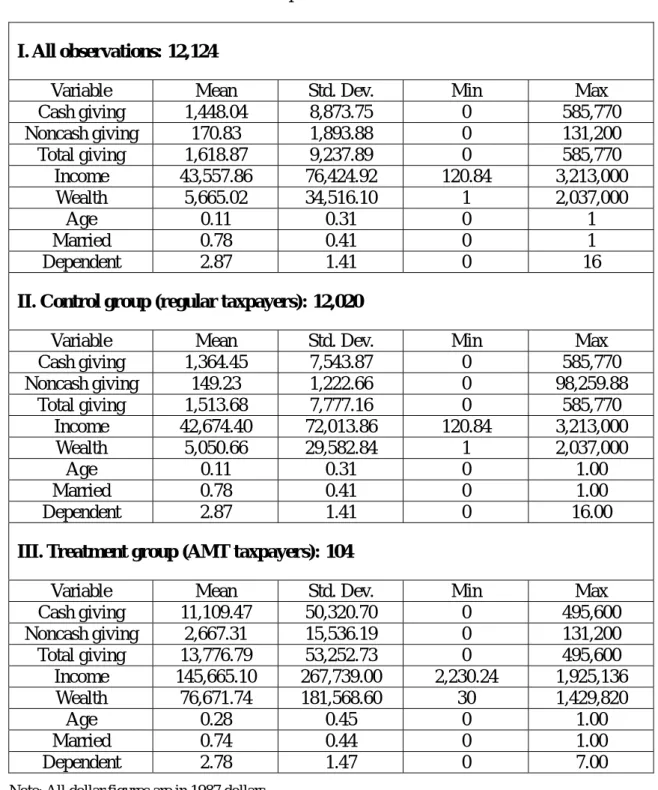
After the data management, we have 12,124 observations in the sample, where there are 6,256 (5,764) individuals in the control group and 77 (27) in the treatment group in 1985 (1987). The sample statistics are presented in Table 3. Some
differences are evident between the treatment group and the control group. Measured according to mean values, the treatment group gave more charitable contributions than the control group. Additionally, the treatment group has more income and wealth but claims fewer dependents. A higher percentage of taxpayers in the treatment group are aged 65 or over. Besides, a lower percentage of the treatment group is married.
Table 3: Descriptive Statistics of Variables
I. All observations: 12,124
Variable Mean Std. Dev. Min Max
Cash giving 1,448.04 8,873.75 0 585,770 Noncash giving 170.83 1,893.88 0 131,200 Total giving 1,618.87 9,237.89 0 585,770 Income 43,557.86 76,424.92 120.84 3,213,000 Wealth 5,665.02 34,516.10 1 2,037,000 Age 0.11 0.31 0 1 Married 0.78 0.41 0 1 Dependent 2.87 1.41 0 16
II. Control group (regular taxpayers): 12,020
Variable Mean Std. Dev. Min Max
Cash giving 1,364.45 7,543.87 0 585,770 Noncash giving 149.23 1,222.66 0 98,259.88 Total giving 1,513.68 7,777.16 0 585,770 Income 42,674.40 72,013.86 120.84 3,213,000 Wealth 5,050.66 29,582.84 1 2,037,000 Age 0.11 0.31 0 1.00 Married 0.78 0.41 0 1.00 Dependent 2.87 1.41 0 16.00
III. Treatment group (AMT taxpayers): 104
Variable Mean Std. Dev. Min Max
Cash giving 11,109.47 50,320.70 0 495,600 Noncash giving 2,667.31 15,536.19 0 131,200 Total giving 13,776.79 53,252.73 0 495,600 Income 145,665.10 267,739.00 2,230.24 1,925,136 Wealth 76,671.74 181,568.60 30 1,429,820 Age 0.28 0.45 0 1.00 Married 0.74 0.44 0 1.00 Dependent 2.78 1.47 0 7.00
Results and Discussions
In Table 4, we estimate how the Tax Reform Act 1986 (TRA86) affects the AMT taxpayers’ noncash giving, in which. TRA86 included a provision that limited a taxpayer’s deduction for the charitable contribution of appreciated property to the adjusted cost basis in the property. As previous studies demonstrate, income and wealth are still positive determinants of noncash contributions. People who are aged 65 or above, married and have more dependents are more likely to contribute more than people with the opposite characteristics.
Our key variable is , which is the difference-in-difference estimator representing the policy effect. The coefficient of this variable is –0.555. This result tells us that, if the policy were implemented to limit a taxpayer’s deduction for the noncash giving to the adjusted cost basis, then the treatment group (AMT taxpayers), ceteris paribus, would decrease their noncash giving, though the effects would not be statistically significant.
Treatment After×
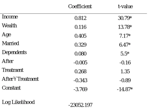
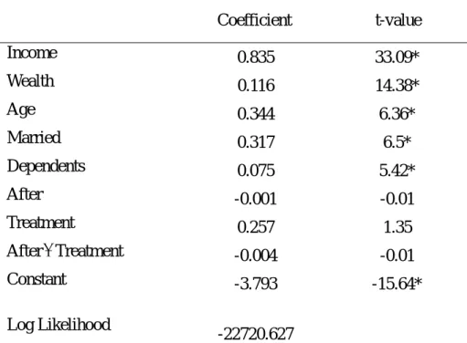
Table 5 and Table 6 shows the empirical results when the dependent variables are cash giving and total giving, respectively. Like the results in Table 4, income, wealth and other demographic variables have the same expected signs. Unfortunately, the coefficient of After×Treatment is still insignificantly negative.
From our results we know that, if the government only allows taxpayers to deduct their charitable contributions of appreciated property to the adjusted cost basis, not to the full market value like cash giving, taxpayers will decrease their charitable contribution; however, the effect is not significant. The reason of
insignificance can be attributed to the too few observations in the treatment group. In fact, we only obtained 104 AMT taxpayers in our sample, compared to 12,020 observations in the control group.
Conclusions and Future Work
Identifying the true tax price effect on charitable contributions is hindered by the facts that we do not have too much variation in tax prices under the current tax system, and we are not able to know the accurate functional form of tax rates and other factors, such as incomes, in advance. In previous studies, authors have tried to find some sources of variation in tax rates that are independent of individuals’ incomes to
improve the estimation results. However, unless we have considerable confidence that all individual variation in tax prices correlated with incomes has been removed, the estimates of price effects may still include part of income effects. In order to solve this identification problem, we here employ a difference-in-difference approach, using an exogenous change in tax rates from a natural experiment, to estimate the tax price effect on charitable contributions.
The results from our difference-in-difference estimation, allowing us to avoid the identification problem existing in previous studies, indicate that the TRA86 has a negative impact on charitable contributions, though its effect is not significant. Because we are not able to obtain large enough observations in the treatment group from the IMF pane data, we here suggest that the future research can use the IMF cross section data for this study7.
7
The size of random sample for each cross section individual year in IMF data varies from year to year, between 80,000 to 250,000 tax returns.
Table 4: Difference-in-Difference Estimates for Noncash Giving Coefficient t-value Income 1.251 15.43* Wealth 0.118 4.7* Age 0.451 2.65* Married 0.379 2.5* Dependents 0.060 4.43* After 0.058 0.62 Treatment -0.573 -1 After Treatment × -0.555 -0.52 Constant -13.916 -17.59* Log Likelihood -14315.893
Note: * indicates significance at the 95% level. The t-statistics are in parentheses.
Table 5: Difference-in-Difference Estimates for Cash Giving
Coefficient t-value Income 0.812 30.79* Wealth 0.116 13.78* Age 0.405 7.17* Married 0.329 6.47* Dependents 0.080 5.5* After -0.005 -0.16 Treatment 0.268 1.35 After Treatment × -0.343 -0.89 Constant -3.769 -14.87* Log Likelihood -23052.197
Table 6: Difference-in-Difference Estimates for Total Giving Coefficient t-value Income 0.835 33.09* Wealth 0.116 14.38* Age 0.344 6.36* Married 0.317 6.5* Dependents 0.075 5.42* After -0.001 -0.01 Treatment 0.257 1.35 After Treatment × -0.004 -0.01 Constant -3.793 -15.64* Log Likelihood -22720.627
References
Feenberg, Daniel (1987), “Are Tax Price Models Really Identified: The Case of Charitable Giving”, National Tax Journal, 40(4), 629-633.
O’Neil, Cherie J., Richard Steinberg, G. and Rodney Thompson (1996), “Reassessing the Tax-Favored Status of the Charitable Deduction for Gifts of Appreciated Assets”, National Tax Journal, 49(2), 215-233.
Triest, Robert K. (1998), “Econometric Issues in Estimating the Behavioral Response to Taxation: A Nontechnical Introduction”, National Tax Journal, 51(4), 761-772.