馬可夫鏈蒙地卡羅收斂的研究與貝氏漸進的表現 - 政大學術集成

全文

(1)國立政治大學統計學系博士學位論文指導教授: 翁久幸博士. 政治大馬可夫鏈蒙地卡羅收斂的研究與貝氏漸進的表現立. ‧ 國. 學 ‧. A Study of MCMC Convergence and Performance sit. y. Nat. n. al. er. io. Evaluation of Bayesian Asymptotics Ch. engchi. i Un. v. 研究生: 許正宏撰中華民國一百年六月.

(2) 謝辭本論文能順利完成, 幸蒙吾師翁久幸教授的悉心指導, 舉凡研究方向, 觀念的啟迪, 架構的匡正, 求學態度的斧正, 乃至於本論文內容的逐字批閱與修飾, 特此獻上最深的敬意與感謝。同時, 也謝謝口試委員曹振海老師、蕭朱杏老師、徐南蓉老師、蔡紋琦老師與黃子銘老師於論文口試期間, 對我的鼓勵以及論文的指正, 遂使本論文得以臻於完備。修業期間, 感謝系上諸位老師在課業知識的傳授與助教在行政事務的協助。同時, 也謝謝同窗好友漢葳、金田、學弟宇翔、泰期、建郎的切磋討論與激勵, 獲益匪淺。隨著論文的付梓, 博士班的修業即將完成, 這段日子裏, 有挫折, 也有收穫和成長。經過這一段歷練, 不僅淬勵我的人生, 也讓自己的視野更宏觀。最後, 特別感謝我敬愛的雙親對我的養育與支持; 感謝內人慎如的包容與犧牲, 在她細心照顧小孩與操持家務下, 讓我能全心投入並順利完成論文。僅以本論文獻給我最摯愛的家人。. 立. 政治大. ‧. ‧ 國. 學. n. er. io. sit. y. Nat. al. Ch. n engchi U. 2. iv. 許正宏謹誌中華民國一百年六月.

(3) 中文摘要. 本論文主要討論貝氏漸近的比較, 推導出參數的聯合後驗分配與利用圖形來診斷馬可夫鏈蒙地卡羅的收斂。 Johnson (1970) 利用泰勒展開式得到個別後驗分配的展開式, 此展開式是根據概似函數與先驗分配。 Weng (2010b) 和 Weng and Hsu (2011) 利用 Stein’s 等式且由概似函數與先驗分配估計後驗動差; 將這些後驗動差代入 Edgeworth 展開式得到近似後驗分配, 此近似分配的誤差可精確到大 O 的負 3/2 次方與 Johnson’s 相同。另外 Weng and Hsu (2011) 發現 Weng (2010b) 和 Johnson (1970) 的近似展開式各別項誤差到大 O 的負 1 次方不一致, 由模擬結果得到 Weng’s 在此項表現比 Johnson’s 好。另外由 Weng (2010b) 得到一維參數的 Edgeworth 近似後驗分配延伸到二維參數的聯合後驗分配; 並應用二維參數的聯合後驗分配於多階段資料。本論文我們提出利用圖形來診斷馬可夫鏈蒙地卡羅收斂的方法, 並且應用一般化線性模型與混合常態模型做為模擬。. 立. 政治大. ‧. ‧ 國. 學. n. al. er. io. sit. y. Nat. 關鍵字: Edgeworth 展開式; 馬可夫鏈蒙地卡羅; 個別後驗分配; Stein’s 等式。. Ch. engchi. 3. i Un. v.

(4) Abstract Johnson (1970) obtained expansions for marginal posterior distributions through Taylor expansions. The expansion in Johnson (1970) is expressed in terms of the likelihood and the prior. Weng (2010b) and Weng and Hsu (2011) showed that by using Stein’s identity we can approximate the posterior moments in terms of the likelihood and the prior; then substituting these approximations into an Edgeworth series one can obtain an expansion which is correct to O(t−3/2 ), similar to Johnson’s. Weng and. 政治大 agree and further compared these two expansions by simulation study. The simulations 立 confirmed this finding and revealed that our O(t ) term gives better performance than Hsu (2011) found that the O(t−1 ) terms in Weng (2010b) and Johnson (1970) do not −1. ‧ 國. 學. Johnson’s. In addition to the comparison of Bayesian asymptotics, we try to extend Weng (2010a)’s Edgeworth series for the distribution of a single parameter to the joint. ‧. distribution of all parameters. Since the calculation is quite complicated, we only derive expansions for the two-parameter case and apply it to the experiment of multi-stage. sit. y. Nat. data. Markov Chain Monte Carlo (MCMC) is a popular method for making Bayesian inference. However, convergence of the chain is always an issue. Most of convergence. n. al. er. io. diagnosis in the literature is based solely on the simulation output. In this dissertation,. i Un. v. we proposed a graphical method for convergence diagnosis of the MCMC sequence. We. Ch. used some generalized linear models and mixture normal models for simulation study.. engchi. In summary, the goals of this dissertation are threefold: to compare some results in Bayesian asymptotics, to study the expansion for the joint distribution of the parameters and its applications, and to propose a method for convergence diagnosis of the MCMC sequence.. Key words:. Edgeworth expansion; Markov Chain Monte Carlo; marginal posterior. distribution; Stein’s identity..

(5) Contents 1 Introduction. 1. 2 Preliminaries. 3. 2.1. The Model. . . . . . . . . . . . . . . . . . . . . . . . . . . . . . . . . . . . .. 3. 2.2. Stein’s Identity and Bayesian Edgeworth Expansion . . . . . . . . . . . . .. 4. 2.3. The Laplace Method . . . . . . . . . . . . . . . . . . . . . . . . . . . . . . .. 7. 2.4. The Gibbs Sampling and MCMC Convergence Diagnostic . . . . . . . . . .. 8. 2.5. The Generalized Linear Model . . . . . . . . . . . . . . . . . . . . . . . . .. 9. 3 Theoretical Results. 10. 3.1. Validation of Simulation Results . . . . . . . . . . . . . . . . . . . . . . . .. 10. 3.2. Joint Posterior Distributions. 13. 立. . . . . . . . . . . . . . . . . . . . . . . . 政. . . 治大. 4 Experimental Results. 4.1.1. Comparison with Johnson (1970) . . . . . . . . . . . . . . . . . . . .. 20. 4.1.2. Comparison with Tierney and Kadane (1986) . . . . . . . . . . . . .. 25. Multi-stage Data . . . . . . . . . . . . . . . . . . . . . . . . . . . . . . . . .. 27. ‧ 國. y. Binomial Model . . . . . . . . . . . . . . . . . . . . . . . . . . . . . .. 4.2.2. Two-parameter Logit Model . . . . . . . . . . . . . . . . . . . . . . .. 29. er. 4.2.1. io. 28. sit. Nat. al. 29. 4.5. v Poisson Regression Model C h. . . . . . . . . .U. .n.i . . . . . . . . . . . . . . . Gamma Model . . . . . . .e. n . .g. c . .h. i. . . . . . . . . . . . . . . . . . . .. 4.6. Mixture Normal. 34. 4.4. Logit Model . . . . . . . . . . . . . . . . . . . . . . . . . . . . . . . . . . . .. n. 4.3. 20. ‧. 4.2. Comparison of Second Order Approximations . . . . . . . . . . . . . . . . .. 學. 4.1. 20. . . . . . . . . . . . . . . . . . . . . . . . . . . . . . . . . .. 5 Concluding Remarks. 32 33. 37. i.

(6) List of Figures Figure 1 Comparison with Johnson (1970) Beta-Binomial model . . . . . . . . . . . . . . . . . . . . . . 23 Figure 2 Comparison with Johnson (1970) Poisson-Gamma(30,5) . . . . . . . . . . . . . . . . . . . . . 24 Figure 3 Comparison with Johnson (1970) Poisson-Gamma(15,5) . . . . . . . . . . . . . . . . . . . . . 25 Figure 4 Comparison with Tierney and Kadane (1986) Logit2p-flat and N(0,1) . . . . . . . . 27 Figure 5 Comparison with Tierney and Kadane (1986) Probit3p-flat . . . . . . . . . . . . . . . . . . 27 Figure 6 Sequential update Beta-Binomial model . . . . . . . . . . . . . . . . . . . . . . . . . . . . . . . . . . . . . 46 Figure 7 Sequential update Logit model with joint posterior density prior . . . . . . . . . . . . . 46 Figure 8 Convergence diagnosis of MCMC: Logit2p-flat (small MCMC sample) . . . . . . . 47 Figure 9 Convergence diagnosis of MCMC: Logit2p-flat (large MCMC sample) . . . . . . . . 48 Figure 10 Convergence diagnosis of MCMC: Logit2p-N(0,1) . . . . . . . . . . . . . . . . . . . . . . . . . . . 49 Figure 11 Convergence diagnosis of MCMC: Logit3p-flat heavy tail . . . . . . . . . . . . . . . . . . . 50. 政治大 Figure 13 Convergence diagnosis 立 of MCMC: Logit3p-N(0,1) . . . . . . . . . . . . . . . . . . . . . . . . . . . 52 Figure 12 Convergence diagnosis of MCMC: Logit3p-flat . . . . . . . . . . . . . . . . . . . . . . . . . . . . . . 51. ‧ 國. 學. Figure 14 Convergence diagnosis of MCMC: Logit6p-flat . . . . . . . . . . . . . . . . . . . . . . . . . . . . . . 53 Figure 15 Convergence diagnosis of MCMC: Poisson2p-flat. . . . . . . . . . . . . . . . . . . . . . . . . . . .54 Figure 16 Convergence diagnosis of MCMC: Poisson2p-N(0,1) . . . . . . . . . . . . . . . . . . . . . . . . 55. ‧. Figure 17 Convergence diagnosis of MCMC: Gamma2p-flat for identity link . . . . . . . . . . . 56. sit. y. Nat. Figure 18 Mixture model with one mode. . . . . . . . . . . . . . . . . . . . . . . . . . . . . . . . . . . . . . . . . . . . . .57 Figure 19 Mixture model with multimodes . . . . . . . . . . . . . . . . . . . . . . . . . . . . . . . . . . . . . . . . . . . . 57. io. er. Figure 20 Data-dependent asymptotic (exact) with t = 12 . . . . . . . . . . . . . . . . . . . . . . . . . . . . 58. al. n. iv n C h e n(MCMC Data-dependent asymptotic i U with t = 12 . . . . . . . . . . . . . . . . . . 59 g c hsample). Figure 21 Data-dependent asymptotic (exact) with t = 15 . . . . . . . . . . . . . . . . . . . . . . . . . . . . 58 Figure 22. Figure 23 Data-dependent asymptotic (MCMC sample) with t = 15 . . . . . . . . . . . . . . . . . . 59 Figure 24 Sequential update Beta-Binomial model (four different priors) . . . . . . . . . . . . . 60 Figure 25 Sequential update Beta-Binomial model with prior Beta(0.5,4) . . . . . . . . . . . . . 60 Figure 26 Sequential update Beta-Binomial model with prior Beta(2.5,4) . . . . . . . . . . . . . 61 Figure 27 Sequential update Beta-Binomial model with prior Beta(4,6) . . . . . . . . . . . . . . 61 Figure 28 Sequential update Beta-Binomial model with prior Beta(6,8) . . . . . . . . . . . . . . 62 Figure 29 Logit3p-flat for Wt = 0.5 ∗ Zt . . . . . . . . . . . . . . . . . . . . . . . . . . . . . . . . . . . . . . . . . . . . . . 63. ii.

(7) Figure 30 Mixture model for Wt = 0.5 ∗ Zt and Wt = 0.1 ∗ Zt . . . . . . . . . . . . . . . . . . . . . . . . 64 Figure 31 Logit2p-flat (small MCMC sample) for Wt = 0.1 ∗ Zt . . . . . . . . . . . . . . . . . . . . . . 64 Figure 32 Poisson3p-flat (small MCMC sample) . . . . . . . . . . . . . . . . . . . . . . . . . . . . . . . . . . . . . . 65 Figure 33 Poisson3p-flat (small MCMC sample) for Wt = 0.1 ∗ Zt . . . . . . . . . . . . . . . . . . . . 65 Figure 34 Mixture model (small MCMC sample) . . . . . . . . . . . . . . . . . . . . . . . . . . . . . . . . . . . . . 66 Figure 35 Mixture model (small MCMC sample) for Wt = 0.1 ∗ Zt . . . . . . . . . . . . . . . . . . . 66. 立. 政治大. ‧. ‧ 國. 學. n. er. io. sit. y. Nat. al. Ch. engchi. iii. i Un. v.

(8) 1. Introduction. Let g(θ) be a smooth function on the parameter space Θ. The calculation of the posterior mean of g(θ), given a sample of observations xt , requires integration over Θ of the form ∫ g(θ)exp(`t (θ))ξ(θ)dθ t Eξ [g(θ)] = Eξ [g(θ)|xt ] = Θ∫ , (1) Θ exp(`t (θ))ξ(θ)dθ where `t is the log-likelihood function and ξ the prior. Quantities about the posterior distribution such as moments, quantiles, cumulative distribution function, etc can be expressed in the form of (1) by some functions g. The integrations involved in (1) are usually intractable. The approximation techniques can be divided into deterministic and nondeterministic methods. The nondeterministic method refers to the Monte Carlo integration such as Markov Chain Monte Carlo (MCMC). 政治大 ple averages to estimate the expectation. The deterministic approaches include Laplace’s 立 method, variational Bayes, among others. The Laplace’s method approximates integrals by. methods, which draw samples approximately from the desired distribution and forms sam-. ‧ 國. 學. Taylor expansions and properties of Gaussian distribution (see Section 2.3 for details); the variational Bayes method constructs a lower bound on marginal likelihood of the data and. ‧. then tries to optimize this bound.. y. Nat. Both deterministic and nondeterministic methods have their advantages. Computing. sit. techniques like Markov chain Monte Carlo and importance sampling have made many com-. er. io. putations possible. Still, analytic approximations are simpler to compute for some models,. al. n. iv n C approximations are often referred to Moreover, when it comes to h eas nBayesian i U hasymptotics. c g sequential updating with new and huge data, the MCMC methods may not be computaand are useful as a starting point for more exact methods. The study of these analytic. tionally feasible, the reason being that it does not use of the analysis from the previous data; see, for example, Section 2.8 in Glickman (1993). A conventional deterministic approach to the problem (1) starts from a Taylor series expansion at the maximum likelihood estimator (or at the modes of the integrands), proceeds from there to develop expansions on both the numerator and denominator, and then obtains approximations by formal division of the two series. For example, Johnson (1967, 1970) derived expansions, correct to order O(t−3/2 ), for the posterior distribution associ1.

(9) ated with some pivotal quantity. Tierney and Kadane (1986) renewed interest in Laplace’s method by assuming that g is positive and expanding the integrand of the numerator in (1) at the mode of the integrand itself, rather than at the posterior mode. They also derived an expression for marginal posterior density of the parameter and argued that by numerical renormalization the approximate density has relative errors of order O(t−3/2 ) in neighborhoods of the mode. Recently Weng (2010a) uses a version of Stein’s identity to derive an Edgeworth series for the posterior distribution of a normalized quantity. Note that an Edgeworth series expands a probability distribution in terms of its moments; in contrast, the expansion in Johnson (1970) is expressed in terms of the likelihood and the prior. Weng (2010b) and Weng and Hsu (2011) further showed that by using that Stein’s identity we can approximate the posterior. 政治大. moments in terms of the likelihood and the prior; then substituting these approximations into the Edgeworth series one can obtain an expansion which is correct to O(t−3/2 ), similar. 立. to Johnson’s. We shall compare these three O(t−3/2 ) results. Especially, Johnson (1970). ‧ 國. 學. formulas have existed for about four decades, but to the best of our knowledge there seems to be no related simulation studies in the literature. So, our study filled a gap in this area.. ‧. In addition to the comparison of Bayesian asymptotics, we try to extend Weng (2010a)’s Edgeworth series for the distribution of a single parameter to the joint distribution of all. Nat. sit. y. parameters. Since the calculation is quite complicated, we only derive expansions for the. io. er. two-parameter case (see Section 3.2). Using such expansions we conduct experiments to study whether analytic approximations perform well when data arrive in different stages.. n. al. Ch. i Un. v. The present thesis also studies how to use the Edgeworth expansion for posterior dis-. engchi. tribution to validate convergence of MCMC simulation results. We use some generalized linear models and mixture normal models for simulation study. In summary, the goals of this dissertation are threefold: to compare some results in Bayesian asymptotics, to study the expansion for the joint distribution of the parameters and its applications, and to propose a method for convergence diagnosis of the MCMC sequence. The next chapter introduces the model and reviews some existing results. Chapter 3 presents theoretical results. Some simulation studies in Weng and Hsu (2011) are given. 2.

(10) in Subsection 4.1.1. Subsection 4.1.2 gives comparisons with Tierney and Kadane (1986). Section 4.2 considers approximations when data arrives in two stages. The rest of Chapter 4 contains simulation studies for diagnosing MCMC series. Chapter 5 gives some remarks and directions for future research.. 2 2.1. Preliminaries The Model. Let Xt be a random vector distributed according to a family of probability densities pt (xt |θ), where t is a discrete or continuous parameter and θ ∈ Θ, an open subset in <p . Consider a Bayesian model in which θ has a prior density ξ which is twice differentiable on <p. 政治大. and vanishes off of Θ. Assume that the log-likelihood function `t (θ) is twice continuously differentiable with respect to θ. Assume also that the maximum likelihood estimator θˆt. 立. exists and satisfies ∇`t (θˆt ) = 0 and −∇2 `t (θˆt ) being positive definite, where ∇ indicates. ‧ 國. 學. differentiation with respect to θ. Define Σt and Zt as ΣTt Σt = −∇2 `t (θˆt ),. (2). ‧. Zt = Σt (θ − θˆt ).. (3). Nat. sit. er. io. density of Zt is. y. Then the posterior density of θ given data xt is ξt (θ) ∝ exp(`t (θ))ξ(θ), and the posterior ζt (z) ∝ ξt (θ(z)) ∝ exp[`t (θ) − `t (θˆt )]ξ(θ),. n. al. Ch. n engchi U. iv. (4). where the relation of θ and z is given in (3). Now define. 1 ut (θ) = `t (θ) − `t (θˆt ) + kzt k2 . 2. (5). ζt (z) ∝ φp (z)ft (z),. (6). So, (4) can be rewritten as. where ft (z) = ξ(θ(z))exp[ut (θ)] and φp denotes the standard p-variate normal density and φ is the abbreviation of φ1 .. 3.

(11) 2.2. Stein’s Identity and Bayesian Edgeworth Expansion. The Stein’s Identity here was developed by Woodroofe (1989). Let Φp denote the standard p-variate normal distribution and let Φ be the abbreviation of Φ1 . Write ∫ Φp h = hdΦp for functions h for which the integral is finite. (p). For r > 0, denote Hr. as the collection of all measurable functions h : <p → < for (p). which |h(z)|/b ≤ 1 + kzkr for some b > 0. Given h ∈ Hr , let h0 = Φp h, hp = h, ∫ hk (y1 , ..., yk ) = h(y1 , ..., yk , w)Φp−k (dw), <p−k ∫ ∞ 1 2 1 2 yk 2 [hk (y1 , ..., yk−1 , w) − hk−1 (y1 , ..., yk−1 )]e− 2 w dw, gk (y1 , ..., yp ) = e yk. 政治大. (7) (8). for −∞ < y1 , ..., yp < ∞ and k = 1, ..., p. Then let. 立. U h = (g1 , ..., gp )T and V h = (U 2 h + U 2 hT )/2,. (9). ‧ 國. 學. where U 2 h is the p × p matrix whose kth column is U gk and gk is as in (8). We will call a function f : <k → < almost differentiable if there exists a function ∫ 0. sit. Nat. y T ∇f (x + ty)dt. y. 1. f (x + y) − f (x) =. ‧. ∇f : <k → <k such that. er. io. for x, y ∈ <k . Of course, a continuously differentiable function f is almost differentiable with ∇f equal to the gradient.. al. n. iv n C Lemma 1 (Stein’s Identity) Let rhbeea nonnegative i Uinteger. h n c g p differentiable function on < and ∫ ∫ |f |dΦp + <p. <p. Suppose that f is an almost. (1 + kzkr )k∇f (z)kΦp (dz) < ∞.. Then. ∫ Φp (f h) = Φp (f )Φp (h) +. <p. (p). (U h(z))T ∇f (z)Φp (dz),. for all h ∈ Hr . If ∂f /∂zj , j = 1, ..., p, are almost differentiable, and ∫ (1 + kzkr )k∇2 f (z)kΦp (dz) < ∞, <p. 4. (10).

(12) then ∫ Φp (f h) = Φp (f )Φp (h) + (Φp U h). ∫. T <p. ∇f (z)Φp (dz) +. <p. tr[(V h(z))∇2 f (z)]Φp (dz), (11). (p). for all h ∈ Hr . Here tr denotes the trace of a matrix. Note that if A and B are p × p matrices, then ∑ ∑ tr(AB) = i,j aij bji = pi=1 aTi bi . Simple calculations by taking f (z) in (10) as zi and f (z) in (11) as zi zj yield ∫ Φp (U h) = ∫ Φp (V h) =. <p. <p. zh(z)Φp (dz),. (12). 1 (zz T − Ip )h(z)Φp (dz). 2. (13). From (6), the posterior distribution is of a form appropriate for Stein’s Identity. So, by. 政治 { } 大 ∇f (Z ) E {h(Z )} = Φ h + E [U h(Z )] , 立 f (Z ) [ { [ ]. Lemma 1,. t ξ. T. ‧ 國. t ξ. p. = Φp h + (Φp U h). Eξt. t. t. T. t. t. (14). t. ∇ft (Zt ) ∇2 ft (Zt ) + Eξt tr V h(Zt ) ft (Zt ) ft (Zt ). ]}. 學. Eξt {h(Zt )}. t. .. (15). In particular, if h(z) = zi , then by (8) it follows U h(z) = ei ; and if h(z) = zi zj and i < j,. ‧. g1 (z). n.       U h(z) =  z1  =  g2 (z)    g3 (z) 0.    . er. io. al. . . 0. Ch (. 2. . . sit. Nat. k = 3 and h(z) = z1 z2 , then. y. then U h(z) = zi ej , where {e1 , · · · , ek } denote the standard basis for <k . For example, if. engchi. and U h(z) = U (U h) = U g1 , g2 , g3. )T. i Un. (. v. = U g1 , U g2 , U g3. .  ). 0 1 0.   = 0 0 0  0 0 0.   , . where U gi is obtained by applying the operator U on gi . With these special h functions, (14) and (15) became [. ] ∇ft (Zt ) = , ft (Zt ) ] [ 2 t t ∇ ft (Zt ) Eξ (Zti Ztq ) = δiq + Eξ , ft (Zt ) iq Eξt Zt. Eξt. 5. (16) for i, q = 1, . . . , k,. (17).

(13) where δiq = 1 if i = q and 0 otherwise, and [·]iq indicates the (i, q) component of a matrix. Weng (2010a) obtained an Edgeworth expansion for the posterior distribution of Ztj . Since some arguments below are needed in Section 3.2, we give detailed descriptions. Let qk denote Hermite polynomials, given by qk (z)φ(z) = (−d/dz)k φ(z). For instance, for k = 1, ..., 4 the Hermite polynomials are q1 (z) = z, q2 (z) = z 2 − 1, q3 (z) = z 3 − 3z, and q4 (z) = z 4 − 6z 2 + 3. Then, for j = 1, ..., p, ¯ [ ∂ k ft /∂z k ]¯ ∑ 3s+1 ¯ t ∗ ¯ tj ∗ k ∗ t (ΦU h )Eξ sup ¯Eξ (h (Ztj )) − Φh − (Zt ) ¯ = O(t− 2 +s ), (18) ft (1) h∗ ∈H k∈{1,...,3s} k6=3s−1. r. where h∗ : < → < is a measurable function and Hr. (p). is defined at the beginning of this. section. Together with the facts that ( ∂ k ft /∂z k ) tj Eξt (Zt ) = Eξt (qk (Ztj )) ft. (19). 政 ∫治大 1. and. 立Φ(U h ) = k! k ∗. <. qk (z)h∗ (z)Φ(dz),. (20). ‧ 國. 學. the posterior distribution of Ztj can be expressed in terms of its moments. In (18), taking h∗ (zj ) = 1{zj ≤zj∗ } leads to an expansion for Pξt (Ztj ≤ zj∗ ); and collecting. Nat. n. al. sit. io. Rit (zj∗ ) =. (21). y. i=1. ∑ 1 i qv−1 (zj∗ )Eξt (qv (Ztj )) = O(t− 2 ). v!. er. where. ‧. terms in this expansion according to their orders yields m ∑ m+1 Pξt (Ztj ≤ zj∗ ) = Φ(zj∗ ) − Rit (zj∗ )φ(zj∗ ) + O(t− 2 ),. v∈Ji. Ch. i Un. v. Here J1 = {1, 3} and Ji = {3i − 4, 3i − 2, 3i} for i > 1; for example, J2 = {2, 4, 6},. engchi. J3 = {5, 7, 9}. Equation (21) is referred to as a Bayesian Edgeworth expansion. If Σt in (2) is obtained by Cholesky decomposition, then it is an upper triangular and by (3) we obtain Ztp = [Σt ]pp (θp − θˆtp ).. (22). From this, we have Pξt (θp ≤ ap ) = Pξt (Ztp ≤ zp∗ ), where zp∗ = [Σt ]pp (ap − θˆtp ). By (18)-(20) ∫w and the relation −∞ qk (z)φ(z)dz = −qk−1 (w)φ(w) it follows that ∑ 3s+1 1 (23) qk (zp∗ )φ(zp∗ )Eξt (qk (Ztp )) + O(t− 2 +s )}. ξpt (ap ) = [Σt ]pp {φ(zp∗ ) + k! k∈{1,...,3s} k6=3s−1. 6.

(14) Equation (23) is a marginal posterior density.. 2.3. The Laplace Method. In this section we describe the approximate marginal posterior density proposed by Tierney and Kadane (1986). A sequence of observations y = (y1 , . . . , yt ) is assumed to be drawn independently from density f (y|θ); so the posterior distribution of θ is ∏ π(θ) ti=1 f (yi |θ) π(θ|y) = ∫ ∏ π(θ) ti=1 f (yi |θ)dθ where π(θ) is the prior of θ. Laplace’s method provides an approximation for integrals of the form. (24). ∫. etL(θ) dθ when. ˆ −1 , then we can t is large. If L has a unique maximum at θˆ and we set Σ = −(∇2 L(θ)). 政治大 ˆ dθ = det(2πΣ/t) exp{tL(θ)}.. ˆ − (1/2)(θ − θ) ˆ T Σ−1 (θ − θ). ˆ This produces the approximation approximate L(θ) by L(θ) ∫. 立e. tL(θ). 1/2. ‧ 國. 學. To obtain an approximation for (24), set θ = (θ1 , θ2 , .., θp ) = (θ1 , θ−1 ). Suppose θˆ is the ∏ ˆ posterior mode, and let Σ be minus the inverse of the Hessian of log[π(θ) ti=1 f (yi |θ)] at θ;. ‧. ∗ =θ ˆ∗ (θ1 ) maximize the thus Σ is a p × p matrix. For a given θ1 , let the (p − 1) vector θˆ−1 −1. sit. y. Nat. function π(θ1 , .)e`(θ1 ,.) , the function πe` with θ1 held fixed, and let Σ∗ = Σ∗ (θ1 ) be minus ∏ the inverse of the Hessian of log[π(θ1 , .) ti=1 f (yi |θ1 , .)], a (p − 1) × (p − 1) matrix.. er. io. Tierney and Kadane (1986) applied Laplace’s method to the integrals in the numerator. al. and denominator of the expression. n. iv ∫ `(θ ,θ n) dθ C π(θ , θ )e 1 −1 −1 π1 (θ1 |y)h=e n ∫ h i `(θ) , g cπ(θ)e Udθ 1. −1. for the marginal posterior density of θ1 and obtained the approximation ( π ˆ1 (θ1 |y) =. detΣ∗ (θ1 ) 2πtdetΣ. )1/2. ∗ ) ∗ )e`(θ1 ,θˆ−1 π(θ1 , θˆ−1 . ˆ ˆ `(θ) π(θ)e. (25). By (25), one only needs to be able to maximize slightly modified likelihood functions and to evaluate the observed information at the maxima. The principal regularity condition required is that the likelihood times prior be unimodal.. 7.

(15) 2.4. The Gibbs Sampling and MCMC Convergence Diagnostic. The Gibbs sampler, proposed by Geman and Geman (1984), is a special case of singlecomponent Metropolis-Hastings. For details, see Gilks et al. (1995, chapter 5) and Tanner (1993, chapter 6). It is widely used in statistical applications. The Gibbs sampler is to obtain samples from a joint distribution, via iterated sampling from full conditional distributions. Let θ = (θ1 , θ2 , . . . , θp ), the full conditional distributions are π(θi |θ1 , θ2 , . . . , θi−1 , θi+1 , . . . , θp , y) = ∫ for i = 1, 2, . . . , p, where π(θ, y) = π(θ). ∏t. i=1 f (yi |θ).. π(θ, y) π(θ, y)dθi. (26). The Gibbs sampling algorithm is. described below. Given the starting point (0). (0). θ(0) = (θ1 , θ2 , . . . , θp(0) ),. 政治大 this algorithm iterates the following loop: 立 (i+1). from π(θ2 |θ1. (i). , θ3 , . . . , θp(i) , y). ‧. ‧ 國. (i+1). Sample θ2. (i). from π(θ1 |θ2 , . . . , θp(i) , y). 學. (i+1). Sample θ1. .. .. y. (i+1). , . . . , θp−1 , y).. sit. Nat. (i+1). Sample θp(i+1) from π(θp |θ1. er. io. The vectors θ(1) , θ(2) , . . . , θ (t) , . . . are a realization of a Markov chain.. al. n. iv n C estimand θ, we label the draws Jhparallel sequencesUof length t as θij (i = 1, ..., t; engchi. MCMC Convergence Diagnostic By Gelman et al. (1995, chapter 11), for each scalar j =. 1, ..., J), and we compute B and W , the between- and within-sequence variances: B=. J t J t ∑ 1∑ 1∑ (θ.j − θ.. )2 , where θ.j = θij , θ.. = θ.j J −1 t J j=1. W =. i=1. j=1. J t 1∑ 2 1 ∑ sj , where s2j = (θij − θ.j )2 . J t−1 j=1. i=1. The between-sequence variances, B , contains a factor of t because it is based on the variance of the within-sequence means, θ.j , each of which is an average of t values θij .. 8.

(16) We can estimate var(θ|y), the marginal posterior variance of the estimand, by a weighted average of W and B, namely var c + (θ|y) =. t−1 1 W + B, t t. which overestimates the marginal posterior variance assuming the starting distribution is approximately overdispersed, but is unbiased under stationarity, or in the limit t → ∞. We monitor convergence of the iterative simulation by estimating the factor by which the scale of the current distribution for θ might be reduced if the simulations were continued in the limit t → ∞. This potential scale reduction is estimated by √ c + (θ|y) b = var R , W which declines to 1 as t → ∞.. 2.5. 政治大 The Generalized Linear Model 立. ‧ 國. 學. We briefly review the generalized linear model. For details, see McCullagh and Nelder (1989). Generalized linear models are an extension of classical linear models. We may. ‧. demonstrate the classical linear model in the form: The components of y are independent. io. sit. Nat. E(y) = µ, where µ = Xβ.. y. normal variables with constant variance σ 2 and. (27). al. n. specification:. 1. The random component:. er. For generalized linear models, we shall rearrange (27) to produce the following three-part. iv n C U independent normal distributions h e n g cofhyi have the components. with E(y) = µ and constant variance σ 2 ;. 2. The systematic component: covariates x1 , x2 , . . . , xp produce a linear predictor η given by η=. p ∑. xj θ j ;. 1. 3. The link between the random and systematic components: µ = η. 9.

(17) If we write ηi = g(µi ),. (28). then g(.) will be called the link function. In this formulation, generalized linear models allow two extensions; first the distribution in component 1 may come from an exponential family other than the normal, and secondly the link function in component 3 may become any monotonic differentiable function. We shall consider several principal functions in subsequent chapters, namely: logit : η = log{µ/(1 − µ)}, probit : η = Φ−1 (µ), poisson : η = logµ,. 治政 gamma : η = −1/µ. 大. 立 Theoretical Results. ‧ 國. 3.1. 學. 3. Validation of Simulation Results. ‧. The expansion (23) can be used to validate simulation results. If the posterior sample. Nat. sit. y. is given, then using standard techniques we can obtain an approximate density based on. io. er. this sample. On the other hand, we can calculate the empirical moments of Ztp based on this sample and plug these moment approximations into (23). This gives another density. n. al. Ch. i Un. v. approximation. We shall call this approximation the ”implied density” from the sample,. engchi. (imp) and denote it as ξbpt :         ∑ (mcmc) (imp) 3s+1 1 ∗ ∗ − 2 +s ∗ t ^ b t qk (zp )φ(zp )Eξ (qk (Ztp )) ) .(29) ξp + O(t (ap ) = [Σt ]pp φ(zp ) +   k!     k∈{1,...,3s} k6=3s−1. If the posterior sample has converged to true distribution, then theoretically the posterior (imp) density and ξbpt should be close. This is the basic idea we use to validate convergence.. For inference on θp we use Ztp in (22), which requires the MLE of θp and [Σt ]pp , the (p, p) component of the Cholesky decomposition of −∇2 `ˆt . Note that it is important that 10.

(18) Ztp involves only θp so that Pξt (θp ≤ ap ) = Pξt (Ztp ≤ zp∗ ) for zp∗ = [Σt ]pp (ap − θˆtp ). The inference on θ1 can be achieved by taking Σt in (2) to be lower triangular so that Zt1 in (3) can be expressed as Zt1 = [Σt ]11 (θ1 − θˆt1 ); and the inference of other θi can be done by the following: exchange the ith and pth columns in the design matrix and obtain the corresponding (p, p) component of the Cholesky decomposition. If for each θi we need to obtain a new design matrix and re-do model fitting etc, it may not be efficient. In the rest of this section we propose a simple method for this problem. In (3), if Σt = [σij ] has only one nonzero element σii in the ith row, then Zti = σii (θi − θˆti ). (30). and it follows that {Zti ≤ zi∗ } = {θi ≤ zi∗ /σii + θˆti } and Pξt (θi ≤ ai ) = Pξt (Zti ≤ zi∗ ), where zi∗ = σii (ai − θˆti ). Therefore, we obtain the implied density similar to (29) for all θi . That is,. 立. k∈{1,...,3s} k6=3s−1. ‧. ‧ 國   . ∑. φ(zi∗ ) +.     (mcmc) 3s+1 1 ∗ ∗ +s − t ^ 2 qk (zi )φ(zi )Eξ (qk (Zti )) ) , + O(t  k!  . 學. (imp) (ai ) = σii ξbit.    . 政治大. where Zti is defined in (30). The lemma below shows how to obtain such Σt .. y. Nat. io. sit. Lemma 2 Let A be a p × p symmetric and positive definite matrix. Let Eip be the p × p. n. al. er. matrix obtained by exchanging the ith and pth row (or column) of Ip for i = 1, 2, ..., p.. i Un. v. Let C = Eip AEip , D = chol(C) so that C = DT D and B = Eip DEip . Then, for each i = 1, 2, ..., p,. Ch. engchi. T = E and E E = I (a) Eip ip ip ip p. (b) B = [bjl ] , 1 ≤ j, l ≤ p has only one nonzero element bii in the ith row, and B T B = A Proof. First consider (a). For a fixed i ∈ {1, 2, ..., p}, write Eip = [ejl ] , 1 ≤ j, l ≤ p. Then, eip = epi = 1, ekk = 1 f or k 6= i, p,. 11.

(19) T = E . Write F = E E = [f ], 1 ≤ j, l ≤ p. and the other elements are all zero. So Eip ip ip ip jl. Then fii = eip epi = 1 and fpp = epi eip = 1, fkk = ekk ekk = 1 f or 1 ≤ k ≤ p and k 6= i, p, and the other elements are all zero. So Eip Eip = Ip . Next consider (b). Since A is symmetric and positive definite matrix, C = Eip AEip is also symmetric and positive definite matrix. Since D = chol(C), C = DT D and D is an upper triangular matrix. Note that Eip D is the matrix obtained by exchanging the ith and pth rows of D. So, the ith row of Eip D has only one nonzero element, and it is in the (i, p) entry. Moreover, this nonzero element is exactly dpp . Note that B = (Eip D)Eip is the. 政治大b. matrix obtained by exchanging the ith and pth columns of Eip D. So, the ith row of B has only one nonzero element, which is in the (i, i) entry, and    1 1 0 0       E23 =  0 0 1  and D =  0    0 0 1 0. . . ‧. . 學. Then,. ‧ 國. 立. = dpp . For example, let p = 3  2 3   4 5 .  0 6. ii. . sit. n. al. er. io. Then,. y. Nat. 1 3 2 1 2 3         E23 D =  0 0 6  and B = E23 DE23 =  0 6 0  .     0 5 4 0 4 5. Ch. engchi. i Un. v. T T T B T B = Eip D Eip Eip DEip. = Eip DT Eip Eip DEip = Eip DT DEip = Eip CEip = Eip (Eip AEip )Eip = A, where the second, the third and the sixth equalities follows from part (a). 12. 2.

(20) We summarize the steps for obtaining σii in (30). Let −∇2 `ˆt be minus the observed information matrix. For i = 1, 2, . . . , p, 1. let C = Eip (−∇2 `ˆt )Eip ; 2. let D = chol(C) so that D is upper triangular and C = DT D; 3. let B = Eip DEip ; 4. then B T B = −∇2 `ˆt and the (i, i) entry in B is the σii in (30).. 3.2. Joint Posterior Distributions. In this section we try to extend the marginal posterior density (23) to the joint posterior density. Some notations are needed. Let (1). h(0) = h, h(1) = U h = {hi , i = 1, · · · , p}, (2) i1 i2. 2. 1. (31). 2. 學. ‧ 國. h(2). 政治大 = U h = U (U h) = {h , i , i = 1, · · · , p}, 立 (k). h(k) = U k h = U (U k−1 h) = {hi1 i2 ···ik , i1 , i2 , · · · , ik = 1, · · · , p},. ‧. where U h is defined in (8). So, h(1) is a p × 1 array of functions, h(2) is a p × p array, and (s). h(k) is a p × p × . . . × p(k terms) array. For any function f : Rp → R, denote by fi1 ,...,is (z). Nat. y. sit. n. al. er. io. the sth derivative of f with respect to zi1 , . . . , zis . One can rewrite (14) and (15) as [ ] (1) ∑ (1) ft,i (Zt ) t t Eξ {h(Zt )} = Φp h + Eξ hi ft (Zt ) i ] ] [ [ (1) (2) ∑ ∑ (2) ft,ij (Zt ) (1) t ft,i (Zt ) t t + ; Eξ hij Eξ {h(Zt )} = Φp h + Φp hi Eξ ft (Zt ) ft (Zt ). Ch i. engchi. i Un. v. i,j. and we can obtain a more general form: [ (1) [ (2) ] ] ∑ ∑ ft,i1 i2 (Zt ) (1) t ft,i1 (Zt ) (2) t t Φp hi1 Eξ Eξ {h(Zt )} = Φp h + Φp hi1 i2 Eξ + ft (Zt ) ft (Zt ) i1 i1 ,i2 ] ] [ (s) [ (3) ∑ ∑ ft,i1 ...is (Zt ) ft,i1 i2 i3 (Zt ) (s) (3) t t (Φp hi1 ...is )Eξ + (Φp hi1 i2 i3 )Eξ + ··· + ft (Zt ) ft (Zt ) i1 ,i2 ,i3 i1 ,...,is   (s+1) ∑ ft,i1 ...is+1 (Zt ) t  (s+1) , (32) + Eξ hi1 ...is+1 (Zt ) ft (Zt ) i1 ,...,is+1. 13.

(21) provided all the expectations exist. Take h(z) = 1{Zi ≤zi∗ , i=1,··· ,p} , where zi∗ ∈ R. Then the left hand side of (32) becomes the joint cumulative distribution of Zt , and the right hand side gives an expansion for the joint distribution. To obtain an expansion similar to (23), we need to extend the results in (19) and (20). [ ] (s) Q1: How does Eξt ft,i1 ...is (Zt )/ft (Zt ) relate to the moments of Zt ? (s). (s). Q2: How to calculate Φp hi1 ...is and ∂ p Φp hi1 ...is /∂a1 · · · ∂ap ? Since the generalization requires heavy calculations, in this thesis we only look at 2dimensional cases. For Q1, from (16) and (17) we know that [ ] [ 2 ] t ∇ft (Zt ) t ∇ ft (Zt ) Eξ and Eξ ft (Zt ) ft (Zt ) involve the first and the second posterior moments of Zt ; and (16) and (17) are derived. 政治大. by taking h(z) in (14) and (15) as zi and zi zj . To generalize these results, note that if h(z) = zi3 , then by (8) it follows U h(z) = (zi2 + 2)ei ; and if h(z) = zi2 zj with i < j, then. 立. U h(z) = zi2 ej where {e1 , · · · , ek } denote the standard basis for <k . If h(z) = z13 , then by. U h(z) = . z12 + 2. . . ). (.  and U 2 h(z) = U g1 , g2 = .  z1 0. ‧. ‧ 國. . 學. (9) it follows that. 0. 0. (3). ;. 0. (3). sit. y. Nat. and by (31), U 3 h is a 2 × 2 × 2 array with h111 = 1 and hijk = 0 for (i, j, k) 6= (1, 1, 1). By (12), (13) and (32) with s = 3, we have. } (3) f111 = + (Zt ) f } { (3) f112 t 2 t t Eξ (Zt1 Zt2 ) = Eξ Zt2 + Eξ (Zt ) f } { (3) f 2 133 (Zt ) Eξt (Zt1 Zt3 ) = Eξt Zt1 + Eξt f { } (3) f 123 Eξt (Zt1 Zt2 Zt3 ) = Eξt (Zt ) . f. n. al. Ch. 3Eξt Zt1. Eξt. engchi. er. io. {. 3 Eξt Zt1. i Un. v. For Q2, let A = {θ : θi ≤ ai , i = 1, 2}, B = {z = Σt (θ − θˆt ) : θ ∈ A}, and h(z) = 1{z∈B} . 14. (33).

(22) We have. ∫ Φ2 h =. φ2 (z)dz ∫. B. φ2 (z)|Σt |dθ ∫ a1 ∫ a2 φ2 (z)dθ2 dθ1 . = |Σt | =. A. −∞. So, ∂ 2 Φ2 h ∂a1 ∂a2. ∂2 = |Σt | ∂a1 ∂a2 = |Σt |φ2 (z ∗ ),. −∞. {∫. a1. ∫. −∞. }. a2 −∞. φ2 (z)dθ2 dθ1. where z ∗ = Σt (a − θˆt ).. (34). 政∫ 治大. By (12). 立. Φ2 U h =. ∫. zh(z)Φ2 (dz). A. −∞. io. y. n. al. } {∫ a1 ∫ a2 ∂2 zφ2 (z)dθ2 dθ1 = |Σt | ∂a1 ∂a2 −∞ −∞ = |Σt |z ∗ φ2 (z ∗ ),. sit. Nat. ∂ 2 Φ2 U h ∂a1 ∂a2. er. and it follows that. −∞. ‧. ‧ 國. 學. zφ2 (z)|Σt |dθ ∫ a1 ∫ a2 = |Σt | zφ2 (z)dθ2 dθ1 , =. v ni. (2). which is a 2 × 1 vector; moreover, taking f (z) in (32) as zi zj gives Φ2 hij , where i, j = 1, 2.. Ch. engchi U. First, let f (z) = z12 . Then         (2) (2) (1) f (z) f12 (z) 2 0 2z f (z) . =  1  =  1  ,  11 (2) (2) (1) f21 (z) f22 (z) 0 0 0 f2 (z) So, by (32), (2) Φ2 h11. ∫. 1 2 (z − 1)h(z)Φ2 (dz) 2 1 ∫ 1 2 = (z1 − 1)φ2 (z)|Σt |dθ A 2 ∫ a1 ∫ a2 1 2 (z1 − 1)φ2 (z)dθ2 dθ1 ; = |Σt | 2 −∞ −∞. =. 15.

(23) and hence, {∫ a1 ∫ a2 } 1 2 ∂2 = |Σt | (z1 − 1)φ2 (z)dθ2 dθ1 ∂a1 ∂a2 −∞ −∞ 2 1 |Σt |(z1∗2 − 1)φ2 (z ∗ ); = 2. (2). ∂ 2 Φ2 h11 ∂a1 ∂a2. (2). (2). The two terms Φ2 h12 and Φ2 h21 may be different, but can be combined. So we don’t need to solve out the two terms individually. To see how, let f (z) = z1 z2 . Then,         (1) (2) (2) f1 (z) z2 f11 (z) f12 (z) 0 1  =  ,  = . (1) (2) (2) f2 (z) z1 f21 (z) f22 (z) 1 0 By (16) and (17) it follows that (2) Φ2 h12. +. ∫. (2) Φ2 h21. =. z1 z2 h(z)Φ2 (dz). ∫. = z治 z φ (z)|Σ |dθ 政 ∫ ∫ 大 = |Σ | z z φ (z)dθ dθ . 1 2 2. t. A. 立. −∞. 1 2 2. y. Nat. n. sit. er. io. 1 2 (z − 1)h(z)Φ2 (dz) 2 2 ∫ 1 2 = (z2 − 1)φ2 (z)|Σt |dθ A 2 ∫ a1 ∫ a2 1 2 (z2 − 1)φ2 (z)dθ2 dθ1 ; = |Σt | −∞ −∞ 2. =. al. 1. = |Σt |. ∫. (2) Φ2 h22. 2. {∫ a1 ∫ a2 } ∂2 z1 z2 φ2 (z)dθ2 dθ1 ∂a1 ∂a2 −∞ −∞ = |Σt |z1∗ z2∗ φ2 (z ∗ );. (2). ∂ 2 (Φ2 h12 + Φ2 h21 ) ∂a1 ∂a2. Ch. and hence, (2). ∂ 2 Φ2 h22 ∂a1 ∂a2. −∞. ‧. ‧ 國 (2). a2. 學. So,. t. a1. = |Σt |. engchi. ∂2 ∂a1 ∂a2. {∫. a1 −∞. ∫. a2 −∞. i Un. v. 1 2 (z − 1)φ2 (z)dθ2 dθ1 2 2. }. 1 |Σt |(z2∗2 − 1)φ2 (z ∗ ); 2. =. (3). Now, taking f (z) in (32) as zi zj zk yields Φ2 hijk , where i, j, k = 1, 2. First, let f (z) = z13 . Then.  . (1). f1 (z) (1) f2 (z). . . =. 3z12 0. . .  , . (2). (2). f11 (z) f12 (z) (2) f21 (z). 16. (2) f22 (z). . . . =. 6z1 0 0. 0. ,.

(24) (3). (3). f111 (z) = 6 and fijk (z) = 0 for (i, j, k) 6= (1, 1, 1). So, by (32), ∫ 1 3 (3) Φ2 h111 = (z − 3z1 )h(z)Φ2 (dz) 6 1 ∫ 1 3 = (z1 − 3z1 )φ2 (z)|Σt |dθ A 6 ∫ a1 ∫ a2 1 3 = |Σt | (z1 − 3z1 )φ2 (z)dθ2 dθ1 ; −∞ −∞ 6 and hence, (3). ∂ 2 Φ2 h111 ∂a1 ∂a2. {∫ a1 ∫ a2 } ∂2 1 3 = |Σt | (z1 − 3z1 )φ2 (z)dθ2 dθ1 ∂a1 ∂a2 −∞ −∞ 6 1 |Σt |(z1∗3 − 3z1∗ )φ2 (z ∗ ); = 6. Next let f (z) = z12 z2 . Then,         (1) (2) (2) f1 (z) 2z1 z2 f11 (z) f12 (z) 2z2 2z1  =  ,  = , (1) (2) (2) f2 (z) z12 f21 (z) f22 (z) 2z1 0. 政治大. 立. (3). (3). (3). (3). (4). (3). ft,i1 i2 i3 (Zt ) ft (Zt ). ]. ft (Zt ). ] +. ∑ i1 ,...,i4. + [. Eξt. ∑. (2) Φ2 hi1 i2 Eξt. [. (2). ft,i1 i2 (Zt ). i1 ,i2. y. i1. (1). ft,i1 (Zt ). n. al. [ (1) Φp hi1 Eξt. (4) ft,i1 ...i4 (Zt ) (4) hi1 ...i4 ft (Zt ). sit. (3) Φ2 hi1 i2 i3 Eξt. io. i1 ,i2 ,i3. [. Nat. +. ∑. = Φ2 h +. ∑. ]. ft (Zt ) ] ;. er. Eξt {h(Zt )}. ‧. ‧ 國. By (32),. 學. fijk (z) = 0 except the three terms f112 (z) = f121 (z) = f211 (z) = 2, and ft,i1 ,i2 ,i3 ,i4 (z) = 0.. i Un. v. together with (16) and (17) it follows that ∫ 1 2 (3) (3) (3) Φ2 h112 + Φ2 h121 + Φ2 h211 = (z z2 − z2 )h(z)Φ2 (dz) 2 1 ∫ 1 2 = (z1 z2 − z2 )φ2 (z)|Σt |dθ A 2 ∫ a1 ∫ a2 1 2 = |Σt | (z1 z2 − z2 )φ2 (z)dθ2 dθ1 . −∞ −∞ 2. Ch. engchi. So, (3). (3). (3). ∂ 2 (Φ2 h112 + Φ2 h121 + Φ2 h211 ) ∂a1 ∂a2. {∫ a1 ∫ a2 } ∂2 1 2 = |Σt | (z1 z2 − z2 )φ2 (z)dθ2 dθ1 ∂a1 ∂a2 −∞ −∞ 2 1 |Σt |(z1∗2 z2∗ − z2∗ )φ2 (z ∗ ). = 2 17.

(25) (3). (3). (3). Though the three terms Φ2 h112 , Φ2 h121 and Φ2 h211 may be different, we do not need to write them out separately. Similarly, we can obtain (3) Φ2 h122. (3). +. (3) Φ2 h212. +. (3). (3) Φ2 h221. ∫. (3) Φ2 h222. =. 1 (z − 3z治 )h(z)Φ (dz) 政 6 大 ∫ 3 2. 2. 2. 1 3 (z2 − 3z2 )φ2 (z)|Σt |dθ A 6 ∫ a1 ∫ a2 1 3 = |Σt | (z2 − 3z2 )φ2 (z)dθ2 dθ1 , −∞ −∞ 6. 學. {∫ a1 ∫ a2 } ∂2 1 3 = |Σt | (z2 − 3z2 )φ2 (z)dθ2 dθ1 ∂a1 ∂a2 −∞ −∞ 6 1 |Σt |(z2∗3 − 3z2∗ )φ2 (z ∗ ). = 6. ‧. ‧ 國. 立= (3). 1 (z1 z22 − z1 )h(z)Φ2 (dz) 2 ∫ 1 (z1 z22 − z1 )φ2 (z)|Σt |dθ = 2 A ∫ a1 ∫ a2 1 (z1 z22 − z1 )φ2 (z)dθ2 dθ1 , = |Σt | −∞ −∞ 2. =. {∫ a1 ∫ a2 } ∂2 1 2 = |Σt | (z1 z2 − z1 )φ2 (z)dθ2 dθ1 ∂a1 ∂a2 −∞ −∞ 2 1 |Σt |(z1∗ z2∗2 − z1∗ )φ2 (z ∗ ); = 2. (3). ∂ 2 (Φ2 h122 + Φ2 h212 + Φ2 h221 ) ∂a1 ∂a2. ∂ 2 Φ2 h222 ∂a1 ∂a2. ∫. er. io. sit. y. Nat. In the following we shall write down the joint posterior density of θ.. n. al. i Un. v. Let A, B, and h(z) be as in (33). So, θ ∈ A if and only if z ∈ B; and the joint probability and joint density of θ are. Ch. engchi. Pξt (θi ≤ ai , i = 1, 2) = Pξt (θ ∈ A) = Pξt (Zt ∈ B), and ξ t (a1 , a2 ) =. ∂ 2 Pξt (θ ∈ A) ∂a1 ∂a2. 18. =. ∂ 2 Eξt [h(Zt )] ∂a1 ∂a2. ..

(26) With the results in previous paragraphs, we have t. ξ (a1 , a2 ) =. ∂ 2 Pξt (θ ∈ A). ∂ 2 Eξt [h(Zt )]. = ∂a1 ∂a2 ∂a1 ∂a2 [ (1) ] ∑ ∂2 (Z ) f t ∂2 t,i1 (1) = Φ2 h + Φ2 hi1 Eξt ∂a1 ∂a2 ∂a1 ∂a2 ft (Zt ) i1 [ (2) ] ∑ ∂2 (Z ) f t t,i1 i2 (2) Φ2 hi1 i2 Eξt + ∂a1 ∂a2 ft (Zt ) i1 ,i2 [ (3) ] ∑ (Z ) f t ∂2 t,i1 i2 i3 (3) + Φ2 hi1 i2 i3 Eξt ∂a1 ∂a2 ft (Zt ) i1 ,i2 ,i3 } { (4) ∑ ft,i1 ...i4 (Zt ) (4) t + Eξ hi1 ...i4 (Zt ) ft (Zt ) i1 ,...,i4. ∑ Z 政治z E 大 ∑. = |Σt |φ2 (z ∗ ) + |Σt |φ2 (z ∗ ). 立. t ξ. ti1. i1. 1 + |Σt |φ2 (z ∗ ) 2. [(zi∗1 zi∗2 − δi1 i2 )(Eξt Zti1 Zti2 − δi1 i2 )]. i1 i2. 學. ‧ 國. ∗ i1. ] [ (3) ∂2 (3) t ft,111 (Zt ) + Φ2 h111 Eξ ∂a1 ∂a2 ft (Zt ). ‧. ] [ (3) f (Z ) ∂2 t t,112 (3) (3) (3) + (Φ2 h112 + Φ2 h121 + Φ2 h211 )Eξt ∂a1 ∂a2 ft (Zt ) ] [ (3) ft,122 (Zt ) ∂2 (3) (3) (3) t + (Φ2 h122 + Φ2 h212 + Φ2 h221 )Eξ ∂a1 ∂a2 ft (Zt ) ] [ (3) ft,222 (Zt ) ∂2 (3) Φ2 h222 Eξt + ∂a1 ∂a2 ft (Zt ) } { (4) ∑ ft,i1 ...i4 (Zt ) (4) t + Eξ hi1 ...i4 (Zt ) ft (Zt ). n. er. io. sit. y. Nat. al. Ch. engchi. i1 ,...,i4. 19. i Un. v.

(27) 1 2 = |Σt |φ2 (z ∗ )[1 + q1 (z1∗ )Eξt Zt1 + q1 (z2∗ )Eξt Zt2 + q2 (z1∗ )(Eξt Zt1 − 1) 2 1 2 +q1 (z1∗ )q1 (z2∗ )(Eξt Zt1 Zt2 ) + q2 (z2∗ )(Eξt Zt2 − 1) 2 1 1 3 2 + q3 (z1∗ )(Eξt Zt1 − 3Eξt Zt1 ) + q2 (z1∗ )q1 (z2∗ )(Eξt Zt1 Zt2 − Eξt Zt2 ) 6 2 1 1 3 2 + q1 (z1∗ )q2 (z2∗ )(Eξt Zt1 Zt2 − 3Eξt Zt2 )] − Eξt Zt1 ) + q3 (z2∗ )(Eξt Zt2 2 6 } { (4) ∑ (Z ) f t t,i ...i (4) . + Eξt hi1 ...i4 (Zt ) 1 4 ft (Zt ). (35). i1 ,...,i4. 4. Experimental Results. In Section 4.1 we compare the second order approximations for posterior densities by Johnson (1970), Tierney and Kadane (1986), and Weng (2010a). For Section 4.2, we evaluate. 治政 GLM examples to study the use of implied density (see 大 (29) in Section 3.1) to diagnose 立 convergence of simulation series. In Section 4.6, we use the expansion (23) to diagnose the the performance of (37) when data comes in two stages. In Section 4.3-4.5, we use some. 學. ‧ 國. posterior density with multi modes, but the result is not well. All computations here are done in R (2010).. Comparison of Second Order Approximations. y. Nat. Comparison with Johnson (1970). io. sit. 4.1.1. ‧. 4.1. n. al. er. Johnson (1970) obtained expansions for marginal posterior distributions through Taylor. i Un. v. expansions. Weng (2010a) showed that the marginal posterior distribution of Ztp can be expanded as Pξt (Ztp. ≤. Ch. zp∗ ). e n g∑ mc h i. = Φ(zp∗ ) −. Rit (zp∗ )φ(zp∗ ) + O(t−. m+1 2. ),. (36). i=1. where Rit (zp∗ ) =. ∑ 1 i qv−1 (zp∗ )Eξt (qv (Ztp )) = O(t− 2 ). v!. v∈Ji. Here qv are Hermite polynomials. Weng (2010b) applied a version of Stein’s identity to approximate the posterior moments in (23) and derived the marginal posterior density for. 20.

(28) θp : ξpt (ap ) = [Σt ]pp {φ(zp∗ ) +. m ∑. ˆ it (z ∗ )φ(z ∗ ) + O(t− m+1 2 )}, Q p p. (37). i=1. where m = 1, 2, which gives approximations accurate to O(t−1 ) and O(t−3/2 ), respectively. Here Qit (zp∗ ) =. ∑ 1 i qj (zp∗ )Eξt (qj (Ztp )) = O(t− 2 ), j!. j∈Ji. ˆ it (zp∗ ) is obtained by replacing E t (qj (Ztp )) with analytic approximations. These anaand Q ξ lytic approximations involve the loglikelihood and the prior and their derivatives. See Weng ˆ 1t is of order O(t−1/2 ) and Q ˆ 2t is O(t−1 ). (2010b) and Weng and Hsu (2011). Note that Q Weng and Hsu (2011) found that the O(t−1 ) terms in Weng (2010b) and Johnson (1970) do not agree and further compared these two expansions by simulation study. The simulations. 政治大. confirmed this finding and revealed that our O(t−1 ) term gives better performance than Johnson’s. The materials below are taken from Weng (2010b) and Weng and Hsu (2011).. 立. Johnson (1970) considered the posterior distribution of a centered and scaled variable. ‧ 國. 學. (see his Eq. (2.1), p. 853) in 1-dimensional case: ψ = (θ − θˆt )b(θˆt ),. (38). ‧. where t is the sample size and. i=1. al. er. io. sit. y. Nat. t [ 1∑ ]1/2 ∂2 b(θˆt ) = − . logf (x , θ)| i θ=θˆt t ∂θ2. n. Denote the posterior cdf of t1/2 ψ by Ft . He showed that the posterior distribution of Ft. Ch. i Un. v. possesses an asymptotic expansion in powers of t−1/2 (see his Theorem 2.1):. eKn g c h i. |Ft (w) − Φ(w) −. ∑. γj (w, x)t−j/2 | ≤ D1 t− 2 (K+1) , 1. (39). j=1. and his Proposition 2.1 shows that each γj (w, x) is a polynomial in w having coefficients bounded in x multiplied by the standard normal density. Here we use two examples for simulation comparison. The first example is a Binomial-Beta model. Suppose that X ∼ Bin(t, θ), where the prior of θ is assumed to be Beta(a, b). Take a = 0.5, b = 4, t = 5, x = 2 and a = 0.5, b = 4, t = 30, x = 12. Thus, the posterior distributions of θ are Beta(2.5,7) and Beta(12.5,22) respectively, which are shown in Figure 1. 21.

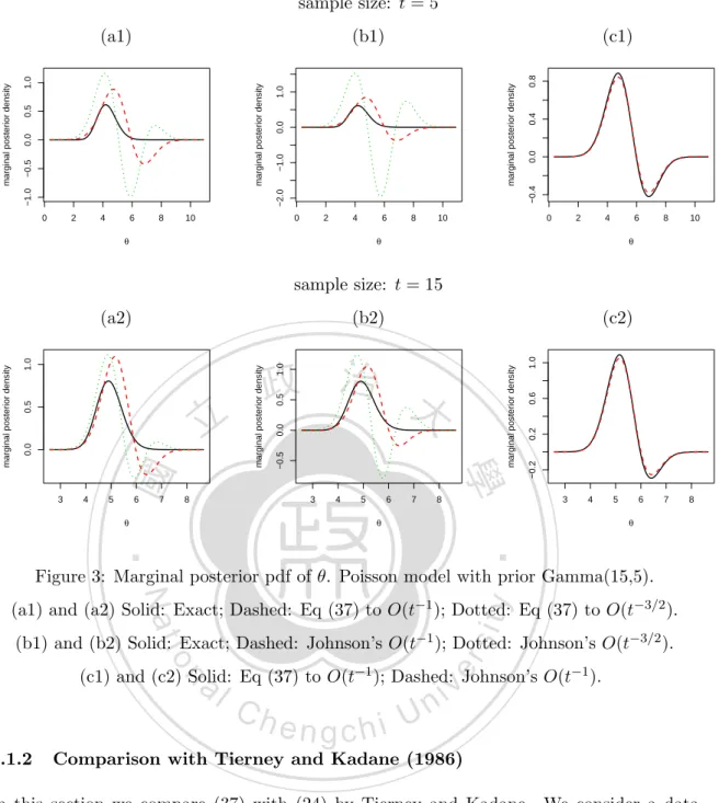
(29) We compare the approximate posterior density of θ by Johnson’s formulas and (37) to orders O(t−1 ) and O(t−3/2 ). Here Johnson’s approximation to O(t−1 ) is obtained by taking K = 1 in (39): pt (w) ≡. dγj (w, x) −1/2 dFt (w) = φ(w) + t + O(t−1 ); dw dw. and the approximation to O(t−3/2 ) is by taking K = 2 in (39). Figures 1(a1) and (a2) give the true density and (37) to O(t−1 ) and O(t−3/2 ); Figures 1(b1) and (b2) give the true density and Johnson’s approximations to O(t−1 ) and O(t−3/2 ); and Figures 1(c1) and (c2) contain the two O(t−1 ) approximations. We have some observations. First, Figures 1(c1) and (c2) show that the two O(t−1 ) approximations are quite close. Secondly, Figure 1(a1) shows that our approximation to O(t−3/2 ) is closer to the true density than approximation to O(t−1 ), but Figure 1(b1) reveals that Johnson’s formula to O(t−3/2 ) does not improve. 治政大and 1). approximations has improved for θ (ranges between 0.5 立 Next we consider a Poisson-Gamma example. Let y , ..., y. upon O(t−1 ). Thirdly, Figures 1(a2) and (b2) show that the negative value of the two. 1. t. be an i.i.d. sample from. ‧ 國. 學. Poisson(θ), where the prior of θ is assumed to be Gamma(a, b). Suppose that (y1 , y2 , y3 , y4 , y5 ) =. ‧. (3, 5, 7, 10, 3) and that (a, b) = (30, 5). Thus, the MLE of θ is 5.6, the prior mean of θ is ∑ 6 and the posterior distribution of θ follows Gamma(a + ti=1 yi , b + t)=Gamma(58,10). We have some observations from Figure 2(a1) to Figure 2(c1). First, Figure 2(c1) indicates. Nat. sit. y. that the two O(t−1 ) approximations are fairly close; secondly, Figure 2(a1) shows that (37). al. er. io. to O(t−3/2 ) improves upon O(t−1 ), but Figure 2(b1) shows that Johnson’s does not.. v. n. Now we try different prior distributions to see its effect on the approximations. Suppose. Ch. i Un. that (a, b) = (15, 5). So, the prior mean of θ is 3 and θ|y ∼ Gamma(43,10). The results are in. engchi. Figures 3(a1) ∼ 3(c1). As before, Figure 3(c1) indicates that the two O(t−1 ) approximations are close. However, due to the fact that the prior mean of θ may be farther from the MLE, from Figures 3(a1) and 3(b1) we found that both O(t−3/2 ) approximations are worse than O(t−1 ). A closer look at these two O(t−3/2 ) curves show that Johnson’s approximation (ranges between -2 and 1.5) fluctuates more widely than ours (ranges between -1 and 1). Next we try different sample sizes for Poisson-Gamma example. We do (y1 , y2 , y3 , y4 , y5 ) = (3, 5, 7, 10, 3) for three times to obtain a sample size 15 with (a, b) = (30, 5) and (15, 5). When (a, b) = (30, 5), the MLE of θ is 5.6, the prior mean of θ is 6 and θ|y follows 22.

(30) Gamma(114,20). Figure 2(c2) indicates that the two O(t−1 ) approximations are close. Figure 2(a2) shows that the negative value of our O(t−3/2 ) approximation has improved for θ ranging between 2 and 4 while Figure 2(b2) shows that the negative value of Johnson’s O(t−3/2 ) approximation has also improved for θ ranging between 7 and 9. When (a, b) = (15, 5), the prior mean of θ is 3 and θ|y follows Gamma(99,20). Figure 3(c2) indicates that the two O(t−1 ) approximations are close. Figure 3(a2) shows that (37) to O(t−3/2 ) shortens the range of negative value according to Figure 3(a1) while Figure 3(b2) shows that Johnson’s also shortens the range of negative value according to Figure 3(b1). In Figure 3, the prior mean of θ is farther from the MLE; the larger the sample size is, the better the result will be. sample size: t = 5 (b1) 治政大. (c1). 5 4. v. 2. 3. engchi. i Un. 0.0. 0.2. 0.4. 0.6. 0.8. 1.0. 2.5 1.5. marginal posterior density. 0.5. 0.2. 0.4. 0.6. 0.8. 1.0. 0.6. 0.8. 1.0. θ. (c2). 0. 0. Ch. 1. marginal posterior density. 5 0. 1. 2. 3. 4. n. er. (b2). al. 0.0. y. sample size: t = 30. io. marginal posterior density. 1.0. θ. Nat. (a2). 0.8. 5. θ. 0.6. 4. 0.4. 3. 0.2. 2. 0.0. −0.5. 2 1 0. 1.0. 1. 0.8. marginal posterior density. 0.6. sit. 0.4. −1. ‧ 國. 0.2. ‧. 0.0. marginal posterior density. 2.5 −0.5. 0.5. 1.5. 立. 學. marginal posterior density. 3. (a1). 0.0. 0.2. θ. 0.4. 0.6 θ. 23. 0.8. 1.0. 0.0. 0.2. 0.4 θ.

(31) Figure 1: Marginal posterior pdf of θ. Beta-Binomial model. (a1) and (a2) Solid: Exact; Dashed: Eq (37) to O(t−1 ); Dotted: Eq (37) to O(t−3/2 ). (b1) and (b2) Solid: Exact; Dashed: Johnson’s O(t−1 ); Dotted: Johnson’s O(t−3/2 ). (c1) and (c2) Solid: Eq (37) to O(t−1 ); Dashed: Johnson’s O(t−1 ). sample size: t = 5. 10. 0. 4. 7. 8. 0.3 0.2 0.0. 2. 4. 6. 8. 10. 7. 8. θ. Ch. (c2) marginal posterior density. 0.8 0.6. y. 0.4. sit. 0.2. marginal posterior density. 0.6 0.4 0.2. marginal posterior density. 0.0. 0.0. 3. 4. n. al. 0. ‧. 6 θ. io. 5. 10. (b2). Nat 4. 8. sample size: t = 15. (a2). 3. 6. θ. 學. ‧ 國. 立. 2. 0.1. marginal posterior density. 0.6 0.4 0.2. 政治大. 5. 6 θ. engchi. 7. 8. i Un. v. 0.6. 8. 0.4. 6 θ. 0.2. 4. 0.0. 2. er. 0. (c1). 0.0. 0.2. 0.4. marginal posterior density. (b1). 0.0. marginal posterior density. (a1). 3. 4. 5. 6 θ. Figure 2: Marginal posterior pdf of θ. Poisson model with prior Gamma(30,5). (a1) and (a2) Solid: Exact; Dashed: Eq (37) to O(t−1 ); Dotted: Eq (37) to O(t−3/2 ). (b1) and (b2) Solid: Exact; Dashed: Johnson’s O(t−1 ); Dotted: Johnson’s O(t−3/2 ). (c1) and (c2) Solid: Eq (37) to O(t−1 ); Dashed: Johnson’s O(t−1 ).. 24.

(32) sample size: t = 5. −2.0 0. 2. 4. 6. 8. 10. 0. 2. 4. 6. θ. 8. 0.8 0.4 0.0 −0.4. 0.0. 1.0. marginal posterior density. (c1). −1.0. −0.5. 0.0. 0.5. marginal posterior density. 1.0. (b1). −1.0. marginal posterior density. (a1). 10. 0. 2. 4. 6. θ. 8. 10. 7. 8. θ. sample size: t = 15. 3. 4. 5. 6. 7. 8. 3. 4. θ. 5. 6. 7. 8. 1.0 0.6 0.2. marginal posterior density. −0.2. 0.0. 0.5. 1.0. 政治大. marginal posterior density. ‧ 國. 0.0. 立. (c2). −0.5. 0.5. 1.0. (b2). 學. marginal posterior density. (a2). 3. 4. θ. 5. 6 θ. ‧. Figure 3: Marginal posterior pdf of θ. Poisson model with prior Gamma(15,5).. Nat. sit. y. (a1) and (a2) Solid: Exact; Dashed: Eq (37) to O(t−1 ); Dotted: Eq (37) to O(t−3/2 ).. al. er. io. (b1) and (b2) Solid: Exact; Dashed: Johnson’s O(t−1 ); Dotted: Johnson’s O(t−3/2 ).. n. (c1) and (c2) Solid: Eq (37) to O(t−1 ); Dashed: Johnson’s O(t−1 ).. 4.1.2. Ch. engchi. i Un. v. Comparison with Tierney and Kadane (1986). In this section we compare (37) with (24) by Tierney and Kadane. We consider a data taken from Mendenhall et al. (1989); see also Tanner (1993). The explanatory variable is the number of days of radiotherapy received by each of 24 patients, and the response variable is the absence (1) and presence (0) of disease at a site three years after treatment. A problem of interest is to use the covariate (days) to predict outcome.. 25.

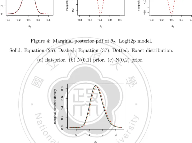
(33) We fit the data using the logistic regression model log. ( p ) i = θ1 + θ2 xi , 1 − pi. where xi is the covariate for patient i and pi is the probability of success (no disease). So, pi = exp(θ1 + θ2 xi )/(1 + exp(θ1 + θ2 xi )). The intercept θ1 represents the log-odds of success for zero days, while the slope θ2 represents the change in the log-odds of success for every unit increase in the covariate. The loglikelihood and the second partial derivatives are `t (θ) =. t t ∑ ∑ [yi logpi + (1 − yi )log(1 − pi )] = [yi (θ1 + θ2 xi ) − log(1 + exp(θ1 + θ2 xi ))], i=1 (2). i=1. `11 = −. ∑. (2). pi (1 − pi ), `12 = −. i. ∑. (2). xi pi (1 − pi ), `22 = −. ∑. i. x2i pi (1 − pi ).. (40). i. Now we take flat priors on both θ1 and θ2 . The comparison of the density in (25) and. 政治大 methods and the true density are very close. Next we take the standard normal density 立 (37) with m = 2 and moments replaced by approximations are in Figure 4(a); the two. priors on both θ1 and θ2 . The results are in Figure 4(b); the result of (25) is close to the. ‧ 國. 學. exact density, but (37) performs poorly. Here the posterior means of qi (Zt2 ), i = 1, ..., 4 are (1.485, 1.460, −0.045, −3.333) and (3.134, 7.207, −0.336, −3.874), respectively. The reason. ‧. why analytic approximation (37) fails may be that the prior mean is farther from the MLE.. y. Nat. If we change priors to N (0, 2), a less informative prior than N (0, 1), then the result of. sit. (37) improves a bit; see Figure 4(c). Since the posterior standard error of θ2 is around. n. al. er. io. 1/23.25 = 0.043, the prior mean 0 is about two standard errors away from θˆt2 . Figure 4. i Un. v. showed that the less informative the prior is (i.e. larger variance), the more accurate the approximate density is.. Ch. engchi. Next we consider a data first analyzed by Finney (1947); see also Albert and Chib (1993) for illustrating a sampling method for marginal posterior densities, and Myers (1990)[p.330332]. A probit model was fit to the data. The model is pi = Φ(θ1 + θ2 c1i + θ3 c2i ), i = 1, ..., 39, where Φ is the cdf of the standard normal density, c1i is the volume of air inspired, c2i is the rate of air inspired, and the binary outcome is the occurrence or non-occurrence on a transient vasorestriction on the skin of the digits. Now we take flat priors on both θ1 and 26.

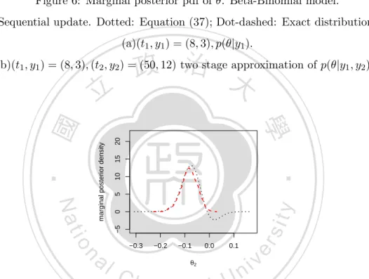
(34) θ2 and obtain the results are in Figure 5, where (37) (with m = 2) is very close to the exact density, but (25) shifts to left slightly.. −0.2. −0.1. 0.0. 0.1. −0.2. −0.1. 0.0. 0.1. 10 20 30 −10 0. marginal posterior density −0.3. θ2. −30. 100 50 0 −50. marginal posterior density. 6 4 2 −0.3. (c). −150. 8. (b). 0. marginal posterior density. (a). −0.3. −0.2. θ2. −0.1. 0.0. 0.1. θ2. Figure 4: Marginal posterior pdf of θ2 . Logit2p model.. 政治大. Solid: Equation (25); Dashed: Equation (37); Dotted: Exact distribution. (a) flat-prior. (b) N(0,1) prior. (c) N(0,2) prior.. 0.8 0.6. 0. 1. n. al. Ch. 2 θ3. 3. er. 0.0. io. sit. 0.2. y. 0.4. ‧. Nat. marginal posterior density. 學. ‧ 國. 立. i Un. v. Figure 5: Marginal posterior pdf of θ3 . Probit model with flat prior. Solid: Equation (25);. engchi. Dashed: Equation (37); Dotted: Exact distribution by numerical integration.. 4.2. Multi-stage Data. The lemma below is well-known. It says that if data D = (D1 , D2 ), then the posterior density of θ given D is the same as the posterior density obtained by taking θ|D1 as the prior and D2 as the data. This result extends to the case D = (D1 , D2 , . . . , Dt ). Suppose that data arrive in different stages. With the first set of data, we can obtain the second 27.

(35) order posterior density approximation by (37). This approximation is considered as the prior density for the next data, and the updating procedure for posterior distribution is repeated by using (37). Lemma 3 Let ξ be the prior for parameter θ and D = (D1 , D2 ) be the observed data. Assuming given θ D1 and D2 are independent. Let L1 (θ) and L2 (θ) be the likelihood functions based on D1 and D2 , respectively. Let ξ(θ|D) be the posterior density of θ given D. Then ξ(θ|D) = 4.2.1. ∫. ξ(θ|D1 )L2 (θ) ξ(θ|D1 )L2 (θ)dθ. (41). Binomial Model. First we consider a binomial model Y ∼ Bin(t, θ), where the prior distribution of θ is. 政治大 p(θ|y) ∝ θ (1 − θ) θ (1 − θ) 立. Beta(α, β). Then, the posterior density for θ is y. β−1. θ|y ∼ Beta(α + y, β + t − y).. ‧. ‧ 國. ∝ θy+α−1 (1 − θ)t−y+β−1 .. 學. So,. t−y α−1. y. Nat. Suppose that t = 58, y = 15, (α, β) = (0.5, 4). So, the posterior distribution of θ given. sit. y is Beta(15.5,47). If the data comes in two stages: Y1 ∼ Bin(8, θ) and Y2 ∼ Bin(50, θ). er. io. with y1 = 3 and y2 = 12, then the posterior distribution of θ given y1 can be approxi-. al. n. iv n C the posterior distribution of θ by h (37) and compareU e n g c h i it with the exact posterior distribution Beta(15.5,47). Figure 6(a) shows the exact and approximate posterior densities of mated by (37). Using this as the prior and y2 as second stage data, we can further update. θ given y1 ; the two densities are close. Here the exact distribution is Beta(3.5,9) with mean 3.5/(3.5+9)=0.28 and mode (3.5-1)/(3.5+9-2)=0.238, and the MLE based on y1 is 3/8=0.375. Figure 6(b) shows the densities of exact posterior distribution Beta(15.5,47) and our two-stage approximation. Here the MLE based on y is 15/58=0.259 and the mean of Beta(15.5,47) is 15.5/(15.5+47)=0.248. We also conducted more experiments and found that the approximation (37) may not perform well when the posterior mode in the previous data greatly differs from the MLE of second-stage data. 28.

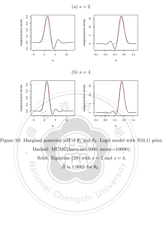
(36) 4.2.2. Two-parameter Logit Model. To update posterior density for two-parameter problems in the two-stage scenario, we need to have an approximate joint posterior density at the first stage, which will be considered as the prior in the second stage. Such an approximation can be obtained by (35) with posterior moments replaced by their approximations; that is, 2 ˆ t Zt + q1 (z2∗ )E ˆ t Zt + 1 q2 (z1∗ )(E ˆ t Zt1 ξˆt (θ1 , θ2 ) = |Σt |φ2 (z ∗ )[1 + q1 (z1∗ )E − 1) ξ 1 ξ 2 ξ 2 ˆ t Zt1 Zt2 ) + 1 q2 (z ∗ )(E ˆ t Z 2 − 1) +q1 (z1∗ )q1 (z2∗ )(E 2 ξ ξ t2 2 1 1 ˆ t Z 3 − 3E ˆ t Zt1 ) + q2 (z ∗ )q1 (z ∗ )(E ˆ t Z 2 Zt2 − E ˆ t Zt2 ) (42) + q3 (z1∗ )(E 1 2 ξ t1 ξ ξ t1 ξ 6 2 1 ˆ t Zt1 Z 2 − E ˆ t Zt1 ) + 1 q3 (z ∗ )(E ˆ t Z 3 − 3E ˆ t Zt2 )]. + q1 (z1∗ )q2 (z2∗ )(E t2 2 ξ ξ ξ t2 ξ 2 6. 治政 tives; see Weng (2010b) and Weng and Hsu (2011). 大立 the same data from Mendenhall et al. (1989) as in Section In the first stage, we consider The moment approximations are in terms of the loglikelihood and the prior and their deriva-. ‧ 國. 學. 4.1.2. The data D1 contains 24 observations. We take flat priors on both θ1 and θ2 and obtain an approximate joint posterior density ξˆt (θ1 , θ2 ) by (42). Next we use this approxi-. ‧. mation as prior and randomly select 18 observations from D1 as the data of second stage, denoted as D2 . Then we update the posterior density of θ by (42). Since the exact pos-. y. Nat. sit. terior density does not have a closed form, we compare our two-stage approximation with. al. er. io. MCMC results using MCMCpack (2010). The results are in Figure 7. We found that the. n. two densities are rather close, but the approximation method may sometimes give negative values.. 4.3. Ch. engchi. i Un. v. Logit Model. Two-parameter case. Consider the same logit model in Section 4.1.2. We take flat priors on both θ1 and θ2 and use the implied density (29) to validate convergence of MCMC samples. To begin, we run the MCMClogit function in an R package MCMCpack (2010) to this data and obtain the posterior of MCMC samples. The comparisons of the density of MCMC samples and the implied density (29) are in Figures 8 and 9, based on posterior samples of sizes 100 (burn-in=50) and 10000 (burn-in=5000), respectively. Here [Σt ]22 = 23.25, 29.

(37) θˆt2 = −0.085, and the posterior means of qi (Zt2 ), i = 1, . . . , 10 from the MCMC samples in ˆ Figure 9 are (-0.224, 0.198, -0.416, 0.329, -0.069, -0.646, 2.844, -3.699, -6.565, 36.080) and R is 1.0020 for θ2 . The sample sizes and burn-in are chosen so that one exhibits convergence, but one does not. As expected, Figure 9 with s = 2 and s = 4 shows nice agreement; however, for Figure 8, the posterior sample and the implied density (29) with s = 2, s = 4, ˆ is 1.2309 for θ2 . Now we take the standard s = 20 and s = 27 are disagreements and R normal priors on both θ1 and θ2 and use the implied density (29) to validate convergence of MCMC samples. The comparisons of the density of the posterior samples (size=10000, burn-in=5000) and the implied density (29) with s = 2 and s = 4 are in Figure 10. Here the posterior means of qi (Zt2 ), i = 1, . . . , 10 from the MCMC samples are (1.507, 1.535, ˆ is 1.0001 for θ2 . The 0.095, -3.243 , -5.175, 4.035, 28.610, 22.206, -132.075, -336.186) and R. 政治大. posterior samples has converged, but the implied density (29) failed to diagnose for this example.. 立. Three-parameter case. Next, we consider the data analyzed by Finney (1947). A logistic. ‧ 國. 學. regression was fit to the data. The model is. ‧. ( p ) i log = θ1 + θ2 c1i + θ3 c2i , i = 1, . . . , 39. 1 − pi. The residual deviance gives a χ2 -value of 29.772 with 36 degrees of freedom, indicating that. Nat. sit. y. the logistic model is quite adequate. The comparisons of the density of MCMC samples. io. er. (size=10000, burn-in=5000) and the implied density (29) with s = 2 and s = 4 are in Figure 11. The implied density (29) failed to diagnose for this example. The reason might. n. al. i Un. v. be that the posterior density has quite heavy tails. Here [Σt ]33 = 1.093, θˆt3 = 2.649, and the. Ch. engchi. posterior means of qi (Zt3 ), i = 1, . . . , 10 from the MCMC samples in Figure 11 are (0.557, ˆ is 1.0023 0.666, 1.886, 5.581, 18.701, 73.833, 318.033, 1444.880, 6826.201, 32712.78) and R for θ3 . As a remedy, we truncate some extreme values from the MCMC samples. The comparisons of the density of MCMC samples (size=10000, burn-in=5000) and the implied density (29) with s = 2 and s = 4 are in Figure 12. Using a larger s gives better results. Here the posterior means of qi (Zt3 ), i = 1, . . . , 10 from the MCMC samples in Figure 12 are (0.399, 0.086, 0.025, -0.381, -1.335, -0.560, 6.126, 13.857, -11.231, -116.282).. 30.

(38) We truncate some extreme values from the MCMC samples to get better results on logit3p model at present section. We have a further discussion on this example and propose a method that transforms Zt to another pivotal quantity in chapter 5. Now we take the standard normal priors on θ1 , θ2 , and θ3 , and use the implied density (29) to validate convergence of MCMC samples. Here the posterior means of qi (Zt3 ), i = 1, . . . , 10 from MCMC samples are (-2.257, 4.217,-5.564, 1.478, 16.393, -43.238, 11.314, ˆ is 1.0013 for θ3 . In this example the posterior samples 241.204, -627.421, -488.959) and R have heavy tails so we truncate some samples from the MCMC samples. Here the posterior means of qi (Zt3 ), i = 1, . . . , 10 from the MCMC samples are (-2.279, 4.299, -5.719, 1.509, 16.952, -45.244, 12.290, 253.552, -662.408, -522.589). The comparisons of the density of MCMC samples and the implied density (29) with s = 2, s = 4 and s = 14 are in Figure. 政治大. 13, based on posterior samples of sizes 10000 (burn-in=5000). Six-parameter case. Next, we consider a six-parameter problem. Kutner et al. (2004). 立. studied the strength of association between several risk factors and the duration of preg-. ‧ 國. 學. nancies based on 102 women. The risk factors were nutritional status (x1 ), mother’s age (categorized into three groups and represented by two indicator variables x2 and x3 ), history. ‧. of alcohol use (x4 ), and history of tobacco use (x5 ). The response of interest, pregnancy duration, was originally categorized into three groups: preterm (less than 36 weeks), inter-. Nat. sit. y. mediate term (from 36 to 37 weeks), and full term (38 weeks or greater). Here we combine. io. er. the first two categories (coded 1) and let the full term be the second group (coded 0), and then fit a logistic regression model to the data. For details, see Kutner et al. (2004). The. al. n. model is. Ch. engchi. i Un. v. ( p ) i = θ1 + θ2 x1i + θ3 x2i + θ4 x3i + θ5 x4i + θ6 x5i , i = 1, . . . , 102. log 1 − pi We run MCMCpack (2010) to obtain posterior samples of sizes 10000 (burn-in=10000). Figure 14 shows that the implied density (29) with s = 4 is quite close to the MCMC result. For example, for θ6 we have [Σt ]66 = 1.586, θˆt6 = 2.309, and the posterior means of qi (Zt6 ) for i = 1, ..., 4 from the MCMC samples in Figure 14 are (0.407, 0.237, 0.367, 0.610) ˆ is 1.0114. With these six numbers, we can capture the posterior density of θ6 pretty and R well.. 31.

(39) 4.4. Poisson Regression Model. We consider a data taken from Hinde (1982). The explanatory variable is the length of each roll, and the response variable is the numbers of faults found in 32 rolls of fabric produced in a particular factory. A problem of interest is the number of faults to be proportional to the length of roll. We fit the data using the poisson regression model log(µi ) = θ1 + θ2 xi where xi is the length of ith roll and µi is the mean of related response variable. The intercept θ1 represents the log-mean for zero length roll, while the slope θ2 represents the change in the log-mean of response variable for every unit increase in the covariate. The loglikelihood and the second partial derivatives are `t (θ) = θ1. t ∑. 立. t. i=1 (2). i=1. exp(θ1 + θ2 xi ), `12 = −. ‧ 國. i=1. t. i i. t ∑. 1. 2 i. i=1. (2). xi exp(θ1 + θ2 xi ), `22 = −. 學. (2). `11 = −. t ∑. ∑ 政∑ x 治 y − exp(θ + θ x ) + C, 大. yi + θ2. i=1. t ∑. x2i exp(θ1 + θ2 xi ).. i=1. Now we take flat priors on both θ1 and θ2 and use the implied density (29) to validate. ‧. convergence of MCMC samples. We run WinBUGS Lunn et al. (2000) to obtain the posterior. y. Nat. MCMC samples of sizes 10000 (burn-in=5000). Figures 15(a2) and (b2) show that the. sit. implied density (29) with s = 2 and s = 4 is quite close to the density of posterior samples.. al. er. io. Here we have [Σt ]22 = 3264.80 and θˆt2 = 0.0019, and the posterior means of qi (Zt2 ),. v. n. i = 1, ..., 4 from the MCMC samples in Figure 15(b2) are (0.052, −0.014, 0.047, 0.044) and. Ch. i Un. ˆ is 1.0004 for θ2 . Now we take the standard normal priors on both θ1 and θ2 and use the R. engchi. implied density (29) to validate convergence of MCMC samples. Figures 16(a2) and (b2) show that the implied density (29) with s = 2 and s = 4 is very close to the MCMC result. Here the posterior means of qi (Zt2 ), i = 1, . . . , 4 from the MCMC samples in Figure 16(b2) ˆ is 1.0011 for θ2 . are (0.235, 0.021, −0.026, −0.080) and R Given sample size t = 16, we randomly draw 16 observations from Hinde (1982). As before, we take flat priors on both θ1 and θ2 . Figures 15(a1) and (b1) show that the implied density (29) with s = 2 and s = 4 is quite close to the density of posterior samples. Here we have [Σt ]22 = 2487.49 and θˆt2 = 0.00199, and the posterior means of qi (Zt2 ), i = 1, ..., 4 32.