三層類神經網路的動態最佳學習

全文

(1)國立交通大學電機與控制工程學系碩士論文. 三層類神經網路的動態最佳學習. Dynamic Optimal Training of A Three Layer Neural Network with Sigmoid Function. 研究生：紀右益指導教授：王啟旭. 教授. 中華民國九十四年六月.

(2) 三層類神經網路的動態最佳學習. Dynamic Optimal Training of A Three Layer Neural Network with Sigmoid Function. 研究生：紀右益. Student: Yu-Yi Chi. 指導教授：王啟旭. 教授. Advisor: Chi-Hsu Wang. 國立交通大學電機與控制工程學系碩士論文. A Thesis Submitted to Department of Electrical and Control Engineering College of Electrical Engineering and Computer Science National Chiao Tung University in Partial Fulfillment of the Requirements for the Degree of Master in Electrical and Control Engineering June 2005 Hsinchu, Taiwan, Republic of China. 中華民國九十四年六月.

(3) 三層類神經網路的動態最佳學習. 研究生：紀右益. 指導教授：王啟旭教授. 國立交通大學電機與控制工程研究所. 摘要本篇論文是針對三層類神經網路提出一個動態最佳訓練法則，其中網路的隱藏層和輸出層都有經過一個 S 型激發函數。這種三層的網路可以被運用於處理分類的問題，像是蝴蝶花的品種分類。我們將對這種三層神經網路的動態最佳訓練方法提出一個完整的証明，用來說明這種動態最佳訓練方法保證神經網路能在最短的迭代次數下達到收斂的輸出結果。這種最佳的動態訓練方法不是使用單一固定的學習速率，而是在每一次的迭代過程中不斷的更新，來取得下一次迭代過程所需要的最佳學習速率，以保證最佳的收斂的訓練結果。我們可以由 XOR 和蝴蝶花的測試例子得到良好的結論。. i.

(4) Dynamic Optimal Training of A Three Layer Neural Network with Sigmoid Function. Student: Yu-Yi Chi. Advisor: Chi-Hsu Wang. Department of Electrical and Control Engineering National Chiao Tung University. ABSTRACT This thesis proposes a dynamical optimal training algorithm for a three layer neural network with sigmoid activation functions in the hidden and output layers. This three layer neural network can be used for classification problems, such as the classification of Iris data. Rigorous proof has been presented for the dynamical optimal training process for this three layer neural network, which guarantees the convergence of the training in a minimum number of epochs. This dynamical optimal training does not use fixed learning rate for training. Instead, the learning rates are updated for next iteration to guarantee the optimal convergence of the training result. Excellent results have been obtained for XOR and Iris data set.. ii.

(5) ACKNOWLEDGEMENT. I feel external gratitude to my advisor, Chi-Hsu Wang for teaching me many things. He taught me how to do to the research and the most important is that he taught me how to get along with people. And I am grateful to everyone in ECL. I am very happy to get along with you. Finally, I appreciate my parent’s support and concern, therefore I can finish my master degree smoothly.. iii.

(6) TABLE OF CONTENTS ABSTRACT (IN CHINESE) ..........................................................................................i ABSTRACT...................................................................................................................ii ACKNOWLEDGEMENT ........................................................................................... iii TABLE OF CONTENTS ..............................................................................................iv LIST OF TABLES .........................................................................................................v LIST OF FIGURES ......................................................................................................vi CHAPTER 1 Introduction..............................................................................................1 CHAPTER 2 The Perceptron as A Neural Network ......................................................3 2.1. Single Layer Perceptron..................................................................................3 2.2. The Simple Examples .....................................................................................6 2.3. Multi-layer Feed-Forward Perceptrons...........................................................8 2.4. The Back-Propagation Algorithm (BPA) ........................................................9 CHAPTER 3 Dynamic Optimal Training of A Three-Layer Neural Network with Sigmoid Function.........................................................................................................14 3.1. The Architecture of A Three-Layer Network................................................14 3.2. The Dynamic Optimal Learning Rate...........................................................15 3.3. Dynamical Optimal Training via Lyapunov’s Method .................................19 CHAPTER 4 Experimental Results .............................................................................22 4.1. Example 1: The XOR Problem .....................................................................22 4.2. Example 2: Classification of Iris Data Set....................................................31 CHAPTER 5 Conclusions............................................................................................42 REFERENCES ............................................................................................................43. iv.

(7) LIST OF TABLES TABLE 2.1 THE TRUTH TABLE FOR AND .........................................................................................6 TABLE 2.2 THE TRUTH TABLE FOR XOR.........................................................................................7 TABLE 4.1. THE TRAINING RESULT FOR XOR USING DYNAMICAL OPTIMAL TRAINING.27 TABLE 4.2. THE TRAINING RESULT FOR XOR USING FIXED LEARNING RATE Β = 0.9 .......28 TABLE 4.3. ACTUAL AND DESIRED OUTPUTS AFTER 10000 ITERATIONS..............................37 TABLE 4.4. ACTUAL AND DESIRED OUTPUTS IN REAL TESTINGS..........................................39. v.

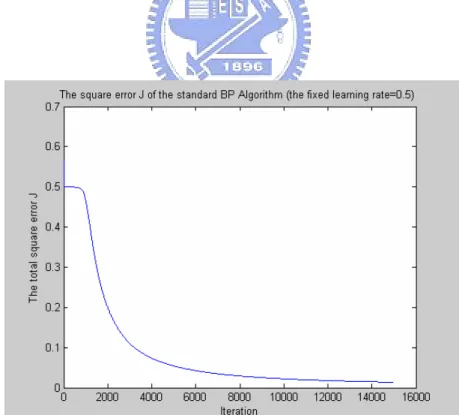
(8) LIST OF FIGURES FIGURE 2-1-1. SINGLE LAYER PERCEPTRON..................................................................................3 FIGURE 2-1-2. ANOTHER MODEL OF SINGLE LAYER PERCEPTRON.........................................4 FIGURE 2-2. THE HARD LIMITER FOR PERCEPTRON ...................................................................4 FIGURE 2-3. THE DECISION BOUNDARY FOR 2-DEMENSIONAL PLANE..................................5 FIGURE 2-4. THE INPUT DATA OF AND ............................................................................................6 FIGURE 2-5. THE ARCHITECTURE OF THE NETWORK FOR SOLVING AND LOGIC PROBLEM......................................................................................................................................7 FIGURE 2-6. THE INPUT DATA OF XOR ............................................................................................7 FIGURE 2-7. A THREE LAYER FEED-FORWARD NETWORK .........................................................8 FIGURE 2-8. THE SIGMOID FUNCTION.............................................................................................9 FIGURE 3-1. THE THREE LAYER NEURAL NETWORK ................................................................14 FIGURE 4-1. THE DISTRIBUTION OF XOR INPUT DATA SETS ...................................................22 FIGURE 4-2. THE NEURAL NETWORK FOR SOLVING XOR .......................................................23 FIGURE 4-3-1. THE SQUARE ERROR J OF THE STANDARD BPA WITH FIXED β = 1.5 ...........23 FIGURE 4-3-2. THE SQUARE ERROR J OF THE STANDARD BPA WITH FIXED β = 0.9 ...........24 FIGURE 4-3-3. THE SQUARE ERROR J OF THE STANDARD BPA WITH FIXED β = 0.5 ...........24 FIGURE 4-3-4. THE SQUARE ERROR J OF THE STANDARD BPA WITH FIXED β = 0.1 ...........25 FIGURE 4-4. THE SQUARE ERROR J OF THE BPA WITH DYNAMIC OPTIMAL TRAINING ...25 FIGURE 4-5. THE DIFFERENCE EQUATION G(Β(N)) AND βOPT = 7.2572.....................................26 FIGURE 4-6. THE DYNAMIC LEARNING RATES OF EVERY ITERATION..................................26 FIGURE 4-7. TRAINING ERRORS OF DYNAMIC OPTIMAL LEARNING RATES AND FIXED LEARNING RATES.....................................................................................................................27 FIGURE 4-8-1. THE SQUARE ERROR J OF THE BPA WITH VARIANT MOMENTUM(β = 0.9) ...29 FIGURE 4-8-2. THE SQUARE ERROR J OF THE BPA WITH VARIANT MOMENTUM(β = 0.5) ...29 FIGURE 4-8-3. THE SQUARE ERROR J OF THE BPA WITH VARIANT MOMENTUM (β = 0.1) ..30 FIGURE 4-9. TOTAL SQUARE ERRORS OF DYNAMIC TRAINING AND THE BPA WITH DIFFERENT LEARNING RATES AND MOMENTUM ............................................................30 FIGURE 4-10-1. THE TOTAL IRIS DATA SET (SEPAL) ....................................................................31 FIGURE 4-10-2. THE TOTAL IRIS DATA SET (PETAL)....................................................................32 FIGURE 4-11-1. THE TRAINING SET OF IRIS DATA (SEPAL) .......................................................32 FIGURE 4-11-2. THE TRAINING SET OF IRIS DATA (PETAL) .......................................................33 FIGURE 4-12. THE NEURAL NETWORK FOR SOLVING IRIS PROBLEM...................................33 FIGURE 4-13-1. THE SQUARE ERROR J OF THE STANDARD BPA WITH FIXED β = 0.1 .........34 FIGURE 4-13-2. THE SQUARE ERROR J OF THE STANDARD BPA WITH FIXED β = 0.01 .......34 FIGURE 4-13-3. THE SQUARE ERROR J OF THE STANDARD BPA WITH FIXED β = 0.001 .....35 FIGURE 4-14. THE SQUARE ERROR J OF THE BPA WITH DYNAMIC OPTIMAL TRAINING .35. vi.

(9) FIGURE 4-15. TRAINING ERRORS OF DYNAMIC OPTIMAL LEARNING RATES AND FIXED LEARNING RATES.....................................................................................................................36. vii.

(10) CHAPTER 1 Introduction Artificial neural network (ANN) is the science of investigating and analyzing the algorithms of the human brain, and using the similar algorithm to build up a powerful computational system to do the tasks like pattern recognition [1], [2], identification [3], [4] and control of dynamical systems [5], [6], system modeling [7], [8] and nonlinear prediction of time series [9]. The artificial neural network owns the capability, to organize its structural constituents, the same as the human brain. So the most attractive character of artificial neural network is that it can be taught to achieve the complex tasks we just experienced before by using some learning algorithms and training examples. The learning algorithms here can be roughly divided into two parts: one is the supervised learning and the other is the unsupervised learning. One most popular algorithm of artificial neural network for classification is the Error Back-Propagation Algorithm [10], [11], which is the supervised learning. The well-known error back-propagation algorithm, or simply the back-propagation algorithm, for training multi-layer perceptrons was proposed by Rumelhart in 1986 [12]. The back-propagation algorithm is a generalized form of the delta learning rule, which is actually based on the least-mean square algorithm. The topic of the training process is to minimize the standard mean-square error. Although the way to adjust the weights of network, i.e., the method of steepest descent, is easy to understand, there are several flaws in the back-propagation algorithm. One of them is that we don’t have a suitable way to find the stable and optimal learning rate. For smaller learning rate, we may have a convergent result. But the speed of the output convergence is very slow and need more number of epochs to train the network. For larger learning rate, the speed of training can be accelerated, but it will cause the training result to fluctuate and even leads to divergent result. Actually the dynamical optimal training was proposed in [13] for a simple two layer neural network (without hidden layers) without any activation functions in the output layer. The basic theme in [13] is to find a stable and optimal learning for the next iteration in back propagation algorithm. Moreover a more complicated three layer neural network (with one hidden layer) with sigmoid activation functions in the hidden and output layers is very useful in performing the classification problems, such as the XOR [14] and Iris data [15], [16]. However its learning process has been very slow in terms of the classical back propagation algorithm. In other words, the dynamical optimal learning algorithm has never been proposed for this type of neural network. Therefore the major purpose of this thesis is to find a proper way to achieve the dynamical optimal training of the 1.

(11) three layer neural network with sigmoid activation functions in hidden and output layers. Rigorous proof will be proposed and the popular XOR and Iris data classification benchmarks will be fully illustrated. Excellent results have been obtained by comparing our optimal training results with previous results using fixed small learning rates.. 2.

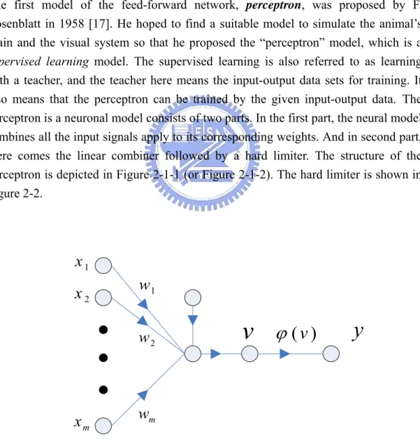
(12) CHAPTER 2 The Perceptron as A Neural Network In this chapter, the multi-layer feed-forward perceptrons will be introduced. First the single layer perceptron will be explained and it will lead to the multi-layer perceptrons in later sections. Also the back propagation algorithm for multi-layer feed forward perceptrons will be explained in section 2.4. 2.1. Single Layer Perceptron The first model of the feed-forward network, perceptron, was proposed by F. Rosenblatt in 1958 [17]. He hoped to find a suitable model to simulate the animal’s brain and the visual system so that he proposed the “perceptron” model, which is a supervised learning model. The supervised learning is also referred to as learning with a teacher, and the teacher here means the input-output data sets for training. It also means that the perceptron can be trained by the given input-output data. The perceptron is a neuronal model consists of two parts. In the first part, the neural model combines all the input signals apply to its corresponding weights. And in second part, there comes the linear combiner followed by a hard limiter. The structure of the perceptron is depicted in Figure 2-1-1 (or Figure 2-1-2). The hard limiter is shown in Figure 2-2.. x1 x2. w1. v. w2. xm. ϕ (v ). wm Figure 2-1-1. Single layer perceptron. 3. y.

(13) x0 = 1 x1. x2. w0 = b w1. v. w2. ϕ (v ). y. wm xm Figure 2-1-2. Another model of single layer perceptron. Figure 2-2. The hard limiter for perceptron In Figure 2-1-1, the input data set of the perceptron is denoted by {x1, x2,…, xm} and the corresponding synaptic weights of the perceptron are denoted by{w1, w2,…, wm}. The external bias is denoted by b. The first part of the percpetron computes the linear combination of the products of input data and synaptic weight with an externally applied bias. So the result of the first part of the perceptron, v, can be expressed as m. v = b + ∑ wi xi. (2.1). i =1. Then in the second part, the resulted sum v is applied to a hard limiter. Therefore, the output of the perceptron equals +1 or 0. The output of perceptron equals to +1 if the resulted sum v is positive or zero; and the output of perceptron equals to 0 if v is negative. This can be simply expressed by (2.2). 4.

(14) m ⎧ + 1 ， if b + xi wi ≥ 0 ∑ ⎪ ⎪ i=1 (2.2) y=⎨ m ⎪ 0 ，if b + x w < 0 ∑ i i ⎪⎩ i=1 The goal of the perceptron is to classify the input data point represents by the set {x1,. x2,…, xm} into one of two classes, C1 and C2. If the output of the perceptron equals to +1, the input data point represented by the set {x1, x2,…, xm}will be assigned to class C1. Otherwise, the input data point will be assigned to class C2. Since the classification depends on the output of the perceptron, y, and the output y is decided by the resulted sum v. If we only consider the simplest form of the perceptron, the m-dimensional space can only be divided into two decision regions by the hyper-plane, which is defined as m. b +∑ xi wi = 0. (2.3). i=1. One simple example is shown in Figure 2-3. In this case, there are only two input variables x1 and x2 for single layer perceptron, for which the decision hyper-plane is a straight line. The hyper-plane can be shown as: b + x1w1 + x2 w2 = 0 (2.4) Note that the shift distance of the decision line away from the origin is decided by the parameter b in (2.4) (and (2.3)).. Class 1 Class 2 Hyperplane. X2. X1 Figure 2-3. The decision boundary for 2-demensional plane For convenience, we can consider the architecture of single layer perceptron in another form as depicted in Figure 2-1-2 and (2.1) can be rewritten as m. v = ∑ wi xi i =0. 5. (2.5).

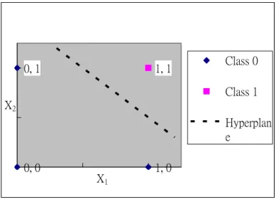
(15) In which, we substitute w0 for the term b in (2.3) and x0 = 1. The other results are all the same [18]. 2.2. The Simple Examples Example 1. The AND Problem The AND logic problem, which can be solved by the single layer perceptron easily. The truth table for AND is shown in Table 2.1. Table 2.1 The truth table for AND A. B. 0. 0. 0 (Class 0). 0. 1. 0 (Class 0). 1. 0. 0 (Class 0). 1. 1. 1 (Class 1). A AND. B. The input data set of the AND logic is shown in Figure 2-4, which is obviously a linearly separable problem. For solving this problem, we can build the single layer perceptron by assigning the suitable synaptic weights with external bias for. The architecture of the network is illustrated in Figure 2-5, in which the synaptic weights are assigned as w1 = w2 = 1 and the external bias b= -1.5. Besides the AND logic, the OR and NOT logic problems are also linear separable. So these three logic problems can be solved by the same way easily. The only difference is the choice of the synaptic weights w1, w2 and external bias b.. 0, 1. 1, 1. Class 0 Class 1. X2. Hyperplan e 0, 0. 1, 0. X1. Figure 2-4. The input data of AND. 6.

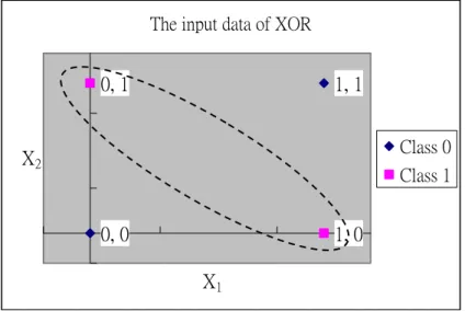
(16) Figure 2-5. The architecture of the network for solving AND logic problem Example 2. The XOR Problem The Exclusive OR (XOR) logic problem can’t be solved by single layer perceptron because the XOR logic is with nonlinear separable input data set. The truth table for XOR is shown in Table 2.2. Table 2.2 The truth table for XOR A. B. 0. 0. 0 (Class 0). 0. 1. 1 (Class 1). 1. 0. 1 (Class 1). 1. 1. 0 (Class 0). A XOR. B. From Figure 2-6, we can see that the input data is not linear separable. So, the single layer perceptron can not work for this problem. We can not find the suitable parameters w1, w2 and b to classify the output y in Figure 2-6.. The input data of XOR. 0, 1. 1, 1 Class 0. X2. Class 1. 0, 0. 1, 0 X1. Figure 2-6. The input data of XOR. 7.

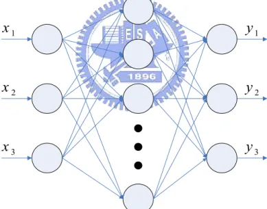
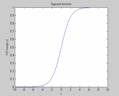
(17) From the statements of section 2.1 and 2.2, we know that the single layer perceptron can only solve the problems which are linear separable. Besides this, another serious defect is that we have no proper learning algorithm to adjust the synaptic weights for the single layer perceptron, and all the parameters can only be assigned by try-and-error method. Until 1985, this problem was solved when the Back-Propagation algorithm was proposed. So the single layer perceptron was gradually replaced by Back-Propagation algorithm in the present day. 2.3. Multi-layer Feed-Forward Perceptrons In this section we will introduce the multi-layer feed-forward network, an important class of neural network. The difference between single layer perceptron and multi-layer feed-forward perceptrons is the “hidden layer”. The multi-layer network consists of a set of input nodes (input layer), one or more hidden layers, and a set of output nodes that constitute the output layer. The input signals will propagate through the network in the forward direction. A multi-layer feed-forward fully-connected network is shown in Figure 2-7 with only one hidden layer.. x1. y1. x2. y2. x3. y3. Figure 2-7. A three layer feed-forward network The major characters of the multi-layer network are as follow: (1) Besides the neurons of input layer, every neuron of the network has a nonlinear activation function. Note that the activation function used in the multi-layer network is smooth, means the activation function is differentiable everywhere, which is different from the activation function for single layer perceptron, the hard limiter shown in Fig. 2-2. The most popularly activation function is the 8.

(18) sigmoid function, whose graph is s-shaped, as shown in Figure 2-8 with 1 y= 1 + exp(− ax). (2.6). where y is the output signal of the neuron and v is the input signal. And the parameter a is the slop parameter of the sigmoid function. We can get different sigmoid functions by varying the slop parameter a, but we usually choose the sigmoid function with a = 1. Equation (2.6) is defined as a strictly increasing function that exhibits a graceful balance between linear and nonlinear behaviors. (2) The multi-layer network contains at least one hidden layer which is between input layer and output layer. The hidden layers enable the multi-layer networks to deal with more complex problems which can not be solved by single layer perceptron. The number of hidden layers for different problems is also an open question. We choose only one hidden layer with sigmoid activation functions in the hidden and output layers to solve the classification problem in this paper. This three layer perceptrons is also the most popular neural network adopted for many engineering applications.. Figure 2-8. The sigmoid function 2.4. The Back-Propagation Algorithm (BPA) The most serious problem of the single layer perceptron is that we don’t have any proper learning algorithm to adjust the synaptic weights of the perceptron. But the multi-layer feed-forward perceptrons don’t have this problem. The synaptic weights of the multi-layer perceptrons can be trained by using the highly popular algorithm known as the error back-propagation algorithm (EBP algorithm). We can view the error back-propagation algorithm as the general form of the least-mean square 9.

(19) algorithm (LMS). The error back-propagation algorithm (or the back-propagation algorithm) consists of two parts, one is the forward pass and the other is the backward pass. In the forward pass, the effect of the input data propagates through the network layer by layer. During this process, the synaptic weights of the networks are all fixed. On the other hand, the synaptic weights of the multi-layer perceptrons are all adjusted in accordance with the error-correction rule during the backward pass. Before using error-correction rule, we have to define the error signal of the learning process. Because the goal of the learning algorithm is to find one set of weights which makes the actual outputs of the network equal to the desired outputs, so we can define the error signal as the difference between the actual output and the desired output. Specifically, the desired response is subtracted from the actual response of the network to produce the error signal. In the backward pass, the error signal propagates backward through the network from output layer. During the backward pass, the synaptic weights of the multi-layer perceptrons are adjusted to make the actual outputs of the network move closer to the desired outputs. This is why we call this algorithm as “error back-propagation algorithm”. Now, we will consider the learning process of the back-propagation algorithm. First, the error signal at the output node j at the tth iteration is defined by. e j ( t ) = y mj ( t ) − d j ( t ). (2.7). where dj is the desired output of output node j and ymj is the actual output of output node j. The ymj can also be represented as: 1 y mj = ϕ (net mj ) = (2.8) 1 + exp(−net mj ) Where the term ψ(．) is the activation function, which is the sigmoid function, and netmj is the output of node j in output layer. We can rewrite (2.8) as a more general form: 1 y kj = ϕ ( net kj ) = (2.9) 1 + exp(−net kj ) where ykj is the output of node j in the kth layer and netkj is the linear combination output of node j in the kth layer, which can be expressed as net kj = ∑ wkji yik −1 − b kj. (2.10). i. In (2.10), the term wkji is the synaptic weight between the jth neuron in the kth layer and the ith neuron in the (k-1)th layer, and bkj is the external bias of the jth neuron in the kth layer. Then we can define the square error of neuron j in output layer by: 1 2. ζ j = e 2j ( t ). 10. (2.11).

(20) By the same way, we can define the total square error J of the network as: 1 J = ∑ ζ j = ∑ e 2j 2 j j. (2.12). The goal of the back-propagation algorithm is to find one set of weights so that the actual outputs can be as close as possible to the desired outputs. In other words, the purpose of the back-propagation algorithm is to reduce the total square error J, as described in (2.12). In the method of steepest descent, the successive adjustments applied to the weight matrix W are in the direction opposite to the gradient matrix ∂J / ∂W . The adjustment can be expressed as: ∂J ∆W ( t ) = −η (2.13) ∂W t where η is the learning rate parameter of the back-propagation algorithm. It decides the step-size of correction of the method of steepest descent [18]. Note that the learning rate is a positive constant. By using the chain rule, the element of matrix ∂J ∂W , i.e. ∂J ∂wkji , can be represented as k k ∂J ∂J ∂y j ∂net j = ∂wkji ∂y kj ∂net kj ∂wkji. (2.14). We can rewrite ∂y kj ∂net kj by using (2.9) to have ∂y kj ∂net. k j. = ϕ ' ( net kj ) =. ∂ ∂net kj. ⎛ ⎞ 1 = y kj (1 − y kj ) ⎜⎜ k ⎟ ⎟ ⎝ 1 + exp( − net j ) ⎠. (2.15). We can also rewrite ∂net kj ∂w kji by using (2.10) to have. ∂net kj ∂w. k ji. =. ∂ ⎛ ⎞ wkji yik −1 − b j ⎟ = yik −1 k ⎜∑ ∂w ji ⎝ i ⎠. (2.16). The item ∂J / ∂y kj in (2.14) can be discussed separately for two cases: 1.. If kth layer is the output layer, then k = m and ykj = ymj. So we can substitute (2.12) into ∂J / ∂y kj to have. ∂J ∂ = k k ∂y j ∂y j 2.. ⎡1 2⎤ m m ⎢ ∑( yj − d j ) ⎥ = ( yj − d j ) 2 ⎣ j ⎦. (2.17). If the kth layer is not output layer which means the kth layer is one of the hidden 11.

(21) layers. So, by using the chain rule we can rewrite ∂J / ∂y kj as ⎛ ∂J ∂netlk +1 ⎞ ∂J = ∑l ⎜⎜ ∂net k +1 ∂y k ⎟⎟ ∂y kj l j ⎝ ⎠. (2.18). By using (2.10), the term ∂netlk +1 ∂y kj ∂netlk +1 ∂ ⎛ ⎞ = k ⎜ ∑ wlik +1 yik − blk +1 ⎟ = wljk +1 k ∂y j ∂y j ⎝ i ⎠. (2.19). where wk+1lj is the synaptic weight between the jth neuron in the (k+1)th layer and the lth neuron in the kth layer. For simplicity, we assume the item ∂J / ∂netlk +1 in (2.18) to have the following form: ∂J = δ lk +1 k +1 ∂netl. Substitute (2.19) and (2.20) into (2.18), we have ∂J = ∑ (δ lk +1wljk +1 ) k ∂y j l. (2.20). (2.21). From (2.14) to (2.21), we have the following observations: 1. If the synaptic weights are between the hidden layer and output layer, then ∂J = ( y mj − d j ) y kj (1 − y kj ) yik −1 (2.22) ∂wkji Î 2.. ∆wkji = −η ( y mj − d j ) y kj (1 − y kj ) yik −1. (2.23). If the synaptic weights are between the hidden layers or between the input layer and the hidden layer, then. Î. ∂J ⎛ ⎞ = ⎜ ∑ (δ lk +1wljk +1 ) ⎟ y kj (1 − y kj ) yik −1 k ∂w ji ⎝ l ⎠. (2.24). ⎛ ⎞ ∆wkji = −η ⎜ ∑ (δ lk +1wljk +1 ) ⎟ y kj (1 − y kj ) yik −1 ⎝ l ⎠. (2.25). Equation (2.23) and (2.25) are the most important formulas of the back-propagation algorithm. The synaptic weights can be adjusted by substituting (2.23) and (2.25) into the following (2.26): 12.

(22) wkji ( t + 1) = wkji ( t ) + ∆wkji ( t ). (2.26). The learning process of Back-Propagation learning algorithm can be expressed by the following steps: Step1: Decide the structure of the network for the problem. Step2: Choosing a suitable value between 0 and 1 for the learning rate η. Step3: Picking the initial synaptic weights from a uniform distribution whose value is usually small, like between -1 and 1. Step4: Step5: Step6: Step7:. Calculate the output signal of the network by using (2.9). Calculate the error energy function J by using (2.12). Using (2.26) to update the synaptic weights. Back to step4 and repeat step4 to step6 until the error energy function J is small enough.. Although the network with BPA can deal with more complex problems which can not be solved by single layer perceptron, the BPA still has the following problems: 1. Number of hidden layers According to the result of theoretical researches, the number of hidden layer does not need over two layers. Although nearly all problems can be solved by two hidden layers or even one hidden layer, we really have no idea to choose the number of hidden layers. Even the number of neurons in the hidden layer is an open question. 2. Initial synaptic weights One defect of the method of steepest descent is the “local minimum” problem. This problem relates to the initial synaptic weights. How to choose the best initial weights is still a topic of neural network. 3. The most suitable learning rate The learning rate decides the step-size of learning process. Although smaller learning rate can have a better chance to have convergent results, the speed of convergence is very slow and need more number of epochs. For larger learning rate, it can speed up the learning process, but it will create more unpredictable results. So how to find a suitable learning rate is also an important problem of neural network.. 13.

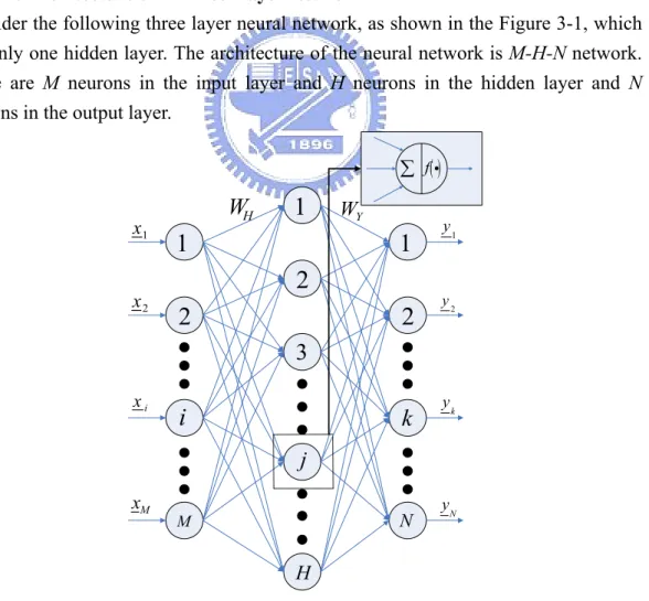
(23) CHAPTER 3 Dynamic Optimal Training of A Three-Layer Neural Network with Sigmoid Function In this chapter, we will try to solve the problem of finding the suitable learning rate for the training of a three layer neural network. For solving this problem, we will find the dynamic optimal learning rate of every iteration. The neural network with one hidden layer is enough to solve the most problems in classification. So the dynamical optimal training algorithm will be proposed in this Chapter for a three layer neural network with sigmoid activation functions in the hidden and output layers in this chapter. 3.1. The Architecture of A Three-Layer Network Consider the following three layer neural network, as shown in the Figure 3-1, which has only one hidden layer. The architecture of the neural network is M-H-N network. There are M neurons in the input layer and H neurons in the hidden layer and N neurons in the output layer. ∑ f ( i) x1. x2. WH. 1. 1. WY. 1. 2 2. 2. y1. y2. 3 xi. i. k. yk. j xM. N. M. yN. H. Figure 3-1. The three layer neural network 14.

(24) There is no activation function in the neurons of the input layer. And the activation function for the neurons in the hidden and output layers is defined by 1 (3.1) f ( x) = 1 + exp(− x) Note that we don’t consider the bias in this chapter. 3.2. The Dynamic Optimal Learning Rate Suppose we are given the following training matrix and the desired output matrix:. X M ×P. ⎡ x11 ⎢x = ⎢ 21 ⎢ ⎢ ⎣⎢ xM 1. ⎡ d11 ⎢d D = ⎢ 21 ⎢ ⎢ ⎢⎣ d N 1. x12 x22 xM 2 d12 d 22 dN 2. x1P ⎤ x2 P ⎥⎥ ⎥ ⎥ xMP ⎦⎥ M ×P. (3.2). d1P ⎤ d 2 P ⎥⎥ ⎥ ⎥ d NP ⎥⎦ N × P. (3.3). There are P columns in (3.2) and (3.3) which implies that there are P sets of training examples. And the weighting matrix between the input layer and the hidden layer is expressed as:. ⎡ w11hidden ⎢ hidden w WH = ⎢ 21 ⎢ ⎢ hidden ⎢⎣ wH 1. ⎤ w1hidden M hidden ⎥ w2 M ⎥ ⎥ hidden ⎥ wHM ⎥⎦ H ×M. w12hidden hidden w22 wHhidden 2. (3.4). The weighting matrix between the hidden layer and the output layer is expressed as:. ⎡ w11 ⎢w WY = ⎢ 21 ⎢ ⎢ ⎢⎣ wN 1. w1H ⎤ w2 H ⎥⎥ ⎥ ⎥ wNH ⎥⎦ N × H. w12 w22 wN 2. (3.5). Then, we can get the linear combiner output of the hidden layer due to (3.2) and (3.4) which is expressed as:. ⎡ s11hidden ⎢ hidden s S H = WH ⋅ X = ⎢ 21 ⎢ ⎢ hidden ⎣⎢ sH 1. s12hidden hidden s22 sHhidden 2 15. ⎤ s1hidden P hidden ⎥ s2 P ⎥ ⎥ hidden ⎥ sHP ⎦⎥ H × P. (3.6).

(25) And by using (3.1) and (3.6), the output matrix of the hidden layer is expressed as below.. ⎡ f ( s11hidden ) v1P ⎤ ⎢ hidden ⎢ f ( s21 v2 p ⎥⎥ ) =⎢ ⎥ ⎢ ⎥ vHP ⎥⎦ H × P ⎢ f s hidden ⎢⎣ ( H 1 ). ⎡ v11 v12 ⎢v v22 V = ⎢ 21 ⎢ ⎢ ⎢⎣vH 1 vH 2. 1 ⎡ hidden ⎢ − s11 + e 1 ⎢ 1 ⎢ hidden ⎢ = 1 + e − s21 ⎢ ⎢ ⎢ 1 ⎢ hidden ⎢⎣1 + e − sH 1. f ( s12hidden ). hidden f ( s22 ). f ( sHhidden ) 2. 1. 1. hidden − s12. − s1hidden P. 1+ e 1. hidden. 1 + e − s22. 1+ e 1. hidden. 1 + e − s2 P. 1 1+ e. − sHhidden 2. f ( s1hidden )⎤⎥ P f ( s2hidden )⎥⎥ P ⎥ hidden ⎥ f ( sHP )⎥⎦ H ×P. 1 hidden. 1 + e − sHP. ⎤ ⎥ ⎥ ⎥ ⎥ ⎥ ⎥ ⎥ ⎥ ⎥⎦ H × P. (3.7). The linear combiner output of the output layer due to (3.5) and (3.7) is expressed as:. ⎡ s11 ⎢s SY = WY ⋅V = ⎢ 21 ⎢ ⎢ ⎢⎣ sN 1. s12 s22 sN 2. s1P ⎤ s2 P ⎥⎥ ⎥ ⎥ sNP ⎥⎦ N ×P. (3.8). And the output of the output layer, which is also the actual output of the network: ⎡ y11 ⎢y Y = ⎢ 21 ⎢ ⎢ ⎢⎣ yN 1. y12 y22 yN 2. ⎡ f ( s11 ) y1P ⎤ ⎢ ⎥ f ( s21 ) y2 P ⎥ =⎢ ⎢ ⎥ ⎢ ⎥ y NP ⎥⎦ N × P ⎢⎣ f ( sN 1 ). ⎡ 1 ⎢ 1 + e − s11 ⎢ ⎢ 1 = ⎢ 1 + e− s21 ⎢ ⎢ ⎢ 1 ⎢ ⎣1 + e − s N 1. f ( s12 ) f ( s22 ) f ( sN 2 ). 1 1 + e− s12 1 1 + e− s22. 1 1 + e − s1 P 1 1 + e − s2 P. 1 1 + e − sN 2. 1 1 + e− sNP. ⎤ ⎥ ⎥ ⎥ ⎥ ⎥ ⎥ ⎥ ⎥ ⎦ N ×P. f ( s1P ) ⎤ ⎥ f ( s2 P ) ⎥ ⎥ ⎥ f ( sNP ) ⎥⎦ N × P. (3.9). Substituting (3.8) into (3.1) then we can get (3.9). The most important parameter of the BP algorithm is the error signal. And the error signal is the difference between the actual output of the network and the desire output. So, we define the error function E as: 16.

(26) ⎡ e11 e12 ⎢e e22 = − = E Y D ⎢ 21 ⎢ ⎢ ⎣⎢ eN 1 eN 2 ⎡ y11 − d11 ⎢ y −d = ⎢ 21 21 ⎢ ⎢ ⎢⎣ yN 1 − d N 1. e1P ⎤ e2 P ⎥⎥ ⎥ ⎥ eNP ⎦⎥ N × P. y12 − d12. y1P − d1P ⎤ y2 P − d 2 P ⎥⎥ ⎥ ⎥ yNP − d NP ⎥⎦ N × P. y22 − d 22 yN 2 − d N 2. (3.10). Finial, we define the total squared error, the energy function of the network, J as follows: 2. J=. 1 P N 1 ykp − d kp ) = Tr ( E T i E ) ( ∑∑ 2 p =1 k =1 2. (3.11). The topic of the learning process is to minimize the total square error J. According to Back-propagation algorithm, we use the method of steepest descent to adjust the synaptic weights. And we apply formula (3.12) and (3.14) to update the weighting matrixes WH and WY. Equation (3.12) and (3.14) are expressed as follow.. ∂J ∂WH. WH ( t + 1) = WH ( t ) − β H. or. whidden ( t + 1) = whidden ( t ) − βY ⋅ ji ji. ∂J ∂whidden ji. (3.12) t. ，. ( j = 1, 2,. , H ；i = 1, 2,. ,M ). t. (3.13). WY ( t + 1) = WY ( t ) − βY. or. wkj ( t + 1) = wkj ( t ) − βY ⋅. ∂J ∂WY. ∂J ∂wkj. (3.14) t. ，. ( k = 1, 2,. , N ；j = 1, 2,. ,H). t. (3.15) Where t denotes the t iteration and βH and βY are the learning rate of WH and WY respectively. Now, let us consider the derivative of (3.15) only, ∂J ∂J ∂yk1 ∂sk1 ∂J ∂yk 2 ∂sk 2 ∂J ∂ykP ∂skP = ⋅ ⋅ + ⋅ ⋅ + + ⋅ ⋅ ∂wkj ∂yk1 ∂sk1 ∂wkj ∂yk 2 ∂sk 2 ∂wkj ∂ykP ∂skP ∂wkj th. 17.

(27) ∂J ∂ykp ∂skp ⋅ ⋅ p =1 ∂ykp ∂skp ∂wkj P. =∑. (3.16). In which, ∂J ∂ = ∂ykp ∂ykp ∂ykp ∂skp. =. 2 ⎡1 P N ⎤ ⎢ ∑∑ ( ykp − d kp ) ⎥ = ( ykp − d kp ) ⎣⎢ 2 p =1 k =1 ⎦⎥. ∂ −s 1 + e kp ∂skp. ∂skp ∂wkj. (. =. ) = (1 + e ) −1. − skp. −2. ∂ ( wk1v1 p + wk 2v2 p + ∂wkj. ⋅e. − skp. (3.17). = ykp (1 − ykp ). (3.18). + wkH vHp ) = v jp. (3.19). Accordingly, the use of (3.17)、(3.18) and (3.19) in (3.16) yields P ∂J = ∑ ( ykp − d kp ) ⋅ ykp (1 − ykp ) ⋅ v jp ∂wkj p =1. (3.20). So, we can rewrite (3.15) as P. wkj ( t + 1) = wkj ( t ) − βY ⋅ ∑ ( ykp − d kp ) ⋅ ykp (1 − ykp ) ⋅ v jp p =1. ( k = 1, 2,. t. , N ；j = 1, 2,. ,H). (3.21). Equation (3.21) is the formula that we use to adjust the synaptic weights WY. Furthermore, let us consider the weighting matrix WH between the input layer and the hidden layer, as expressed in (3.13):. whidden ( t + 1) = whidden ( t ) − βY ⋅ ji ji. ∂J ∂whidden ji. (3.13) t. For the convenience, we just discuss the derivative of (3.13) in the beginning. ∂J ∂J ∂v j1 ∂J ∂v j 2 = + + hidden hidden ∂w ji ∂v j1 ∂w ji ∂v j 2 ∂whidden ji. +. ∂J ∂v jP ∂v jP ∂whidden ji. ⎛ ∂J ∂y11 ∂J ∂y21 =⎜ + + ⎜ ∂y11 ∂v j1 ∂y21 ∂v j1 ⎝. +. ∂J ∂y N 1 ⎞ ∂v j1 + ⎟⋅ ∂y N 1 ∂v j1 ⎟⎠ ∂whidden ji. ⎛ ∂J ∂y12 ∂J ∂y22 + + ⎜⎜ ⎝ ∂y12 ∂v j 2 ∂y22 ∂v j 2. +. ∂J ∂y N 2 ⎞ ∂v j 2 + ⎟⋅ ∂y N 2 ∂v j 2 ⎟⎠ ∂whidden ji. 18.

(28) +. ……… ⎛ ∂J ∂y1P ∂J ∂y2 P + + ⎜⎜ ⎝ ∂y1P ∂v jP ∂y2 P ∂v jP ∂v jp. P. =∑ p =1. p =1. ∂s. ⎛ ∂J ∂ykp ⎝ kp ∂v jp. ∑ ⎜⎜ ∂y. hidden k =1 ji. ∂v jp. P. =∑. ∂w. N. +. ∂s hidden jp ∂w. hidden jp. N. ∂J ∂y NP ∂y NP ∂v jP. ⎞ ⎟⎟ ⎠. ⎛ ∂J ∂ykp ⎝ kp ∂v jp. ∑ ⎜⎜ ∂y. hidden k =1 ji. ⎞ ∂v jP ⎟⎟ ⋅ hidden ⎠ ∂w ji. ⎞ ⎟⎟ ⎠. (3.22). In which, ∂ykp ∂v jp. =. ∂ykp ∂skp ∂skp ∂v jp. = ykp (1 − ykp ) ⋅ wkj. (3.23). In which we substitute (3.18) into (3.23). ∂v jp ∂s. hidden jp. ∂s hidden jp ∂w. hidden ji. =. =. ∂ ∂s. ∂ ∂w. (1 + e ) = (1 + e ) −1. − s hidden jp. hidden jp. hidden ji. (w. − s hidden jp. x + whidden x2 p + j2. hidden j1 1p. −2. e. − s hidden jp. = v jp (1 − v jp ). (3.24). xMp ) = x jp + whidden jM. (3.25). Accordingly, the use of (3.17)、(3.23)、(3.24) and (3.25) in (3.22) yields P N ∂J ⎡ 1 = v − v ⋅ x ⋅ ( ) ∑ jp ip ∑ ⎢ jp ∂whidden p =1 ⎣ k =1 ji. (( y. kp. ⎤ − d kp ) ⋅ ykp (1 − ykp ) ⋅ wkj ⎥ ⎦. ). (3.26). So, we can rewrite (3.13) as N ⎧P ⎡ ⎤⎫ hidden whidden t 1 w t β v 1 v x + = − ⋅ − ⋅ ⋅ ( ) ( ) ( ) ⎨ ∑ ji ji H jp ip ∑ ( ykp − d kp ) ⋅ ykp (1 − ykp ) ⋅ wkj ⎥ ⎬ ⎢ jp k =1 ⎦⎭ ⎩ p =1 ⎣. (. ，. ( j = 1, 2,. , H ；i = 1, 2,. ,M ). ). (3.27). Equation (3.27) is the formula that we use to adjust the synaptic weights WH. By using (3.21) and (3.27), we can adjust the synaptic weights of the network. 3.3. Dynamical Optimal Training via Lyapunov’s Method In control system, we know that we can use the Lyapunov function to consider the stability of the system. The basic philosophy of Lyapunov’s direct method is the mathematical extension of a fundamental physical observation: if the total energy of a 19.

(29) mechanical (or electrical) system is continuously dissipated, then the system, whether linear or nonlinear must eventually settle down to an equilibrium point [19]. So by the same meaning, we define the Lyapunov function as V =J (3.28) Where the item J is total square error, defined in (3.11). And Equation (3.28) is positive definite, which means that V = J > 0. The difference of the Lyapunov function is ∆V = J t +1 − J t (3.29) Where Jt+1 expresses the total square error of the (t+1)th iteration. If Equation (3.29) is negative, the system is guaranteed to be stable. Then, for △V < 0 we have J t +1 − J t < 0 (3.30) So, by using (3.11) we can get 2. J t +1 − J t =. =. 1 P N 1 P N 1 y t + − d − ( ) ( ) ∑∑ kp ∑∑ ( ykp ( t ) − d kp ) kp 2 p =1 k =1 2 p =1 k =1. 2. 2 2 1 P N ⎡ ⎤ + − − − y t d y t d 1 ( ) ( ) ( ) ( ) ∑∑ kp kp kp kp ⎦⎥ 2 p =1 k =1 ⎣⎢. = G ( β H ( t ) , βY ( t ) ). (3.31). In Equation (3.31), the item Jt is already known and the Jt+1 is the function of βH(t) and βY(t), so Jt+1-Jt can be expressed as a new function G of βH(t) and βY(t). For simplification, we can assume that βH(t) = βY(t) = β(t), then the function G only has one parameter G(β(t)). The Equation (3.31) can be rewritten as. J t +1 − J t = G ( β ( t ) ). (3.32). If the parameter β(t) satisfies Jt+1 - Jt = G(β(t)) <0, then the set of β(t) is the stable range of the learning rate of the system at the tth iteration. In this stable range, if the βopt(t) satisfies that Jt+1 - Jt is at its minimum, we call βopt(t) the optimal learning rate at the tth iteration. The optimal learning rate βopt(t) will not only guarantee the stability of the training process, but also has the fastest speed of convergence. In order to find the optimal learning rate βopt(t) from the function Jt+1 - Jt analytically, we need to have an explicit form of Jt+1 - Jt, like the simplest form of Jt+1 - Jt (for a simple two layer neural network) in [13]. But the function Jt+1 - Jt here is a very complicated nonlinear algebraic equation, it is nearly impossible to have a simple explicit form. However we have also defined the function Jt+1 - Jt in (3.31) by progressively evolving the equations from the beginning of this Chapter. Therefore we can indeed defined (3.31) implicitly in Matlab coding. In this case, we can apply the Matlab routine fminbnd to find the optimal learning rate βopt(t) from Jt+1 - Jt. The 20.

(30) calling sequence of fminbnd is: FMINBND Scalar bounded nonlinear function minimization. X = FMINBND(FUN,x1,x2) starts at X0 and finds a local minimizer X of the function FUN in the interval x1 <= X <= x2. FUN accepts scalar input X and returns a scalar function value F evaluated at X. The capability of the Matlab routine “fminbnd” is to find a local minimizer βopt of the function G(β), which has only one independent variable β, in a given interval. So we have to define an interval when we use this routine. For the following two examples in Chapter 4, we set the interval as [0.01, 100] to set the allowable learning rates between 0.01 and 100. Note that for simplicity, we assume that βH(t) = βY(t) = β(t) in (3.31), therefore there is only one variable in (3.31). So we use the routine “fminbnd” to find the optimal learning rate. However, we can also find the learning rate βH(t) and. βY(t) respectively by using another Matlab routine “fminunc”. But this routine “fminunc” can only find the minimizer βH(t) and βY(t) around one specific point, not around an interval. Therefore it is very limited in application and is not appropriate for this case. Algorithm 1: Dynamic optimal training algorithm for a three-layer neural network Step 0: The following WH(t), WY(t), G(β(t)), βopt(t) and Y(t) denote their respective values at iteration t. Step 1: Given the initial weighting matrix WH(1), WY(1), the training input matrix X and the desired output matrix D then we can find the actual output matrix of the network Y(1) and the nonlinear function G(β(1)). Step 2: Using Matlab routine “fminbnd” with the interval [0.01, 100] to solve the nonlinear function G(β(1)) and find the optimal learning rate βopt(1). Step 3: Iteration count t=1. Start the back propagation training process. Step 4: Find if the desired output matrix D and the actual output matrix of the network Y(1) are close enough or not? If Yes, GOTO Step 9. Step 5: Update the synaptic weights matrix to yield WH(t+1) and WY(t+1) by using (3.27) and (3.21) respectively. Step 6: Find the actual output matrix of the network Y(t+1) and the nonlinear function G(β(t+1)). Step 7: Use Matlab routine “fminbnd” to find the optimal learning rate βopt(t+1) for the next iteration. Step 8: t=t+1 and GOTO Step 4. Step 9: End. 21.

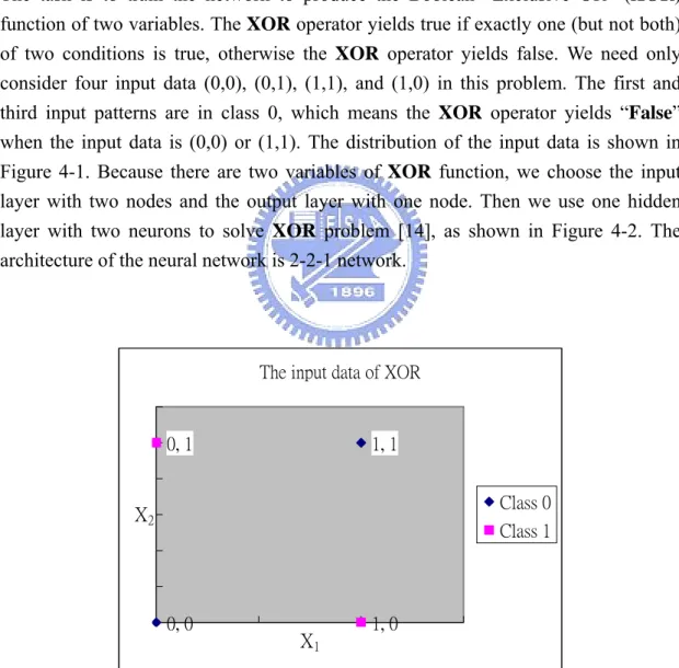
(31) CHAPTER 4 Experimental Results In this chapter, the classification problems of XOR and Iris data will be solved via our new dynamical optimal training algorithm in Chapter 3. The training results will be compared with the conventional BP training using fixed learning rate. 4.1. Example 1: The XOR Problem The task is to train the network to produce the Boolean “Exclusive OR” (XOR) function of two variables. The XOR operator yields true if exactly one (but not both) of two conditions is true, otherwise the XOR operator yields false. We need only consider four input data (0,0), (0,1), (1,1), and (1,0) in this problem. The first and third input patterns are in class 0, which means the XOR operator yields “False” when the input data is (0,0) or (1,1). The distribution of the input data is shown in Figure 4-1. Because there are two variables of XOR function, we choose the input layer with two nodes and the output layer with one node. Then we use one hidden layer with two neurons to solve XOR problem [14], as shown in Figure 4-2. The architecture of the neural network is 2-2-1 network.. The input data of XOR. 0, 1. 1, 1 Class 0. X2. Class 1. 0, 0. 1, 0. X1. Figure 4-1. The distribution of XOR input data sets. 22.

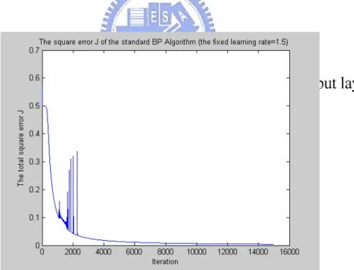
(32) x1. W1 W5. W2. y. W3. W6. x2. W4. Figure 4-2. The neural network for solving XOR First, we use the standard BP algorithm with fixed learning rates (β = 1.5, 0.9, 0.5 and 0.1) to train the XOR, and the training results are shown in Figure 4-3-1 ~ 4-3-4. The result of using BP algorithm with dynamic optimal learning rates to train the XOR is shown Figure 4-4.. Figure 4-3-1. The square error J of the standard BPA with fixed β = 1.5. 23.

(33) Figure 4-3-2. The square error J of the standard BPA with fixed β = 0.9. Figure 4-3-3. The square error J of the standard BPA with fixed β = 0.5. 24.

(34) Figure 4-3-4. The square error J of the standard BPA with fixed β = 0.1. Figure 4-4. The square error J of the BPA with dynamic optimal training. The following Figure 4-5 shows the plot of (3.32) for -1 < β < 100, which is G(β) = ∆J(β) = Jt+1 - Jt, at iteration count t = 1. The Matlab routine fminbnd will be invoked to find βopt with the constraint that G(βopt) < 0 with maximum absolute value. This βopt is the learning rate for iteration count t = 2.The βopt is found to be 7.2572 for iteration count 2. The dynamic learning rate of every iteration is shown in Figure 4-6. 25.

(35) Figure 4-5. The difference equation G(β(n)) and βopt = 7.2572. Figure 4-6. The dynamic learning rates of every iteration. 26.

(36) The comparison of these cases is shown in Figure 4-7. In Figure 4-7, it is obvious that our dynamical optimal training yields the best training results in minimum epochs.. Figure 4-7. Training errors of dynamic optimal learning rates and fixed learning rates. Table 4-1 shows the training result via dynamical optimal training for XOR problem. Table 4.1. The training result for XOR using dynamical optimal training Iterations. 1000. 5000. 10000. 15000. W1 (after trained). 6.5500. 7.7097. 8.8191. 8.4681. W2 (after trained). 6.5652. 7.7145. 8.1921. 8.4703. W3 (after trained). 0.8591. 0.9265. 0.9473. 0.9573. W4 (after trained). 0.8592. 0.9265. 0.9473. 0.9573. W5 (after trained). 14.9536. 26.2062. 33.0393. 37.8155. W6 (after trained). -19.0670. -32.9550. -41.3692. -47.2513. Actual Output Y for (x1, x2) = (0,0). 0.1134. 0.0331. 0.0153. 0.0089. Actual Output Y for (x1, x2) = (0,1). 0.8232. 0.9300. 0.9616. 0.9750. Actual Output Y for (x1, x2) = (1,0). 0.8232. 0.9300. 0.9616. 0.9750. Actual Output Y for (x1, x2) = (1,1). 0.2291. 0.0925. 0.0511. 0.0334. J. 0.0639. 0.0097. 0.0029. 0.0012. Training Results. 27.

(37) Table 4-2 shows the training result via the standard BP with fixed β = 0.9 for XOR problem. Table 4.2. The training result for XOR using fixed learning rate β = 0.9 Iterations Training Results. 1000. 5000. 10000. 15000. W1 (after trained). 4.7659. 7.2154. 7.6576. 7.8631. W2 (after trained). 4.8474. 7.2228. 7.6624. 7.8670. W3 (after trained). 0.7199. 0.8996. 0.9234. 0.9331. W4 (after trained). 0.7228. 0.8996. 0.9234. 0.9331. W5 (after trained). 6.2435. 20.6467. 25.5617. 28.2288. W6 (after trained). -8.1214. -26.1034. -32.1610. -35.4456. Actual Output Y for (x1, x2) = (0,0). 0.2811. 0.0613. 0.0356. 0.0264. Actual Output Y for (x1, x2) = (0,1). 0.6742. 0.8885. 0.9263. 0.9415. Actual Output Y for (x1, x2) = (1,0). 0.6745. 0.8885. 0.9263. 0.9415. Actual Output Y for (x1, x2) = (1,1). 0.4192. 0.1479. 0.0982. 0.0781. J. 0.2334. 0.0252. 0.0109. 0.0068. To compare Table 4.1 with Table 4.2, we can see that the training result via dynamical optimal training is faster with better result than other approaches. Now, we will use another method, the back-propagation algorithm with momentum, to solve XOR problem again. Then we will compare its training errors with that of dynamic optimal training and see if dynamic optimal training is indeed better. The back-propagation algorithm with momentum is to modify the Equation (2.13) by including a momentum term as follows: ∂J ∆W ( t ) = −η + α ⋅ ∆W ( t − 1) (4.1) ∂W t where α is usually a positive number called the momentum constant and usually in the range [0, 1). The training results of the BPA with momentum for XOR problem are shown in Figure 4-8-1 ~ 4-8-3. The comparison of these cases is shown in Figure 4-9. In Figure 4-9, we can see that some training results of BPA with momentum are as well as the dynamic training but the most results of BPA with momentum are unpredictable. The training results still depend on the chosen learning rates and momentum.. 28.

(38) Figure 4-8-1. The square error J of the BPA with variant momentum(β = 0.9). Figure 4-8-2. The square error J of the BPA with variant momentum(β = 0.5). 29.

(39) Figure 4-8-3. The square error J of the BPA with variant momentum (β = 0.1). Figure 4-9. Total square errors of dynamic training and the BPA with different learning rates and momentum. 30.

(40) 4.2. Example 2: Classification of Iris Data Set In this example, we will use the same neural network as before to classify Iris data sets [15], [16]. Generally, Iris has three kinds of subspecies, and the classification will depend on the length and width of the petal and the length and width of the sepal. The total Iris data are shown in Figure 4-10-1 and 4-10-2. And the training data sets, the first 75 samples of total data, are shown in Figures 4-11-1 and 4-11-2. The Iris data samples are available in [20]. There are 150 samples of three species of the Iris flowers in this data. We choose 75 samples to train the network and using the other 75 samples to test the network. We will have four kinds of input data, so we adopt the network which has four nodes in the input layer and three nodes in the output layer for this problem. Then the architecture of the neural network is a 4-4-3 network as shown in Figure 4-12. In which, we use the network with four hidden nodes in the hidden layer.. IRIS Data-Sepal. Sepal width (in cm). Class 1-setosa. Class 2-versicolor. Class 3-virginica. 5 4.5 4 3.5 3 2.5 2 1.5 1 4. 5. 6. 7. Sepal length (in cm). Figure 4-10-1. The total Iris data set (Sepal). 31. 8.

(41) IRIS Data-Petal Class 1-setosa. Class 2-versicolor. Class 3-virginica. 3 Petal width (in cm). 2.5 2 1.5 1 0.5 0 0. 2. 4. 6. 8. Petal length (in cm) Figure 4-10-2. The total Iris data set (Petal). IRIS Data-Sepal Class 1-setosa. Class 2-versicolor. Class 3-virginica. 5. Sepal width (in cm). 4.5 4 3.5 3 2.5 2 1.5 1 4. 5. 6. 7. Sepal length (in cm). Figure 4-11-1. The training set of Iris data (Sepal). 32. 8.

(42) IRIS Data-Petal Class 1-setosa. Class 2-versicolor. Class 3-virginica. Petal width (in cm. 3 2.5 2 1.5 1 0.5 0 0. 2. 4. 6. 8. Petal length (in cm). Figure 4-11-2. The training set of Iris data (Petal). x1. WH. WY y1. x2. y2 x3. y3 x4. Figure 4-12. The neural network for solving Iris problem First, we use the standard BPA with fixed learning rates (β = 0.1, 0.01 and 0.001) to solve the classification of Iris data sets, and the training results are shown in Figure 4-13-1 ~ 4-13-3. The result of BPA with dynamic optimal learning rates is shown in Figure 4-14. 33.

(43) Figure 4-13-1. The square error J of the standard BPA with fixed β = 0.1. Figure 4-13-2. The square error J of the standard BPA with fixed β = 0.01. 34.

(44) Figure 4-13-3. The square error J of the standard BPA with fixed β = 0.001. Figure 4-14. The square error J of the BPA with dynamic optimal training. 35.

(45) Figure 4-15 shows that the convergence speed of the network with dynamic learning rate is absolutely faster than the network with fixed learning rates. Because the optimal learning rate of every iteration is almost in the range [0.01, 0.02], so the convergence speed of the fixed learning rate β = 0.01 is similar to the convergence speed of the dynamic learning rate. But dynamic learning rate approach still performs better than those of using fixed learning rates.. Figure 4-15. Training errors of dynamic optimal learning rates and fixed learning rates After 10000 training iterations, the resulting weights and total square error J are shown below.. ⎡ 1.2337 -0.5033 1.3225 1.3074 ⎤ ⎢-0.3751 3.4714 -2.6777 -1.6052 ⎥ ⎥ WH = ⎢ ⎢ 3.7235 5.1603 -4.0019 -10.4289 ⎥ ⎢ ⎥ ⎣ 1.9876 -2.7186 4.6171 4.3400 ⎦. ⎡-2.2947 7.8444 3.4765 -5.0185⎤ WY = ⎢⎢ -2.5365 -8.5464 9.3797 -2.1300 ⎥⎥ ⎢⎣ 2.0822 -3.7674 -10.4114 3.0220 ⎥⎦ Total square error J = 0.1582. 36.

(46) The actual output and desired output of 10000 training iteration are shown in Table 4.3 and the testing output and desired output are shown in Table 4.4. After we substitute the above weighting matrices into the network and perform real testing, we find that there is no classification error by using training set (the first 75 data set). However there are 5 classification errors by using testing set (the later 75 data set), which are index 34, 51, 55, 57, 59 in Table 4-4. Table 4.3. Actual and desired outputs after 10000 iterations Actual Output Index. Desired Output. Class 1. Class 2. Class 3. Class 1. Class 2. Class 3. 1. 0.9819. 0.0216. 0.0001. 1.0000. 0.0000. 0.0000. 2. 0.9807. 0.0233. 0.0001. 1.0000. 0.0000. 0.0000. 3. 0.9817. 0.0220. 0.0001. 1.0000. 0.0000. 0.0000. 4. 0.9810. 0.0229. 0.0001. 1.0000. 0.0000. 0.0000. 5. 0.9821. 0.0215. 0.0001. 1.0000. 0.0000. 0.0000. 6. 0.9819. 0.0215. 0.0001. 1.0000. 0.0000. 0.0000. 7. 0.9819. 0.0218. 0.0001. 1.0000. 0.0000. 0.0000. 8. 0.9817. 0.0219. 0.0001. 1.0000. 0.0000. 0.0000. 9. 0.9804. 0.0237. 0.0001. 1.0000. 0.0000. 0.0000. 10. 0.9810. 0.0228. 0.0001. 1.0000. 0.0000. 0.0000. 11. 0.9820. 0.0215. 0.0001. 1.0000. 0.0000. 0.0000. 12. 0.9816. 0.0221. 0.0001. 1.0000. 0.0000. 0.0000. 13. 0.9810. 0.0229. 0.0001. 1.0000. 0.0000. 0.0000. 14. 0.9821. 0.0222. 0.0001. 1.0000. 0.0000. 0.0000. 15. 0.9822. 0.0213. 0.0001. 1.0000. 0.0000. 0.0000. 16. 0.9822. 0.0213. 0.0001. 1.0000. 0.0000. 0.0000. 17. 0.9821. 0.0214. 0.0001. 1.0000. 0.0000. 0.0000. 18. 0.9819. 0.0217. 0.0001. 1.0000. 0.0000. 0.0000. 19. 0.9818. 0.0216. 0.0001. 1.0000. 0.0000. 0.0000. 20. 0.9821. 0.0215. 0.0001. 1.0000. 0.0000. 0.0000. 21. 0.9811. 0.0226. 0.0001. 1.0000. 0.0000. 0.0000. 22. 0.9819. 0.0216. 0.0001. 1.0000. 0.0000. 0.0000. 23. 0.9829. 0.0218. 0.0001. 1.0000. 0.0000. 0.0000. 24. 0.9800. 0.0240. 0.0001. 1.0000. 0.0000. 0.0000. 25. 0.9808. 0.0231. 0.0001. 1.0000. 0.0000. 0.0000. 26. 0.0214. 0.9910. 0.0049. 0.0000. 1.0000. 0.0000. 27. 0.0215. 0.9908. 0.0049. 0.0000. 1.0000. 0.0000. 37.

(47) 28. 0.0211. 0.9909. 0.0050. 0.0000. 1.0000. 0.0000. 29. 0.0174. 0.9846. 0.0090. 0.0000. 1.0000. 0.0000. 30. 0.0205. 0.9902. 0.0055. 0.0000. 1.0000. 0.0000. 31. 0.0202. 0.9895. 0.0058. 0.0000. 1.0000. 0.0000. 32. 0.0210. 0.9903. 0.0052. 0.0000. 1.0000. 0.0000. 33. 0.0243. 0.9895. 0.0046. 0.0000. 1.0000. 0.0000. 34. 0.0213. 0.9910. 0.0049. 0.0000. 1.0000. 0.0000. 35. 0.0189. 0.9861. 0.0076. 0.0000. 1.0000. 0.0000. 36. 0.0208. 0.9899. 0.0055. 0.0000. 1.0000. 0.0000. 37. 0.0213. 0.9902. 0.0052. 0.0000. 1.0000. 0.0000. 38. 0.0212. 0.9910. 0.0049. 0.0000. 1.0000. 0.0000. 39. 0.0203. 0.9898. 0.0057. 0.0000. 1.0000. 0.0000. 40. 0.0251. 0.9892. 0.0045. 0.0000. 1.0000. 0.0000. 41. 0.0216. 0.9909. 0.0049. 0.0000. 1.0000. 0.0000. 42. 0.0172. 0.9836. 0.0095. 0.0000. 1.0000. 0.0000. 43. 0.0218. 0.9907. 0.0049. 0.0000. 1.0000. 0.0000. 44. 0.0072. 0.8555. 0.1140. 0.0000. 1.0000. 0.0000. 45. 0.0216. 0.9907. 0.0049. 0.0000. 1.0000. 0.0000. 46. 0.0058. 0.7622. 0.2006. 0.0000. 1.0000. 0.0000. 47. 0.0218. 0.9907. 0.0049. 0.0000. 1.0000. 0.0000. 48. 0.0090. 0.9154. 0.0618. 0.0000. 1.0000. 0.0000. 49. 0.0210. 0.9908. 0.0051. 0.0000. 1.0000. 0.0000. 50. 0.0215. 0.9909. 0.0049. 0.0000. 1.0000. 0.0000. 51. 0.0007. 0.0093. 0.9940. 0.0000. 0.0000. 1.0000. 52. 0.0007. 0.0101. 0.9934. 0.0000. 0.0000. 1.0000. 53. 0.0007. 0.0119. 0.9920. 0.0000. 0.0000. 1.0000. 54. 0.0008. 0.0162. 0.9888. 0.0000. 0.0000. 1.0000. 55. 0.0007. 0.0095. 0.9939. 0.0000. 0.0000. 1.0000. 56. 0.0007. 0.0103. 0.9933. 0.0000. 0.0000. 1.0000. 57. 0.0007. 0.0102. 0.9933. 0.0000. 0.0000. 1.0000. 58. 0.0011. 0.0330. 0.9752. 0.0000. 0.0000. 1.0000. 59. 0.0007. 0.0108. 0.9929. 0.0000. 0.0000. 1.0000. 60. 0.0007. 0.0099. 0.9936. 0.0000. 0.0000. 1.0000. 61. 0.0024. 0.2245. 0.7853. 0.0000. 0.0000. 1.0000. 62. 0.0008. 0.0131. 0.9912. 0.0000. 0.0000. 1.0000. 63. 0.0008. 0.0138. 0.9906. 0.0000. 0.0000. 1.0000. 64. 0.0007. 0.0094. 0.9939. 0.0000. 0.0000. 1.0000. 38.

(48) 65. 0.0007. 0.0093. 0.9940. 0.0000. 0.0000. 1.0000. 66. 0.0007. 0.0100. 0.9935. 0.0000. 0.0000. 1.0000. 67. 0.0016. 0.0894. 0.9242. 0.0000. 0.0000. 1.0000. 68. 0.0013. 0.0511. 0.9596. 0.0000. 0.0000. 1.0000. 69. 0.0007. 0.0093. 0.9940. 0.0000. 0.0000. 1.0000. 70. 0.0010. 0.0291. 0.9785. 0.0000. 0.0000. 1.0000. 71. 0.0007. 0.0102. 0.9933. 0.0000. 0.0000. 1.0000. 72. 0.0007. 0.0098. 0.9936. 0.0000. 0.0000. 1.0000. 73. 0.0007. 0.0103. 0.9933. 0.0000. 0.0000. 1.0000. 74. 0.0017. 0.1066. 0.9075. 0.0000. 0.0000. 1.0000. 75. 0.0008. 0.0164. 0.9887. 0.0000. 0.0000. 1.0000. Table 4.4. Actual and desired outputs in real testings Actual Output. Desired Output. Index. Class 1. Class 2. Class 3. Class 1. Class 2. Class 3. 1. 0.9794. 0.0249. 0.0001. 1.0000. 0.0000. 0.0000. 2. 0.9812. 0.0224. 0.0001. 1.0000. 0.0000. 0.0000. 3. 0.9818. 0.0218. 0.0001. 1.0000. 0.0000. 0.0000. 4. 0.9818. 0.0218. 0.0001. 1.0000. 0.0000. 0.0000. 5. 0.9810. 0.0229. 0.0001. 1.0000. 0.0000. 0.0000. 6. 0.9804. 0.0236. 0.0001. 1.0000. 0.0000. 0.0000. 7. 0.9813. 0.0223. 0.0001. 1.0000. 0.0000. 0.0000. 8. 0.9823. 0.0214. 0.0001. 1.0000. 0.0000. 0.0000. 9. 0.9823. 0.0213. 0.0001. 1.0000. 0.0000. 0.0000. 10. 0.9810. 0.0228. 0.0001. 1.0000. 0.0000. 0.0000. 11. 0.9818. 0.0219. 0.0001. 1.0000. 0.0000. 0.0000. 12. 0.9820. 0.0216. 0.0001. 1.0000. 0.0000. 0.0000. 13. 0.9810. 0.0228. 0.0001. 1.0000. 0.0000. 0.0000. 14. 0.9813. 0.0226. 0.0001. 1.0000. 0.0000. 0.0000. 15. 0.9817. 0.0219. 0.0001. 1.0000. 0.0000. 0.0000. 16. 0.9820. 0.0216. 0.0001. 1.0000. 0.0000. 0.0000. 17. 0.9650. 0.0442. 0.0002. 1.0000. 0.0000. 0.0000. 18. 0.9819. 0.0220. 0.0001. 1.0000. 0.0000. 0.0000. 19. 0.9813. 0.0224. 0.0001. 1.0000. 0.0000. 0.0000. 20. 0.9816. 0.0219. 0.0001. 1.0000. 0.0000. 0.0000. 21. 0.9804. 0.0236. 0.0001. 1.0000. 0.0000. 0.0000. 39.

(49) 22. 0.9820. 0.0215. 0.0001. 1.0000. 0.0000. 0.0000. 23. 0.9816. 0.0222. 0.0001. 1.0000. 0.0000. 0.0000. 24. 0.9820. 0.0215. 0.0001. 1.0000. 0.0000. 0.0000. 25. 0.9817. 0.0220. 0.0001. 1.0000. 0.0000. 0.0000. 26. 0.0215. 0.9909. 0.0049. 0.0000. 1.0000. 0.0000. 27. 0.0210. 0.9909. 0.0051. 0.0000. 1.0000. 0.0000. 28. 0.0170. 0.9839. 0.0095. 0.0000. 1.0000. 0.0000. 29. 0.0196. 0.9886. 0.0064. 0.0000. 1.0000. 0.0000. 30. 0.0239. 0.9898. 0.0046. 0.0000. 1.0000. 0.0000. 31. 0.0215. 0.9907. 0.0050. 0.0000. 1.0000. 0.0000. 32. 0.0219. 0.9907. 0.0049. 0.0000. 1.0000. 0.0000. 33. 0.0220. 0.9906. 0.0049. 0.0000. 1.0000. 0.0000. *34. 0.0019. 0.1415. 0.8726. 0.0000. 1.0000. 0.0000. 35. 0.0140. 0.9710. 0.0179. 0.0000. 1.0000. 0.0000. 36. 0.0217. 0.9901. 0.0051. 0.0000. 1.0000. 0.0000. 37. 0.0212. 0.9909. 0.0050. 0.0000. 1.0000. 0.0000. 38. 0.0201. 0.9897. 0.0058. 0.0000. 1.0000. 0.0000. 39. 0.0224. 0.9903. 0.0049. 0.0000. 1.0000. 0.0000. 40. 0.0199. 0.9889. 0.0061. 0.0000. 1.0000. 0.0000. 41. 0.0197. 0.9889. 0.0062. 0.0000. 1.0000. 0.0000. 42. 0.0210. 0.9905. 0.0052. 0.0000. 1.0000. 0.0000. 43. 0.0215. 0.9907. 0.0050. 0.0000. 1.0000. 0.0000. 44. 0.0232. 0.9900. 0.0047. 0.0000. 1.0000. 0.0000. 45. 0.0206. 0.9899. 0.0055. 0.0000. 1.0000. 0.0000. 46. 0.0223. 0.9905. 0.0048. 0.0000. 1.0000. 0.0000. 47. 0.0216. 0.9905. 0.0050. 0.0000. 1.0000. 0.0000. 48. 0.0215. 0.9908. 0.0049. 0.0000. 1.0000. 0.0000. 49. 0.0300. 0.9869. 0.0042. 0.0000. 1.0000. 0.0000. 50. 0.0215. 0.9905. 0.0050. 0.0000. 1.0000. 0.0000. *51. 0.0060. 0.7787. 0.1866. 0.0000. 0.0000. 1.0000. 52. 0.0026. 0.2674. 0.7388. 0.0000. 0.0000. 1.0000. 53. 0.0032. 0.3974. 0.5942. 0.0000. 0.0000. 1.0000. 54. 0.0007. 0.0095. 0.9938. 0.0000. 0.0000. 1.0000. *55. 0.0159. 0.9807. 0.0117. 0.0000. 0.0000. 1.0000. 56. 0.0009. 0.0230. 0.9835. 0.0000. 0.0000. 1.0000. *57. 0.0165. 0.9827. 0.0104. 0.0000. 0.0000. 1.0000. 58. 0.0007. 0.0094. 0.9939. 0.0000. 0.0000. 1.0000. 40.

(50) *59. 0.0133. 0.9690. 0.0199. 0.0000. 0.0000. 1.0000. 60. 0.0018. 0.1281. 0.8862. 0.0000. 0.0000. 1.0000. 61. 0.0007. 0.0106. 0.9930. 0.0000. 0.0000. 1.0000. 62. 0.0007. 0.0095. 0.9939. 0.0000. 0.0000. 1.0000. 63. 0.0018. 0.1130. 0.9011. 0.0000. 0.0000. 1.0000. 64. 0.0033. 0.4128. 0.5766. 0.0000. 0.0000. 1.0000. 65. 0.0011. 0.0335. 0.9748. 0.0000. 0.0000. 1.0000. 66. 0.0007. 0.0094. 0.9939. 0.0000. 0.0000. 1.0000. 67. 0.0008. 0.0166. 0.9885. 0.0000. 0.0000. 1.0000. 68. 0.0007. 0.0101. 0.9934. 0.0000. 0.0000. 1.0000. 69. 0.0007. 0.0096. 0.9938. 0.0000. 0.0000. 1.0000. 70. 0.0007. 0.0094. 0.9939. 0.0000. 0.0000. 1.0000. 71. 0.0007. 0.0105. 0.9931. 0.0000. 0.0000. 1.0000. 72. 0.0007. 0.0123. 0.9917. 0.0000. 0.0000. 1.0000. 73. 0.0010. 0.0284. 0.9791. 0.0000. 0.0000. 1.0000. 74. 0.0007. 0.0099. 0.9935. 0.0000. 0.0000. 1.0000. 75. 0.0011. 0.0370. 0.9717. 0.0000. 0.0000. 1.0000. 41.

(51) CHAPTER 5 Conclusions Although the back propagation algorithm is a useful tool to solve the problems of classification, optimization, prediction etc, it still has many defects. One of those defects is that we don’t know how to choose the suitable learning rate to get converged training results. But by using the dynamical training algorithm for three layer neural network that we proposed in the end of Chapter 3, we can find the dynamic optimal learning rate very easily. And the dynamic learning rate guarantees that the total square error J is a decreasing function. This means that actual outputs will be closer to desired outputs for more iterations. The classification problems of XOR and Iris data are proposed in Chapter 4. They are solved by using the dynamical optimal training for a three layer neural network with sigmoid activation functions in hidden and output layers. Excellent results are obtained in the XOR and Iris data problems. Therefore the dynamic training algorithm is actually very powerful for getting better results than the other conventional back propagation algorithm with unknown fixed learning rates. So the goal of removing the defects of the back propagation algorithm with fixed learning rate is achieved by using the dynamical optimal training algorithm.. 42.

(52) REFERENCES [1] T. Yoshida, and S. Omatu, “Neural network approach to land cover mapping,” IEEE Trans. Geoscience and Remote, Vol. 32, pp. 1103-1109, Sept. 1994. [2] H. Bischof, W. Schneider, and A. J. Pinz, “Multispectral classification of Landsat-images using neural networks,” IEEE Trans, Gsoscience and Remote Sensing, Vol. 30, pp. 482-490, May 1992. [3] M. Gopal, L. Behera, and S. Choudhury, “On adaptive trajectory tracking of a robot manipulator using inversion of its neural emulator,” IEEE Trans. Neural Networks, 1996. [4] L. Behera, “Query based model learning and stable tracking of a roboot arm using radial basis function network,” Elsevier Science LTd., Computers and Electrical Engineering, 2003. [5] F. Amini, H. M. Chen, G. Z. Qi, and J. C. S. Yang, “Generalized neural network based model for structural dynamic identification, analytical and experimental studies,” Intelligent Information Systems, Proceedings 8-10, pp. 138-142, Dec. 1997. [6] K. S. Narendra, and S. Mukhopadhyay, “Intelligent control using neural networks,” IEEE Trans., Control Systems Magazine, Vol. 12, Issue 2, pp.11-18, April 1992. [7] L. Yinghua, and G. A. Cunningham, “A new approach to fuzzy-neural system modeling,” IEEE Trans., Fuzzy Systems, Vol. 3, pp. 190-198, May 1995. [8] L. J. Zhang, and W. B. Wang, “Scattering signal extracting using system modeling method based on a back propagation neural network,” Antennas and Propagation Society International Symposium, 1992. AP-S, 1992 Digest. Held in Conjuction with: URSI Radio Science Meting and Nuclear EMP Meeting, IEEE 18-25, Vol. 4, pp. 2272, July 1992 [9] P. Poddar, and K. P. Unnikrishnan, “Nonlinear prediction of speech signals using memory neuron networks,” Neural Networks for Signal Processing [1991], Proceedings of the 1991 IEEE Workshop 30, pp. 395-404, Oct. 1991. [10] R. P. Lippmann, “An introduction to computing with neural networks,” IEEE ASSP Magazine, 1987. [11] D. E. Rumelhart et al., Learning representations by back propagating error,” Nature, Vol. 323, pp. 533-536, 1986 [12] D. E. Rumelhart, G. E. Hinton, and R. J. Williams, “Learning internal representations by error propagation,” Parallel Distributed Processing, Exploration in the Microstructure of Cognition, Vol. 1, D. E. Rumelhart and J. L. 43.

(53) [13]. [14]. [15]. [16]. [17] [18] [19] [20]. McClelland, eds. Cambridge, MA: MIT Press, 1986. C. H. Wang, H. L. Liu, and C. T. Lin, “Dynamic Optimal Learning Rates of a Certain Class of Fuzzy Neural Networks and its Applications with Genetic Algorithm,” IEEE Trans. Syst., Man, Cybern. Part B, Vol. 31, pp. 467-475, June 2001. L. Behera, S. Kumar, and A. Patnaik, “A novel learning algorithm for feedforeward networks using Lyapunov function approach,” Intelligent Sensing and Information Processing, Proceedings of international Conference, pp. 277-282, 2004. M. A. AL-Alaoui, R. Mouci, M. M. Mansour, and R. Ferzli, “A Cloning Approach to Classifier Training,” IEEE Trans. Syst., Man, Cybern. Part A, Vol. 32, pp. 746-752, Nov. 2002. R. Kozma, M. Kitamura, A. Malinowski, and J. M. Zurada, “On performance measures of artificial neural networks trained by structural learning algorithms,”. Artificial Neural Networks and Expert Systmes, Proceedings, Second New Zealand International Two-Stream Conference, pp.22-25, Nov. 20-23, 1995. F. Rosenblatt, “Principles of Neurodynamics”, Spartan books, New York, 1962. S. Haykin, “Neural Networks: A Comprehensive Foundation,” New Jersey: Prentice-Hall, second edition, 1999. J. E. Slotine, “Applied Nonlinear Control,” New Jersey: Prentice-Hall, 1991. Iris Data Samples [Online]. Available: ftp.ics.uci.edu/pub/machine-learning databases/iris/iris.data.. 44.

(54)