A two-reservoir model to simulate the air discharged from a pulse-jet cleaning system

On: 01 May 2014, At: 01:22

Publisher: Taylor & Francis

Informa Ltd Registered in England and Wales Registered Number: 1072954 Registered office: Mortimer House,

37-41 Mortimer Street, London W1T 3JH, UK

Journal of the Air & Waste Management Association

Publication details, including instructions for authors and subscription information:

http://www.tandfonline.com/loi/uawm20

A Two-Reservoir Model to Simulate the Air Discharged

from a Pulse-Jet Cleaning System

Wu-Shung Fu

a

& Jia-Shyan Ger

a

a

Department of Mechanical Engineering , National Chiao Tung University , Taiwan , Republic

of China

Published online: 27 Dec 2011.

To cite this article: Wu-Shung Fu & Jia-Shyan Ger (1999) A Two-Reservoir Model to Simulate the Air Discharged

from a Pulse-Jet Cleaning System, Journal of the Air & Waste Management Association, 49:8, 894-905, DOI:

10.1080/10473289.1999.10463865

To link to this article:

http://dx.doi.org/10.1080/10473289.1999.10463865

PLEASE SCROLL DOWN FOR ARTICLE

Taylor & Francis makes every effort to ensure the accuracy of all the information (the “Content”) contained

in the publications on our platform. However, Taylor & Francis, our agents, and our licensors make no

representations or warranties whatsoever as to the accuracy, completeness, or suitability for any purpose of the

Content. Any opinions and views expressed in this publication are the opinions and views of the authors, and

are not the views of or endorsed by Taylor & Francis. The accuracy of the Content should not be relied upon and

should be independently verified with primary sources of information. Taylor and Francis shall not be liable for

any losses, actions, claims, proceedings, demands, costs, expenses, damages, and other liabilities whatsoever

or howsoever caused arising directly or indirectly in connection with, in relation to or arising out of the use of

the Content.

This article may be used for research, teaching, and private study purposes. Any substantial or systematic

reproduction, redistribution, reselling, loan, sub-licensing, systematic supply, or distribution in any

form to anyone is expressly forbidden. Terms & Conditions of access and use can be found at

http://

www.tandfonline.com/page/terms-and-conditions

Copyright 1999 Air & Waste Management Association

A Two-Reservoir Model to Simulate the Air Discharged from a

Pulse-Jet Cleaning System

Wu-Shung Fu

Department of Mechanical Engineering, National Chiao Tung University, Taiwan, Republic of China

Jia-Shyan Ger

Department of Mechanical Engineering, National Chiao Tung University, Taiwan, Republic of China

ABSTRACT

This work presents a novel two-reservoir model to simu-late, for a pulse-jet cleaning system, the air discharged from an air reservoir via a diaphragm valve to a blowpipe and ultimately into the atmosphere. The air reservoir and blowpipe are referred to reservoir 1 and reservoir 2, re-spectively. The proposed model consists of (1) a set of governing equations that are solved by a finite difference and (2) an iterative calculation method to describe the physical phenomena. The feasibility of the proposed model is also evaluated via experiments performed herein. Comparing the mass flow rates predicted by the proposed model with those of the benchmark solutions reveals that the model predictions are about 10% overestimated. In addition, the proposed model is more accurately simu-lated by considering the friction effects induced by the exit of the air reservoir and the nozzles on the blowpipe. The former increases the Mach number of the air and equals that of a frictional pipe of 4fLe/D_h . The latter de-creases the mass flow rate discharged from the nozzles. A discharge coefficient Cd_n is introduced to represent the ratio of the mass flow rate discharged from a real nozzle and an ideal one. Moreover, experimental methods are developed to determine the values of 4fLe/D_h and Cd_n. When the parameters of 4fLe/D_h and Cd_n were included

IMPLICATIONS

Pulse-jet cleaning systems have found extensive indus-trial use in removing dust cakes on surfaces of filter me-dia. This study presents a novel means of accurately pre-dicting mass-flow rate and pressure, which play important roles in the cleaning efficiency of a pulse-jet cleaning sys-tem. Employing the proposed model allows us to realize how the cleaning parameters of a pulse-jet cleaning sys-tem affect the air pulse discharged from the nozzles on the blowpipe. This model facilitates the design and opera-tion of a pulse-jet cleaning system.

in the model, the accuracy of the model predictions was significantly improved. The deviations between the mass flow rates of the model predictions and the bench mark solutions were markedly reduced to 3%.

INTRODUCTION

Due to the high efficiency of dust collection, bag filters with pulse-jet cleaning have found many industrial ap-plications for separation of fine dust from dust-laden gas stream. The mechanisms of a pulse-jet cleaning system have been investigated in many studies.1-5

In a related study, Morris1 _{examined the relationship}

between the air usage of a jet nozzle with various sizes and the energy usage for a pulse-jet cleaning process. Re-sults of that study indicated that the energy usage is in-dependent of the size of jet nozzle. In addition, a larger-diameter jet nozzle implies a larger volume of the used air with a lower pressure. Bouilliez2 _{indicated that the most}

important cleaning factors are the reverse gas-flow capac-ity induced in the filter element and the duration of the reverse gas flow, which must be sufficiently large and long enough to inflate the bag completely. Sievert and Löffler3

investigated how various pulse-jet cleaning system param-eters influence the pressure pulse in a pulse-jet filter. Ac-cording to their results, reservoir pressure, valve geom-etry, pulse duration, blowpipe diameter, and discharge nozzle diameter markedly affect the cleaning performance. Ravin and Humphries4 _{investigated the factors}

influenc-ing the cleaninfluenc-ing effectiveness and power consumption of pulse-jet filters. Their results suggested that the cleaning effectiveness appears to depend on magnitude of the fab-ric deceleration, pressure of the air reservoir, and size of the jet nozzle. Hajek and Peukert5 _{investigated the}

clean-ing efficiency of ceramic high-temperature filter, indicat-ing that the increment of a number of jet nozzles of a blowpipe under a finite reservoir volume caused a de-crease in both the initial pressure peak and the reverse

flow period. In addition, a decrease in the reverse flow period implied a significant decrease in the cleaning effi-ciency. From their results, they concluded that a well-designed cleaning system must produce a sufficiently high pulse pressure and must allow adequate time for the dust sedimentation.

The above investigations confirm that the cleaning performance of a pulse-jet cleaning system is largely af-fected by cleaning parameters such as volume of the air reservoir, air pressure in the air reservoir, valve flow coef-ficient of the diaphragm valve, size of the blowpipe, and diameter and number of jet nozzles on the blowpipe. As the cleaning process is executed, the compressed air dis-charges instantaneously from the air reservoir via the dia-phragm valve into the blowpipe and increases the pres-sure of the air in the blowpipe. The pressurized blowpipe then jets the high pressure air through the numerous nozzles drilled on the blowpipe into the corresponding bag filters. The high pressure air not only inflates the bag filter abruptly, but it also penetrates from the inner to the outer surfaces of the bag filter. By doing so, the dust de-posited on the outer surface of the bag filter can be effec-tively removed. From the above processes, we can infer that the properties of the air discharged from the blowpipe profoundly influence cleaning efficiency. The air filling up and discharged from the blowpipe, however, is heavily af-fected by the following parameters: volume and pressure of the reservoir, flow characteristics of the diaphragm valve, size of the blowpipe, and size and number of the jet nozzles on the blowpipe. This complicates the theoretical or ex-perimental analysis of the above process. Consequently, rela-tively few attempts have been made to develop an approxi-mate model to simulate the above process.

Our recent investigation proposed a concise method to determine valve flow characteristics.6 _{In this study, we}

utilized the determined flow characteristics of the dia-phragm valve to investigate the process of the high-pres-sure air filling up and discharged from the blowpipe. A two-reservoir model is proposed to predict the air properties of air in the air reservoir and blowpipe during the cleaning process. The air reservoir and blowpipe are referred to res-ervoir 1 and resres-ervoir 2, respectively. The proposed model consists of (1) a set of governing equations that are solved by a finite difference and (2) an iterative calculation method to describe the physical phenomena. In addition, four pres-sure transmitters were used to meapres-sure the prespres-sure varia-tions of the air at various locavaria-tions during the process. The measured pressure variations of the air in the reservoir were then used to calculate the mass flow rates discharged form the air reservoir by using the method proposed in our ear-lier study.6 _{Herein, these calculated mass flow rates are}

treated as benchmark solutions and are validated to be ac-curate. Comparing the mass flow rate predicted by the

proposed model with that of the benchmark solution re-veals that the model prediction is about 10% overestimated. To obtain more accurate predictions, the process is more accurately simulated by considering the friction effects in-duced by the exit of the air reservoir and the nozzles on the blowpipe. The former increases the Mach number of the air and equals that of a frictional pipe of 4fLe/D_h. The latter decreases the mass flow rate discharged from the nozzles. A discharge coefficient Cd_n is introduced to represent the ratio of the mass flow rate between a real nozzle and an ideal one. Also proposed herein are experimental methods to determine the values of 4fLe/D_h and Cd_n . Consequently,

the accuracy of the model’s predictions is significantly im-proved. Deviations between the mass flow rates of the model predictions and the benchmark solutions were within 3%. Furthermore, the pressure variations of the air in the reser-voir and in the blowpipe of the model predictions agree well with those obtained from experimental work.

MODELING

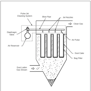
Figure 1 illustrates the pulse-jet cleaning system, consist-ing primarily of an air reservoir, a diaphragm valve, and a blowpipe. On the blowpipe, a number of holes used as jet nozzles were drilled perpendicularly to the pipe. Each nozzle is located on the top of the filter bag coaxially.

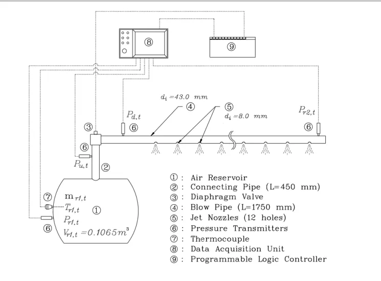
Figure 2 schematically depicts the physical model. The air reservoir and the blowpipe are referred to as voir 1 and reservoir 2, respectively. The volume of reser-voir 1 is V_r1, and the temperature, pressure, and mass of the air in reservoir 1 are T_r1,t ,P_r1,t, and m_r1,t ,respectively.

The volume of reservoir 2 is V_r2 , and the temperature, pressure, and mass of the air in reservoir 2 are T_r2,t ,P_r2,t,

Pulse-Jet

Cleaning System _{Blow Pipe}

Jet Nozzles Clean Gas Air Pulse Dust Cake Diaphragm Valve Air Reservoir Dust Laden Gas Stream Bag Filter

Figure 1. An illustration of a pulse-jet cleaning system.

and m_r2,t, respectively. Next, the subscripts u and d denote the properties of the air upstream and downstream of the diaphragm valve, respectively. The areas of the exits of res-ervoir 1 and resres-ervoir 2 are equal to the cross-sectional area of the connecting pipe A_b and the total cross-sectional area of the nozzles on the blowpipe A_n, respectively. Finally, the mass flow rates discharged from reservoir 1 and reservoir 2

are

m

&

_1,t and

m

&

2,t, respectively.

The air discharging from reservoir 1 via reservoir 2 into the atmosphere takes a relatively short time. The process is regarded as adiabatic. In addition, the volume of the con-necting pipe is much smaller than those of the reservoirs. The air properties along the connecting pipe are assumed to be the same as the diameters at the exit of reservoir 1. To facilitate the analysis, both the exits of reservoir 1 and res-ervoir 2 and the entrance of resres-ervoir 2 are assumed to be frictionless. Consequently, the processes can be expressed reasonably with the following governing equations.

Initially, to differentiate the ideal-gas equation of state with respect to time t for the both reservoirs:

V

dP

dt

m

R

dT

dt

RT

dm

d

r r t r t r t r t r 1 1 1 1 1 , , , ,

=

+

(1a) V dP dt m R dT dt RT dm dt r2 r t2, = r t2, r t2, + r t2, r2 (1b) where dm dt r t1, and dm dt r t2,

denote the mass change rates of the air in reservoirs 1 and 2 at time t, respectively. Therefore

dm

dt

m

r t t 1 1 , ,

&

= −

_(2a)

dm

dt

m

m

r t t t 2 1 2 , , ,

&

&

=

−

_(2b)

Assuming that the process is adiabatic, the internal energy change rates of the air in both reservoirs can be expressed as

(

)

d m e

dt

m h

r t r t t r t 1 1 1 1 , , , ,

&

= −

_(3a)

(

)

d m

e

dt

m h

m h

r t r t t r t t r t 2 2 1 1 2 2 , , , , , ,

&

&

=

−

_(3b) where

de

r t1,

=

c dT

v r t1, _,

h

r t1,

=

c T

p r t1,_{, and} γ = c c p v , then

tem-perature change rates in both reservoirs can be derived as

dT

dt

RT

P V

m

r t r t r t r t 1 1 2 1 1 1

1

, , , ,

(

)

&

= −

γ

(4a)

dT

dt

T T

T

P V

m

P

r t r t r t r t r t r t 2 1 2 2 2 2 2 1

1

, , , , , ,

&

(

=

γ

−

+

−

(4b)

Figure 2. Physical model.

Substituting eq 4 into eq 1, the pressure change rates of the air in the reservoirs are expressed as

dP

dt

RT

V

m

r t r t r t 1 1 1 1 , , ,

&

= −

γ

(5a)

dP

dt

RT

V

m

RT

V

m

r t r t r t r t r t 2 1 2 1 2 2 2 , , , , ,

&

&

=

γ

−

γ

_(5b)

Notably, as shown in eqs 4 and 5, the pressure and temperature change rates of the air in both reservoirs are expressed in terms of

m

&

_{1 and ,t}

m

&

_{2 .,t}

According to Saad,7 _{the mass flow rates}

&

,

m

_{1 both up-t} stream and downstream of the diaphragm valve may be expressed as ( &, , , , , m P T RA M M t u t u t b u t u t 1 0 0 2 2 1 1 2 = + −    γ γ γ (6a)

&

, , , , ,

m

P

T

R

A

M

M

t d t d t b d t d t 1 0 0 2

1

1

2

=

+ −





γ

γ

_(6b)

where the subscript 0 denotes the stagnation properties of the air. While assuming that the process is adiabatic and that the exit of reservoir 1 and the entrance of reservoir 2 are frictionless, both the stagnation tempera-tures of T_u0,t and T_d0,t are equal to T_r1,t and the stagnation pressures of P_u0,t and P_d0,t are equal to P_r1,t and P_r2,t,

respec-tively. The static properties of P_u,t, P_d,t, T_u,t, and T_d,t can be obtained from the following equations:7

P

u t,

=

P

u t,

+ −

M

u t,









− 0 2 1

1

1

2

γ

γγ (7a)

P

_{d t,}

=

P

_{d ,t}



+ −

M

_{d t,}







− 0 2 1

1

1

2

γ

γγ (7b) and

T

T

M

u t u t u t , , ,

=

+ −

0 2

1

1

2

γ

(8a)

T

T

M

d t d t d t , , ,

=

+ −

0 2

1

1

2

γ

(8b)

Based on the results of our previous study,6 _{the valve}

flow characteristics of the diaphragm valve can be ex-pressed as

( )

2

1

ln

x

C

C

G

_t

=

_t

+

₍₉₎

where C₁ and C₂ are empirical constants and the pressure ratio x_t and the dimensionless mass flow rate G_t are defined as

x

P

P

P

t u t d t u t

=

,

−

, , (10)

G

m

RT

A P

t t u t b u t

=

&

, , , 1 ₍₁₁₎

Solving eqs 6–11, the variables M_u,t , M_d,t , P_u,t, P_d,t, T_u,t,

T_d,t , x_t, G_t, and

m

&

_{1 are determined as the properties of,t}

P_r1,t ,P_r2,t ,T_r1,t, and T_r2,t.

The mass flow rate

m

&

_{2 discharged from reservoir 2,t} can be expressed as7

&

, , , , ,

m

P

T

R

A

M

M

t r t r t n n t n t 2 2 2 2

1

1

2

=

+ −









γ

γ

(12)

where M_n,t denotes the Mach number of the air flow at the exit of the nozzle and can be solved by the following equation:

P

P

M

r t atm n t 2 2 1

1

1

2

, ,

= + −



_

γ



_

− γ γ (13)

Solving eqs 12 and 13, the variables M_n,t and

m

&

2_,tare de-termined as the properties of P_r2,t , P_atm, and T_r2,t.

Therefore, both the mass flow rates of

m

&

_1,tand

m

&

2_,t are determined and are used to calculate the change rates of dT_dtr t1, , dT dt r2 ,t_, dP dt r t1, _{, and} dP dt

r2 ,t _{from eqs 4 and 5. Then the}

properties of air in the both reservoirs at next time interval can be calculated by using the forward finite difference.

The calculation procedures for solving the above equations are summarized as follows:

(1) Obtain the initial air properties of Pr_1,t, P_r2,t, T_r1,t, and T_r2,t.

(2) Assume an initial mass flow rate

m

&

,t n

1 1

=

, where the superscript n denotes the times of iteration. (3) Let P_u0,t = P_r1,t and T_u0,t = T_r1,t , then substitute Pu0,t,

Tu0,t, and

m

&

₁n_,tinto eq 6a and calculate the up-stream Mach number M_{u t}n_, .

(4) Substitute P_u0,t and

M

u t n

, into eq 7a and calculate

the upstream static pressure

P

_{u t}n_, . (5) Substitute T_u0,t and M_{u t}n

, into eq 8a and calculate

the upstream static temperature

T

u t n ,.

(6) Substitute

P

_{u t}n_, ,

T

_{u t}n

, , and

m

&

,t n

1 into eq 11 and

cal-culate the dimensionless mass flow rate

G

t n

. (7) Substitute

G

_tn into eq 9 and calculate the

pres-sure ratio

x

t n . (8) Substitute

P

u t n , and

x

t n

into eq 10 and calculate the downstream static pressure

P

_{d t}n

, .

(9) Substitute

m

&

,t n

1 and

P

d t n

, into eqs 6b and 7b,

re-spectively, and calculate the downstream stag-nation pressure

P

d tn0, and Mach number

M

d t

n

, .

(10) Adjust

m

&

₁n_,t to

m

&

₁n_,t+1 and iterate from step 3 to step 9 until the conditions of M_{d t}n n

, = +1_{− <1 10}−6 _and P_dn_t P r t 0, ≥ 2, or the conditions of

(

P P

)

P d t n r t r t 0 1 2 2 6 10 , , , + − − < and Md t n , ≤1are satisfied.

(11) Substitute P_r2,t and P_atm into eq 13 and calculate the Mach number Mn,t.

(12) Substitute P_r2,t, T_r2,t, and Mn,t into eq 12 and ob-tain the mass flow rate

m

&

_2,t.

(13) Substitute Tr_1,t, T_r2,t, Pr_1,t, P_r2,t,

m

&

₁n_,t, and

m

&

_2,tinto eqs 4 and 5 and obtain the temperature and pres-sure change rates of dT

dt r t1, _, dT dt r2 ,t_, dP dt r t1, , and dP dt r2 ,t

for both reservoirs.

(14) Use the forward finite difference to obtain the properties of the air in the reservoirs at next time step

t

+ ∆

t

.

T

T

dT

dt

t

r t t r t r t 1 1 1 , , , +∆

=

+

∆

(14a)

T

T

dT

dt

t

r t t r t r t 2 2 2 , , , +∆

=

+

∆

(14b)

P

P

dP

dt

t

r t t r t r t 1 1 1 , , , +∆

=

+

∆

(14c)

P

P

dP

dt

t

r t t r t r t 2 2 2 , , , +∆

=

+

∆

(14d) (15) Replace P_r1,t , P_r2,t , T_r1,t and T_r2,t byPr t1,+∆t , Pr t2,+∆t ,

Tr t1,+∆t _and Tr t2,+∆t , respectively, in step 1; (16) Iterate from step 2 to step 15 until the time of

the diaphragm valve is closed. Meanwhile, the values of

m

&

_1,t , dP

dt

r t1, _and dT

dt

r t1, _{are zero; and}

(17) Iterate from step 11 to step 15 until the pressure of

P_r2,t is equal to the atmospheric pressure P_atm.

EXPERIMENTAL APPARATUS AND PROCEDURE

Experiments were performed to examine the feasibility of the proposed model. Figure 3 illustrates the experimen-tal apparatus. An air reservoir (1) with a volume of 0.1065 m3 _{was used. The pressure P}

r1,t and temperature Tr1,t of the air in the air reservoir were measured by the pressure trans-mitter (6) and the thermocouple (7), respectively. A con-necting pipe (2) with a diameter of 43 mm and a length of 450 mm was used to connect the air reservoir and the diaphragm valve (3). The diaphragm valve had a nomi-nal diameter of 1.5 in. Two pressure transmitters (6) were installed separately on both sides of the diaphragm valve to measure the pressure variations of P_u,t and P_d,t during the discharge process. Next, a blowpipe (4) with a length of 1750 mm and a diameter of 43 mm was connected at the downstream of the diaphragm valve. On the blow-pipe, twelve nozzles (5) with a diameter of 8 mm were drilled perpendicularly to the blowpipe. Another pressure transmitter was installed at the end of the blowpipe to measure the stagnation pressure P_r2,t of the air in the blow-pipe. Finally, a programmable logic controller (PLC) (9) was used to generate the trigger for opening the diaphragm valve and starting the data acquisition unit (8).

Procedures of the experimental work were as follows: (1) Measure and record the initial state pressure

P_r1,t=i and temperature T_r1,t=i of the air in the air reservoir under a stable situation.

(2) Execute the PLC program to open the diaphragm valve under a designed duration t and start the data acquisition unit.

(3) Measure and record the pressure variations of P_r1,t,

P_u,t, P_d,t, and P_r2,t.

(4) Measure and record the final state pressure P_r1,t=f and temperature T_r1,t=f of the air in the reservoir under a stable situation. The final state implies that the experimental work is completed and the values of P_r1,t and T_r1,t of the air in the reservoir are invariant.

(5) Change the test condition and repeat the above procedures until enough data are obtained. Prior to conducting the experimental work, the sure transmitters used were calibrated by a standard pres-sure gauge. These prespres-sure transmitters are made of the TRANSBAR ceramic sensing element. The measuring range is 0–10 bar. The error is within 0.2% of full scale. The typical response time is less than 3 msec. These pressure transmitters are calibrated by a WIKA standard pres-sure gauge, which has a measuring range of 0–10 kg/ cm2_{, a scale division of 0.05 kg/cm}2_{, and accuracy}

within 0.5% of full scale. Calibration results indicated that the discrepancies between the readings of the stan-dard pressure gauge and those of the pressure trans-mitters were within 0.5%.

RESULTS AND DISCUSSION

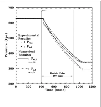
Figure 4 presents the pressure variations during the dis-charge process. Figure 4a illustrates the pressure variations of P_r1,t and P_u,t. Figure 4b illustrates the pressure variations of P_d,t and P_r2,t. In this case, the duration of the electric pulse was 500 msec (from t = 400 msec to t = 900 msec). Due to the mechanical delay of the diaphragm valve, the beginning and the end of the variations of the pres-sures measured were slower than those of the electric pulse signals. These delays are estimated to be 30 msec and 150 msec, respectively.

After the diaphragm valve was opened, air was charged from the air reservoir into the blowpipe. The dis-charged air decreased the pressures of P_r1,t and P_u,t and in-creases the pressures of P_d,t and P_r2,t. After the pressure of

P_r2,t increased to a maximum value, all of the pressures of

P_r1,t , P_u,t, P_d,t, and P_r2,t monotonously decreased with time. At the moment the diaphragm valve was completely closed, the pressures of P_r1,t and P_u,t reached their minimums. Af-ter that, the pressures of P_r1,t and P_u,t gradually reached thermodynamic equilibrium. Meanwhile, the mass in the air reservoir m_r1,t remained unchanged. The pressures of P_d,t and P_r2,t continuously decreased, however, until both pres-sures equaled the atmospheric pressure P_atm.

In the numerical calculations, the empirical constants

C₁ and C₂ used in eq 9 are obtained from the results of our earlier study6 _{and were equal to 0.1012 and 0.3933,}

respectively. The beginning of the discharge process was t

= 430 msec, which equals the electric pulse turn-on time

of t = 400 msec plus the diaphragm valve open delay time of 30 msec. The end of the discharge was t = 1050 msec, which equals the electric pulse turn-off time t = 900 msec plus the diaphragm valve close delay time 150 msec. Fig-ure 4 indicates that the decreasing rates of P_r1,t of the model prediction were greater than those of the experimental results. This phenomenon reveals that the prediction of the mass flow rate appears to be overestimated.

Figure 3. Experimental apparatus.

Directly measuring the mass flow rate of a compress-ible transient process is extremely difficult. Therefore, to directly validate the accuracy of the mass flow rates pre-dicted by the proposed model is impossible. According to our earlier study,6 _{however, the residual mass m}

r1,t in the air reservoir and the mass flow rate

m

&

_1,t discharged from the air reservoir of an adiabatic process can be calculated from the pressure variation of P_r1,t as

m

m

P

P

r t r t i r t r t i 1 1 1 1 1 , , , ,

=













= = γ (15)

&

, , , , , ,

m

dm

dt

m

P

P

P

t r t r t i r t r t r t 1 1 1 1 1 1

1

= −

= −







= =

γ

(16)

Figure 5 illustrates the results of m_r1,t calculated from eq 15 by substituting the measured P_r1,t shown in Figure 4 into the equation. In addition, Figure 5 also illustrates the residual mass (m_r1,t )_iso of an isothermal process to com-pare with the results from eq 15. The residual mass (m_r1,t )_iso

is the lower limit of the realistic phenomena and can be calculated by the following equation:

( )

m

m

P

P

r t _iso r t i r t r t i 1 1 1 1 , , , ,

=

= = (17)

According to Figure 5, the initial mass m_r1,t=i and the final mass m_r1,t=f are obtained by substituting the initial air properties (P_r1,t=i , T_r1,t=i) and the final air properties (P_r1,t=f ,

T_r1,t=f ) into the ideal-gas equation of state. The final prop-erties refer to a situation in which the experimental work is completed and the pressure and temperature of the air in the air reservoir are unchanged and can be accurately measured. Therefore, the difference between mr_1,t=i and eq 14c

eq 7a

Figure 4(a). The pressure variations of Pr1,t and Pu,t under the

condition of 12 jet nozzles.

eq 7b

eq 14d

Figure 4(b). The pressure variations of Pd,t and Pr2,t under the

condition of 12 jet nozzles.

eq 15

eq 17

Figure 5. The variation of the residual mass of mr1,t under the condition

of 12 jet nozzles.

m_r1,t=f is 0.291 kg, which is reasonably regarded as the actual cumulated mass discharged

∆

m

_{r t i f1,=,} during the discharge process. The residual mass at the end of dis-charge of an adiabatic process and that at the end of an isothermal process—m_r1,t=e and (m_r1,t=e)_iso —are calcu-lated by substituting the pressure P_r1,t=e at the end of

discharge into eq 15 and eq 17, respectively. By doing so, the cumulated mass discharged by an adiabatic process

∆

m

r t i e1,=, and by an isothermal process

(

∆

m

_{r t i e iso1,=,}

)

were obtained and were equal to 0.278 kg and 0.359 kg, respectively. Notably, the deviation between

∆

m

_{r t i e1,=,} and

∆

m

_{r t i f1,=,} was only 4.3%, which is much smaller than that between

∆

m

_{r t i e1,=,} and

(

∆

m

_{r t i e iso1,=,}

)

, which was 23.4%. Table 1 compares the cumulated mass discharge obtained from eq 15 and from experimental work under different operating conditions. All the devia-tions are smaller than 5%. From the above discussion, we can infer that the assumption that the process is adiabatic is adequate and that the results from eq 15 are accurate.

Because eq 16 is derived from eq 15, the mass flow rate

m

&

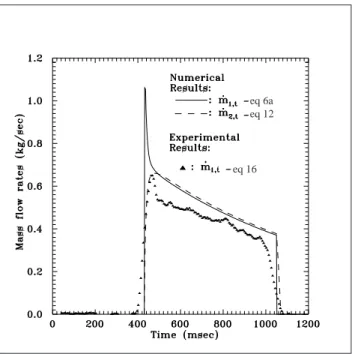
_1,tcalculated from eq 16 is regarded to be accurate and is regarded as the benchmark solution for the nu-merical result obtained from the two-reservoir model pro-posed in this study. More extensive discussions on the accuracy of the mass flow rate calculated from eq 16 can be found in our previous study.6

Figure 6 illustrates the numerical results of the mass flow rate

m

&

1,tand

m

&

2,t obtained from the proposed model and the experimental results of the mass flow rate

m

&

1,t cal-culated from eq 16. Apparently, the values of

m

&

_{1 and,t}

&

,

m

_{2 in the numerical results are close to each other andt} are greater than the value of

m

&

_{1 of the experimental re-,t} sults. This finding implies that the mass flow rates pre-dicted by the proposed model are overestimated. Except for the beginning and end of the discharge, the deviation

between the mass flow rate

m

&

1 of the experimental re-,t

sults and the numerical results from t = 500 msec to t

= 900 msec is about 10%. The deviations are more

sig-nificant at the beginning and the end of the discharge. This is because although the diaphragm valve is assumed to be immediately fully opened or closed in model calcula-tion, it is gradually opened or closed in an actual situation. To obtain more accurate results, some modifications of the two-reservoir model are adopted. Herein, both the friction effects induced by the exit of the air reservoir and the nozzles of the blowpipe are considered. Initially, the friction effect induced by the exit of the air reservoir is represented by that of a frictional constant cross-sectional area pipe with a parameter of 4 fL

D

e h

. According to Saad,7

the relation between the Mach numbers of M_1,t and M_2,t at both sides of the frictional pipe can be expressed as

4

1

1

1

1

2

1 2 2 2

fL

D

M

M

e h t t

=



−









 + +

γ

γ

γ

, ,

ln

(18)

The average friction coefficient f is defined as

f

L

_e

fdx

Le

=

1

∫

0 (19)

Notably, the parameter of

4 fL D

e

h is obtained in advance

prior to use the proposed model. Various methods are avail-able to determine the value of 4 fL

D e h

. Herein, a relatively simple method is proposed as an alternative to determine the parameter of 4 fL_De

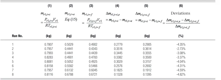
h . The method is described as follows. Table 1. The comparisons of the cumulated mass discharged between the experimental results and those obtained from eq 15.

(1) (2) (3) (4) (5) (6) Run No. (kg) (kg) (kg) (kg) (kg) (%) 1 0.7807 0.5029 0.4902 0.2779 0.2905 -4.35% 2 0.7957 0.4441 0.4343 0.3516 0.3614 -2.73% 3 0.7993 0.4441 0.4439 0.3445 0.3555 -3.08% 4 0.8283 0.4901 0.4783 0.3382 0.3500 -3.37% 5 0.8081 0.5052 0.4925 0.3029 0.3157 -4.04% 6 0.8158 0.5582 0.5466 0.2576 0.2692 -4.31% 7 0.7957 0.6132 0.6045 0.1825 0.1912 -4.59% 8 0.8116 0.6788 0.6721 0.1328 0.1395 -4.82% Deviations

Displacing the stagnation pressure P_u0,t in eq 6a by

P_r1,t and substituting the mass flow rate

m

&

1_,t obtained from eq 16 into eq 6a allows us to calculate the Mach number

M_1,t . On the other hand, the mass flow rate

m

&

1_,t can be expressed in terms of the static pressure of P_u,t as7

&

, , , ,

m

P

T

R

A M

M

t u t r t b u t u 1 1

1

1

2

=

γ

+ −

γ

(20) Substituting the measured static pressure P_u,t measured and the mass flow rate

m

&

1_,t obtained from eq 16 into eq 20 allows us to obtain the Mach number M_u,t , which is

regarded as M_2,t in eq 18. Finally, substituting the

deter-mined Mach numbers M_1,t and M_2,t into eq 18 allows us to calculate the parameter of 4 fL_De

h .

Figure 7 illustrates the Mach numbers M_1,t and M_2,t and the parameter 4 fL_De

h . Except for the beginning and end

of the discharge, the time average value of 4 fL

D e h

from t =

500 msec to t = 900 msec is about 0.74.

As for the nozzles on the blowpipe, the friction effect resulted in a mass flow rate discharged from an actual nozzle that was lower than that discharged from an ideal nozzle. Therefore the real mass flow rate

m

&

_2,t discharged from the blowpipe can be expressed by introducing the discharge coefficient Cd_n into eq 12 as

&

, , ,

m

P

T

R

A C

M

M

t r t r t n dn n 2 2 2

1

1

2

=

+ −





γ

γ

(21) In the model calculations, the value of Cd_n must also be known in advance. The value of Cd_n is usually

determined according to the standard test procedure of ANSI/ASME8_{. Herein, an alternative is proposed to}

deter-mine the value of Cd_n by using the measured pressure variations shown in Figure 4. In addition to the fact that the volume of the blowpipe is markedly smaller than that of the air reservoir, the discharge process is extremely rapid and the value of

m

&

1,tis close to the value of

&

,

m

2tat the same time t. Therefore the value of T_r2,t is considered to be equal to the value of Tr_1,t. In addi-tion, the time-dependent temperature T_r1,t can be cal-culated by the following equation:

T

T

P

P

r t r t i r t r t i 1 1 1 1 1 , , , ,

=













= = − γ γ (22)

Therefore the mass flow rate

( )

m&2,_{t isen}of an insentropic

flow can be determined by substituting the stagnation temperature T_r2,t (_{= Tr1,t} ) and the measured pressure P_r2,t into eq 12. Then the discharge coefficient Cd_n can be deter-mined by the following equation:

( )

( )

, 1 , 2 , 2 , 2

1





 +

≈

=

γ

γ

t r t r isen t real t n

R

T

P

m

m

m

Cd

&

&

&

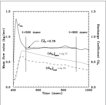
(23) Where the Mach number M_n,t is calculated by substi-tuting the measured pressure P_r2,t into eq 13.

Figure 8 plots the results of

( )

m&2,t _realfrom eq 16,

( )

m&2,t _isenfrom eq 12, and C_dn obtained from eq 23. eq 6a

eq 12

eq 16

Figure 6. The variations of the mass flow rate of

m

&

1,tand

m

&

2,t

under the condition of 12 jet nozzles.

eq 18

eq 18

Figure 7. The variations of the Mach number of Mu,t and the parameter

of 4 fL D

e h

under the condition of 12 jet nozzles.

Cd_n

Except for the beginning and end of the discharge, the average value of Cd_n from t = 500 msec to t = 900 msec is about 0.78.

As the parameters of 4 fL D

e h

and Cd_n are adopted into the model, some of the calculation procedures must be modified as follows.

(a) Divide step 3 in the above calculation procedure into three parts: 3-1, 3-2, and 3-3.

(3-1) Displace P_u0,t and T_u0,t by P_r1,t and T_r1,t in eq 6a, respectively. And then the Mach num-ber

M

u t

n

, is calculated and regarded

as

M

t n

1, in eq 18.

(3-2) Substitute the values of 4 fL_De

h (= 0.74)

and

M

t n

1, into eq 18 to obtain the Mach

number

M

_2,n_t.

(3-3) Displace

M

_{u t}n_, by

M

t n

2, in eq 6a and

ob-tain the value of

P

u t n

0, .

(b) Renew step 4. Substitute

P

u t n

0, and

M

u t

n

, into eq

7a and calculate the upstream static pressure

P

u t n

, .

(c) Renew step 12. Substitute P_r2,t, T_r2,t, and Mn,t into eq 21. In doing so, the mass flow rate of m&2,t is

obtained.

Figure 9 illustrates the variations of pressures and the mass flow rates of the model predictions and the experi-mental results. In model calculation, the values of 4 fL_De

h

and Cd_n are equal to 0.74 and 0.781, respectively. Experi-mental results are the same as those shown in Figures 4 and 6. Figure 9 indicates that all of the pressures and mass flow rates of the model predictions agree well with the experimental results. The deviation between the average mass flow rate of

m

&

_{r t1,}from t = 500 msec to t = 900 msec of the model predictions and the bench mark solutions is about 0.61%.

For validating the proposed model, some of the nozzles on the blowpipe are blocked to change the total discharge area A_n of the blowpipe. Figure 10 summa-rizes the results of the variations of the pressures and of the mass flow rates, which are obtained under the condition of eight nozzles being opened and four nozzles being blocked. The values of Cd_n and 4 fL

D

e h

em-ployed in the model are the same as those used in the previous case. According to Figure 10, the variations of the pressures and the mass flow rates of the numeri-cal results well with the experimental results. The de-viation between the average mass flow rate of

&

,

m

r t1 from t = 500 msec to t = 900 msec of the model

predictions and the bench mark solutions is about 0.85%. Table 2 compares the average mass flow rates under different discharge areas. The maximum devia-tion between the numerical and experimental results is smaller than 3%. Obviously, considering the fric-tion effects of the exits of both reservoirs significantly improves the accuracy of the model predictions.

CONCLUSION

This study presents a novel two-reservoir model to simu-late the air discharged from an air reservoir via a dia-phragm valve to a blowpipe and ultimately into the at-mosphere of a pulse-jet cleaning system. Based on the results in this study, we can conclude the following:

(1) Without considering the friction effects of the exits of both reservoirs, the mass flow rates of the model predictions are about 10% overestimated. (2) Introducing a parameter of 4fLe/D_h and a

dis-charge coefficient Cd_n into the governing equa-tions allowed us to successfully simulate the fric-tion effects induced by the exit of the air reser-voir and the nozzles on the blowpipe. The ex-perimental methods to determine both 4fLe/D_h and Cd_n are also presented.

(3) The proposed model is more accurately simulated by considering the friction effects induced by the exit of the air reservoir and the nozzles on the blowpipe. The accuracy is significantly improved. Deviations between the mass flow rates of the model predictions with those of the bench mark solutions are smaller than 3%. Moreover, the pres-sure variations of the model predictions agree well with those obtained by experimental work.

ACKNOWLEDGMENT

The authors would like to thank the National Science Council of the Republic of China and the Taiwan Power Company for financially supporting this research under Contract No. NSC-87-TPE-E-009-007.

eq 12

eq 16

Figure 8. The variations of the mass flow rate of m&1,tand m&2,t and

the discharge coefficient Cdn under the condition of 12 jet nozzles.

eq 14c eq 7a eq 14d eq 7b eq 16 eq 6a eq 12

Figure 9. (a)The pressure variations of Pr1,t and Pu,t under the condition

of 12 nozzles. (b). The pressure variations of Pd,t and Pr2,t under the

condition of 12 nozzles. (c). The variations of the mass flow rate of

&

,

m

_1tand

m

&

2,t under the condition of 12 nozzles.

Figure 10. (a) The pressure variations of Pr1,t and Pu,t under the

condition of 8 nozzles. (b) The pressure variations of P_d,t and P_r2,t under the condition of 8 nozzles. (c) The variations of the mass flow rate of

&

,

m

_1tand

m

&

_2,t under the condition of 8 nozzles.

eq 14c eq 7a eq 14d eq 7b eq 6a eq 16 eq 12 (a) (b) (c) (a) (b) (c)

NOMENCLATURE

Ab = blowpipe cross-sectional area, m2

An = total cross-sectional area of the nozzles on the blowpipe, m2

Cp = constant-pressure specific heat, kJ/(kg K)

Cv = constant-volume specific heat, kJ/(kg K)

C₁, C₂ = constant

Cd_n = discharge coefficient of the nozzle, ratio of the real mass flow rate to the mass flow rate of an isentropic flow, =

( )

( )

& & m m real isen , dimensionless d = diameter, m D_h = hydraulic diameter, m

e = specific internal energy of air in a reservoir, kJ/kg

f = friction factor, dimensionless

G = dimensionless mass flow rate, defined by eq 11, dimensionless

h = specific enthalpy of air in a reservior, kJ/kg

m = mass of air in a reservior, (= PV/RT), kg

∆m = cumulated mass discharged, kg

&m

= mass flow rate discharged from flow reservoir, kg/sec

M = Mach number, dimensionless Patm = atmospheric pressure, kPa

P = absolute pressure, kPa

R = gas constant of air, (=287.04), m2_/(s2 _K) T = temperature, K

V = volume, m3

x = ratio of pressure drop to absolute upstream

pres-sure, (=(P_u-P_d )/P_u), dimensionless

= ratio of specific heats, (=Cp/Cv), dimensionless Subscripts

0 = stagnation properties

r1 = the reservoir 1, (the air reservoir)

r2 = the reservoir 2, (the blowpipe)

u = the upstream of the diaphragm valve

d = the downstream of the diaphragm valve

i = the initial state

e = at the end of discharge

f = the final state

t = time Superscript

n = times of iteration

REFERENCES

1. Morris, W.J. “Cleaning mechanisms in pulse jet fabric filters,”

Filtra-tion & SeparaFiltra-tion 1984, 21, 50-54.

2. Bouilliez, L. “Importance of physical parameters for the cleaning

effi-ciency of a reverse jet-cleaned dust collector,” Solids Handling Con-ference, Harrogater, England, 1986, pp B11-B25.

3. Sievert, J.; Löffler, F. “The effect of cleaning system parameters on the pressure pulse in a pulse-jet filter,” Particulate and Multiphase Processes

Conference, Miami, FL, 1987; Vol.2, pp 647-662.

4. De Ravin, M.; Humphries; W.; and Postle, R. “A model for the

perfor-mance of a pulse jet filter,” Filtration & Separation 1988, 25, 201-207.

5. Hajek, S.; Peukert, W. “Experimental investigations with ceramic

high-temperature filter media,” Filtration & Separation 1996, 33, 29-37.

6. Fu, W.S.; Ger, J.S. “A concise method for determining a valve flow

coefficient of a valve under compressible gas flow,” Experimental

Ther-mal & Fluid Sci., in press.

7. Saad, M.A. Compressible Fluid Flow; 2nd ed.; Prentice Hall: New Jersey,

1993; Chapter 3.

8. Performance Test Cords on Safety and Relief Valves; The American

Soci-ety of Mechanical Engineers: New York, 1976; ANSI/ASME PTC 25.3-19.

Table 2. The comparisons of the average mass flow rates between the experimantal results and the numerical results.

Experimental Conditions Average Mass Flow Rate from t=500 msec to t=900 msec

Initial Initial Jet Nozzles Experimental Results Numerical Results Deviations Remark

Pressure Temperature Opened/Blocked eq 16 4fL_e/D_h=0.74

P_r1,t=I T_r1,t=I Cd_n=0.78

(kpa) (K) (kg/sec) (kg/sec) (%)

629.7 293.7 12 / 0 0.4602 .04574 -0.67% Fig. 9c 515.8 298.8 12 / 0 0.3755 0.3744 -0.29% 514.5 299.1 8 / 4 0.2859 0.2835 -0.85% Fig. 10c 512.8 299.0 4 / 8 0.1624 0.1596 -1.74% 517.1 299.1 2 / 10 0.0894 0.0867 -2.99% 517.9 299.4 1 / 11 0.0469 0.0458 -2.31%

About the Authors

Dr. W.S. Fu is a professor in the Mechanical Engineering Department of Chiao Tung University, Hsinchu, 30050, Tai-wan, R.O.C. J. S. Ger is a Ph.D. student in the Mechanical Engineering Department of Chiao Tung University and a re-searcher in the Energy & Resources Laboratories of Indus-trial Technology Research Institute. Correspondence should be sent to Dr. W.S. Fu, Professor, Mechanical Engineering Department, Chiao Tung University, 1001 Ta Hsueh Rd., Hsinchu, 30050, Taiwan, R.O.C.