多重社群的相似指數研究

行政院國家科學委員會專題研究計畫 成果報告

多重社群的相似指數研究

研究成果報告(精簡版)

計 畫 類 別 ： 個別型 計 畫 編 號 ： NSC 96-2118-M-004-003- 執 行 期 間 ： 96 年 08 月 01 日至 97 年 07 月 31 日 執 行 單 位 ： 國立政治大學統計學系 計 畫 主 持 人 ： 余清祥 計畫參與人員： 此計畫無其他參與人員： 報 告 附 件 ： 出席國際會議研究心得報告及發表論文 處 理 方 式 ： 本計畫涉及專利或其他智慧財產權，1 年後可公開查詢

中 華 民 國 97 年 09 月 09 日

1

行政院國家科學委員會補助專題研究計畫成果報告

多重社群的相似指數研究

A Similarity Index Among Multiple Populations

計畫編號： NSC 96-2118-M-004 -003

執行期限：96 年 8 月 1 日至 97 年 7 月 31 日

主持人：余清祥 執行單位：國立政治大學統計系

一、中文摘要 物種相似性為兩個族群中有物種的相 似程度測量值，可用於比較兩個地區生態環 境的相似程度，或是評估某族群在不同時間 的變遷。過去，生態學家曾使用物種重複評 估諸如珊瑚、水鳥等生物族群間的相似性及 其變遷；近年來也應用於網際網路搜尋引 擎，查詢比對資料的相似性。較為常用的相 似指數為 Jaccard 指數，其定義為相同品種 個數的比例，並未將品種在族群中佔有的比 例及可能遷移的特性列入考慮，無法反映各 品種間的生態競爭問題，參考 Yue 等人 (2001, 2005)的討論。 本研究以探討多重社群的相似指數為 目的，首先研究回顧現有的兩兩社群間的相 似指數，並將其延伸至多重社群。本文除了 探討如何將變異數分析延伸至多重社群的 相似指數，並以最大概似估計求取相似指數 的估計量，以理論及電腦模擬研究估計量的 在大樣本及小樣本的特性。 關鍵詞：相似指數、生物多樣性、Jaccard 指數、 Simpson 指數、Shannon 指數、最大概似估計 Abstract

Most species diversity indices are designed to measure the species diversity of one population or two populations. For example, the Shannon and Simpson indices are for one population and the Jaccard index is for two populations. There are only a few for the similarity among three or more populations. In

this study, we propose a class of similarity indices for multiple populations, to measure the ratio of between-population characteristics and within-population characteristics.

The focus of the study is to review the similarity indices and propose a similarity index for measuring 3 or more populations. The proposed index will adapt the idea of Analysis of Variance in measuring treatment effect. We will use the Maximum likelihood estimation to find the estimator and study its asymptotic properties.

Keywords: Similarity index; Species diversity; Jaccard Index; Simpson index; Shannon Index; Maximum likelihood estimator

二、緣由與目的

Similarity index originally was studied in ecology, biology, and biogeography, to measure the species diversity between two populations, or the change of a population over time. It receives more attentions and applications in recent years due to the growing needs of analyzing large data sets. Search engine on the web is a famous application of using the similarity index. Most search engines require users typing keywords and a similarity index value of each web page is calculated based on these keywords. Then the closeness of web page with respect to the keywords is sorted according to the similarity values.

To compute the similarity index for each population and then judge the closeness of any two populations is one way to decide if two populations are similar. This is more efficient

and more convenient for the web search. Another way to decide if two populations are similar is to compute the similarity indices of two populations. Similarity indices for two populations include the Jaccard index, Morisita index, Smith’s index (Smith et al., 1996), and Yue’s index (Yue and Clayton, 2005). Although the between-population similarity indices are likely to be underestimated, they are preferred to the similarity indices of each population.

Although the demands of measuring similarity among three populations and more are growing, most studies still focus on measuring the similarity of one or two populations and only a few discuss the extension to more than two populations. Lande (1996) perhaps is the only work talking about the extension of measuring the similarity of two populations to that of three populations and more. He used the notion analogical to the analysis of variance (ANOVA) and separate total species diversity into between and within species diversity. The species diversity considered needs to satisfy the concavity property in order to be extended to measure the similarity of three populations.

三、多重母體相似指數

In this section, we shall use the Simpson index to demonstrate the proposed similarity index. The Simpson index is the probability of obtaining same species if two observations are sampled. The Morisita index and Yue’s index (Yue and Clayton, 2005) can be treated as the two-population Simpson index. For example, the Morisita index is defined as

∑

∑

∑

= = = + = _S i i S i i S i i i M q p q p 1 2 1 2 1 2

θ , where S is the number of

species in two populations,0≤ p_i,q_i ≤1, and are the proportions of the ith species in populations 1 and 2, respectively. The numerator (i.e., between effect) of the Morisita index is the probability of obtaining same

species if one observation is taken from each population. The denominator (i.e., within effect) of the Morisita index is the probability of obtaining same species if two observations are taken from one of two populations. If these two populations are similar with respect to species proportions, i i q p & M θ will be close to 1, since sampling from two identical populations is equivalent to sampling from any one of the populations.

Therefore, the Morisita index is the ratio of the between Simpson index to the within Simpson index. To further extend the Lande’s notion of similarity index being the ratio of between and within characteristics, we define a generalized Simpson index for three populations and more as ⎟⎟ ⎠ ⎞ ⎜⎜ ⎝ ⎛ ⎥ ⎦ ⎤ ⎢ ⎣ ⎡ ⎟⎟ ⎠ ⎞ ⎜⎜ ⎝ ⎛ ⎥ ⎦ ⎤ ⎢ ⎣ ⎡ =

∑ ∑

∑ ∑

≤ ≤ ≤ < ≤ 1 2 1 2 1 * m p m p p m j i ij m k j i ik ij S θ (1)

where p_ij is the species proportion of species i

for population j, for j = 1, 2, …, m,

and S is the total number of species in Populations 1 to m. It is obvious that the Morisita index is a special case of (1) with m =

2. Also, can be shown by the fact

that .

∑

= = S i ij p 1 1 1 0≤θ_S* ≤ ik ij ik ij p p p p2+ 2 ≥2

Note that this index is the ratio between two Simpson indices. The index on the numerator is the probability that, randomly selecting two populations and randomly sampling an observation from each population, these two observations are of the same species. The denominator is the probability that, randomly selecting one population and randomly sampling two observations from this population, these two observations are of the same species. In other words, the numerator is the “average” between Simpson index and the denominator is the “average” within Simpson index.

四、最大概似估計

The maximum likelihood estimator can be

used for the similarity index in (1), similar to

that in Yue and Clayton. Let and

. Thus, the similarity index in (1)

is equivalent to

∑

= = S i ij j p a 1 2

∑

= = S i ik ij jk p p d 1 A m D a m d S j j m k j jk S ) 1 ( 2 ) 1 ( 2 1 1 * − = − =

∑

∑

= ≤ < ≤ θ . Suppose that

∑

= ⎟ ⎟ ⎠ ⎞ ⎜ ⎜ ⎝ ⎛ = S i j ij j n X a 1 2 ˆ and

∑

= ⎟⎟⎠ ⎞ ⎜⎜ ⎝ ⎛ ⎟ ⎟ ⎠ ⎞ ⎜ ⎜ ⎝ ⎛ = S i k ik j ij jk n X n X d 1 ˆ _{, where is the}

number of occurrences for the ith species from observations taken from the jth population.

ij

X

j

n

Then, we can use

A m D a m d m j j m k j jk S _ˆ ) 1 ( ˆ 2 ˆ ) 1 ( ˆ 2 ˆ 1 1 * − = − =

∑

∑

= ≤ < ≤ θ as the estimate of θˆS* (NPMLE). As Min{n1,n2,K,nm}→∞,

we can show that and in

probability, which implies that in

probability according to Slutsky’s lemma.

j j a aˆ → dˆ_jk →d_jk * * ˆ S S θ θ →

The asymptotic variance of can be

derived via Cramer’s delta method and approximately * ˆ S θ ⎥ ⎦ ⎤ ⎢ ⎣ ⎡ − + ⎟ ⎠ ⎞ ⎜ ⎝ ⎛ − = (ˆ,ˆ) ˆ ˆ 2 ) ˆ ( ˆ 1 ) ˆ ( ˆ ˆ 1 2 ) ˆ ( _{4 2 3} 2 2 * D A Cov A D D Var A A Var A D m VarθS (2) where

∑ ∑

= = ⎟ ⎠ ⎞ ⎜ ⎝ ⎛ − ≅ m j S i j ij j a p n A Var 1 1 2 3 4 ) ˆ ( ,

∑

∑

∑

≤ < ≤ = = ⎟ ⎟ ⎠ ⎞ ⎜ ⎜ ⎝ ⎛ + − + ≅ m k j jk k j S i ik ij k S i ik ij j d n n p p n p p n D Var 1 1 2 1 2 ) 1 1 ( 1 1 ) ˆ (

∑∑ ∑

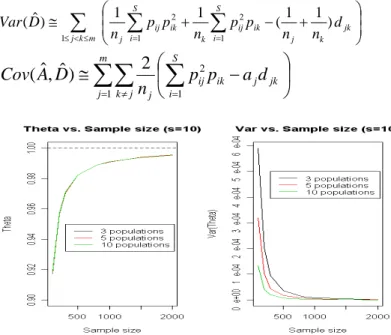
= ≠ = ⎟ ⎠ ⎞ ⎜ ⎝ ⎛ ₋ ≅ m j k j S i jk j ik ij j d a p p n D A Cov 1 1 2 2 ) ˆ , ˆ (

Figure 1. Similarity index vs. number of populations (uniform dist.)

Example 1. Suppose there are some identical populations, with the number of species being 10, and the species proportions follow uniform distribution. Figure 1 shows the results of similarity index values vs. the number of populations (1,000 simulation runs). We can see that the mean value of the index is not influenced by the number of populations. However, as noted in Chao et al. (2006), the similarity index based on the number of occurrences (like the proposed θ) is usually under-biased in uniform distribution. Also, the variance of the index depends on the sample size and the number of populations. We can also see that the variance is also a function of the number of populations and decreases faster than the speed of sample size.

To further investigate the relationship of sample size and variance, we plot the graphs of sample size vs. n×variance and sample size vs. n×s.e. (Figure 2). It is interesting to see that the variance of looks like a constant, no matter what the number of populations is. The reason for much faster convergence could be that

in for a uniform

distribution. We shall check the case of other distributions. θˆ 0 1 2 3− ≅

∑

= S i j ij a p Var(Aˆ) 3

七、參考文獻

z Emigh, T. H. (1983). On the Number of Observed Classes from a Multinomial Distribution. Biometrics 39:485-491. z Chao, A., Chazdon, R. L., Colwell, R. K.,

and Shen, T. (2006). Abundance-Based Similarity Indices and Their Estimation when There are Unseen Species in Samples. Biometrics 62:361-371.

Figure 2. Variance of Similarity index vs. number of populations (uniform dist.)

z Feller, W. (1968). An Introduction to Probability Theory and its Applications, vol. 1, 3PrdP ed. New York: Wiley.

六、結論與建議

In this study, we propose a probabilistic approach to measure multiple-community similarity. In particular, the similarity index can be computed recursively and is adapted from the set theory, which is used in Yue et al. (2001) and Yue and Clayton (2005). The proposed similarity index can be separated into measuring various order of similarity, and thus can provide more thorough information of shared species. If we are to sampling species, the proposed similarity index can be treated as a generalization of the Jaccard index and the index by Smith et al. (1996). If one observation is taken from each community, then the proposed approach can be generalized to indices similar to the Morisita index.

z Lande, R. (1996). Statistics and Partitioning of Species Diversity, and Similarity among Multiple Communities. OIKOS 76:5-13.

z Yue, J. C., Clayton, M. K., Lin, F. (2001). A Nonparametric Estimator of Species Overlap. Biometrics 57:743-749.

z Yue, J. C., Clayton, M. K. (2005). An Overlap Measure based on Species Proportions. Comm. Statist. Theory Methods 34:2123-2131.

Note that Lande (1996) also proposed a similarity index for multiple communities, but there are two main differences between our and his approaches. The similarity indices by Lande are based on the species diversity of one population and are different to our similarity indices, where ours are extension of frequently used two-population indices and our goal is to measure real similarity between 2 populations. Thus, our similarity indices have probability interpretation.

Still, there are limitations in applying the proposed similarity index. For example, the leave-one-out method can be used to verify whether there are any communities significantly different to others. Nonetheless, there are no suggestions for picking up these different communities.

出席國際學術會議心得報告

計畫編號 NSC 96-2118-M-004 -003 計畫名稱 多重社群的相似指數研究 出國人員姓名 服務機關及職稱 余清祥(國立政治大學統計系教授) 會議時間地點 2008 年 7 月 6 日～9 日

會議名稱 12th Annual APRIA Conference

發表論文題目 Life Expectancy, Mortality Laws of the Elderly, and Discount Sequence

一、參加會議經過

亞太風險協會(Asia-Pacific Risk and Insurance Association，簡稱APRIA)成立於 1997 年，主旨在於探討與風險管理、保險、精算等有關的主題。有鑑於近年世界各國死亡率 急遽下降、壽命大幅延伸，將衝擊社會福利規劃及保險相關產業，APRIA本次特別著重 長壽風險(Longevity Risk)的議題，與本人研究的死亡率理論、生態平衡有關。希望藉由 本人這次的論文發表，拉近統計與保險領域的合作，除了可增加統計應用範圍及其影響 力，也可幫助其他領域正確使用統計，解決與大家都有關的問題。 二、與會心得 本次 APRIA 年會在澳洲雪梨舉辦，雖然是澳洲的冬天，但與台北的冬天相去不遠， 天氣算是清爽舒適。本次除了參加大會主辦的四天研討會，聆聽保險界如何面對人口老 化(Population Aging)帶來的影響，以及精算在死亡率及壽命的研究方向，在大會結束後 也多停留了一天，欣賞雪梨近郊的風景。雪梨在 2000 年舉辦過奧運，場地多半在市郊， 奧運結束後澳洲人相當務實且環保，馬上將原有可容納大規模比賽的體育館，縮小改建 成適合澳洲平常活動的場所。這些想法對一味求大、求奢華的國人而言，似乎很難想像， 但回頭看看臺灣各地的「蚊子館」，實際可用比大而無當更切實吧！

Title: Life Expectancy, Mortality Laws of the Elderly, and Discount Sequence

Author: Jack C. Yue

Organization: National Chengchi University

Position: Professor, Ph.D.

Postal Address: Department of Statistics

National Chengchi University, Taipei 11641

Taiwan, ROC

E-mail: [email protected]

Tel: 886-2-2938-7695

Fax: 886-2-2939-8024

Keywords: Bandit problem; Coale-Kisker model; Discount regular sequence; Elderly mortality;

Abstract

Life expectancies of the male and female in many countries have been increasing significantly since the middle of 20th century. The elderly is expected to live longer after retirement and the mortality rates of the elderly receive more attentions recently. However, since there were not enough elderly data before 1990, it is still unknown if searching for a reliable mortality law can solve the longevity risk in insurance business. In this study, we adapt the idea of regular discount sequence in Bandit Problem. We will try to interpret the life expectancy using the idea of regular discount sequence, and develop a model for the survival probabilities. Mortality data from many countries will be used to verify the assumption and model proposed in this study.

1. Introduction

The life expectancy of human beings has been experiencing significant and steady increases since the turn of 20th century, and the life expectancies of most developed countries for the male and female are doubled over the past 100 years. Because of the prolonging life, the population aging becomes a common phenomenon. For example, the proportions of the elderly (aged 65 and over) in Japan and Italy were around 10% about 30 years ago, quickly reached 20% in 2005, and are expected to pass 30% mark in 40 years. The rapidness of population aging is far beyond the expectation. As a result, the governments (and the social insurance systems) will no longer be able to support the elderly, and individuals need to save enough money while they can for their lives after retirement.

The prolonging life has made the annuity and health insurance products popular (accounting for more than 75% of insurance premiums of the U.S. in 2003) and this puts the pressure to the insurance companies for accurate estimates of the elderly mortality (i.e., longevity risk). But the elderly in many countries experienced a big mortality improvement, larger than expected and than those of younger populations, and it is not clear whether the mortality improvement will slow down, continue, or speed up. Under- or over-estimate of the true mortality rates would create problems to the insurance companies.

Over the past two decades, many conjectures have been proposed to describe (or even to predict) the mortality improvements and life expectancy. For example, the concept of mortality compression is theory for assuming that the exogenous causes of death eventually will be eliminated and only the genetic factors remain. Thus, the majority of deaths will concentrate at a short range of ages. Under the mortality compression assumption, the shape of survival curve is close to a rectangle, which is also known as rectangularization (Wilmoth and Horiuchi, 1999). Although empirical studies (Kannisto, 2000; Cheung et al., 2006) favor the concept of mortality compression, there are still no concrete evidences for supporting the theory.

In this study, instead of evaluating available mortality models and theory, we propose using the idea of discount sequence in Bandit Problem (Berry and Fristedt, 1985), originally from a

gambling problem for maximizing payoff given a number of rounds. In particular, we shall check if the mortality rates and life expectancies follow the pattern of the discount sequence. We shall give a brief introduction of discount sequence in the next section, following by evaluating if frequently used mortality models satisfying the assumption of discount sequence in Section 3. The empirical analysis of the mortality data are given in Section 4.

2. Discount Sequence

In Bandit Problem, the number of observations N (namely, “Horizon”) can be treated as the

survival time T. Define α_n =P(N ≥n) and

∑

. A sequence of

∞ = = n i i n α γ (α₁,α₂,_K) or ) , ,

(γ₁ γ_{2 K} is regular if for every positive integer n,

2 1 2 ( + ) + ≤ ⋅ n n n α α α or γn⋅γn+2 ≤(γn+1)2. (1)

In Bandit Problem, the regular discount sequences can often reduce the computation complexity and posses good properties.

If the survival functionS(x)=P(T ≥x)is treated asα , then (1) is the same as x

2 1 2 ( + ) + ≤ ⋅ n n n l l l or 1 ) ( ₁ 2 2 ≤ ⋅ + + n n n l l l , (2)

where l_nthe number of survivors at age n in the setting of life tables. Or equivalently,

∑

∞

∑

= ∞ = = = = 1 1 1 0 0 k k k kp e α γ , (3)

since the curtate (discrete) life expectancy at age x satisfies . In other words, the

regularity conditions in (1) can be regulated using the survival probability or using the life expectancy.

∑

∞ = = 1 k x k x p e

To apply the inequality in (2), the data need to be formatted as the form in life tables, i.e.,

computing the values of given the radix (which is usually 100,000). Note that the

inequality of the life expectancy in (1) only regulates the life expectancy at age 0. To generalize the idea of regularity for the life expectancy, we can also check if, similar to the form in (2),

n

2 1 2 ( + ) + ≤ ⋅ n o n o n o e e e or 1 ) ( 1 2 2 ≤ ⋅ + + n o n o n o e e e . (4)

Following the same idea of generalizing the discount sequence, we can also check if the numbers of deaths (i.e., d_x: the number of deaths at age x) satisfy

2 1 2 ( + ) + ≤ ⋅ n n n d d d or 1 ) ( ₁ 2 2 ≤ ⋅ + + n n n d d d , (5)

and check if the mortality rates at age x (i.e., q_x) satisfy

`q_n⋅q_n+2 ≤(q_n+1)2 or 1 ) ( ₁ 2 2 ≤ ⋅ + + n n n q q q . (6)

We shall verify the regularity conditions in (2), (4), (5), and (6), for the frequently used mortality models and empirical data from varies countries, and then evaluate which regularity condition has the best fit. We shall first check the frequently used mortality models in the next section, following by checking the empirical data in Section 4.

3. Mortality Assumption and the Discount Sequence

Since the mortality rates of the elderly have the largest reduction in recent years, the focus of this section shall be on the elderly related mortality models. The Gompertz law is one of the famous models for the elderly, assuming that

, 1 , 0 , > > =BCx B C x μ (7)

where x is age and μ_x is the force of mortality or instaneous mortality rate. Using the survival probability, the Gompertz law implies that

)) 1 ( ) log( exp( ) exp( ) | ( 0 = − − − = > + > ≡

∫

₊ t x t s x x t C C BC ds x T t x T P p μ , or, ( 1) ) log( ) log( =− t − x x t C C BC

p . Therefore, the Gompertz law is equivalent to

C p p x x+ = ) log( ) log( ₁ . (8)

If we use the central death ratem_xas an approximate toμ , then _x k_x+1 ≡log(m_x+1/m_x)=log(C) is a constant.

Given μ_x = BCx , it can be shown that ( 1))

) log( exp( 0 = − − = n n n C C B p α and thus 1 ) ) 1 ( ) log( exp( )) 1 2 ( ) log( exp( ) ( 2 2 2 1 2 = − − + = − − < ⋅ + + _C C BC C C C BCn n n n n α α α

since C > 1. This indicates that

if the mortality rates follow the Gompertz law, then the regularity condition (2) is always true.

Similarly, suppose that the mortality rates follow the Makeham law, i.e., . Then the

regularity condition (2) is also satisfied.

x x = A+BC

μ

Coale-Kisker (CK) model (Coale and Kisker, 1990) is another famous example of the elderly mortality models. The CK model assumes that

K , 67 , 66 ), exp( 66 65⋅ − = =

∑

= x k m m x y y x , (9)

and can be treated as an extension of the Gompertz law, where is not necessary to be constant. Brown (1997) introduced a model similar to CK model, for constructing U.S. 1989-91 life tables. For people aged 94 or higher, the mortality ratio

1 + x k x x q q ₊₁

= 1.05 (male) or 1.06 (female) is used to

extrapolate mortality rates at higher ages, which indicates that , or the regularity

condition (6) is always true.

2 1 2 ( +) + = ⋅ n n n q q q

Other than the elderly mortality models, we shall also check three frequently used mortality models: uniform distribution of death (UDD), constant force (CF), and hyperbolic assumption.

Under the UDD assumption, for 0≤t ≤m, it is believed that _{n t n} l_{n m}

m t l m t m l ₊ = − ⋅ + ⋅ ₊ . Then the

regularity condition (2) is equivalent to 1

/ / 1 1 2 ≤ + + + n n n n l l l l

, or p_n+1≤ p_n. Except for the ages between 15 and 25, the inequality is expected to be true for the adult. In other words, the UDD assumption satisfies the regularity condition (2).

n n p

p ₊₁≤

If the mortality force is always constant, i.e., μ_x =μ for all age x, then

x n x n x n l l e p = − μ = +

and 1 ) ( (2 2) ) 2 2 ( 2 1 2 = = ⋅ + − + − + + μ μ n n n n n e e l l l

. This is equivalent to saying that the CF assumption satisfies the

regularity condition (2). The hyperbolic assumption is to assume that

m n n t n l t l t m l m + + + − = for , or m t≤ ≤ 0 2 2 1 2 + + + + ⋅ = ⋅ n n n n n l l l l

l . Similar to the case in the UDD assumption, it is believed

that 2 2 1 + + + ≥ n n n l l

l for the adult. Therefore the hyperbolic assumption satisfies that

2 1 2 1 2 ( ) 2 + + + + ≤ + ⋅ = ⋅ n n n n n n l l l l l

l , i.e., the regularity condition (2) holds.

In this section, we have seen that the three frequently used mortality assumption and the Gompertz law (and its variant Makeham law) all satisfy the regularity condition that 1

) ( 1 2 2 ≤ ⋅ + + n n n l l l or for the adult. This would put restrictions on the mortality improvement for all ages. For example, Lee-Carter (LC) model (Lee and Carter, 1992) is a popular mortality model, assuming that n n p p ₊₁≤ t x t x x t x m,) , log( =α +β ⋅κ +ε , (10)

where x is age, t is time, and α , _x β , _x κ are parameters. Because _t κ is usually a linear function _t of time, the Lee-Carter model is like fitting regression analysis with time for the mortality rates at every age. If the mortality improvement of age x (i.e., β ) is smaller than that of age x+1, then _x eventuallyp_x+1≤ p_xwill fail. This implies that, given that the decreasing trend κ is same for all t

age, the mortality improvement rate β can not be constant, if the regularity condition is true. In _x varies empirical studies, it has been shown that the parameter β is a constant of time. _x

Other than the common consensus that p_n+1≤ p_n for the adult, we need extra information to search for the mortality patterns for the elderly. In the next section, we will use empirical data to verify the regularity condition in (4), (5), and (6), and see which inequality can provide more information about the mortality rates for the elderly.

In this section, we shall check the empirical data to explore possible connection between the regular discount sequences and the mortality rates. The mortality data considered include Japan, U.S., England & Welsh, Sweden, France, and Taiwan. These data mainly are from Human Mortality Database (HMD) at University of Berkeley, and Taiwan data will be from Ministry of the Interior, the Executive Yuan of the Republic of China (Taiwan). The life expectancies of these countries in 2000 are in Table 1.

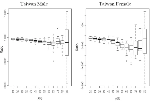
We shall first verify the regularity condition (4), and we use the ratio of life expectances in

Taiwan as a demonstration for checking the ratio

2 1 2 ) ( + + ⋅ n o n o n o e e e

. Figure 1 shows the boxplots for the

ratios of life expectancies in 1960-2005. The ratios are almost always smaller than 1, except for higher ages with fewer observations (and so larger fluctuations). Also, it seems that the ratios are a decreasing function of age and become level at higher ages. The ratios in U.S. show similar patterns.

Table 1. Life Expectancies of 6 Countries in 2000

Japan Sweden France England

& Welsh U.S. Taiwan

Male 77 77 75 74 74 74

Female 84 82 82 80 79 80

Figure 1. The Ratios of Life Expectancies in Taiwan

We shall first evaluate the ratios of numbers of survivors, using the inequality (2). Because the logarithms of mortality rates for the adult, except for the young adult, behave like a linear and

increasing function of age, the inequality 1

) ( 1 2 2 ≤ ⋅ + + n n n l l l

is equivalent top_n+1≤ p_x, which shall be true.

However, it should be noted that the mortality laws (e.g., the Gompertz law) are applied to calculate the mortality rates of very high ages in life tables. Thus, the ratios of numbers of survivors would rely on the methods of life construction and the inequality should be applied carefully. For

example, if the Gimpertz law is used, then ( 1) )

) log( exp( ) ( 2 2 1 2 = − − ⋅ + + _C C BCn n n n α α α is a decreasing

function of age and is always smaller than 1.

The ratios of life expectancies in Japan show different patterns (Figure 2). The ratios are very close to 1 for all adults except for the groups of ages 95 and over (smaller sample sizes). The ratios of life expectancies in Sweden, France, England & Welsh, and U.S. are between those in Taiwan and those in Japan. Among the six countries, Taiwan has the smallest life expectancies and Japan has the largest. This indicates that the life expectancy and the ratio of the life expectancies have some sort of connections. The ratios are close to 1 for countries with longer life expectancies. In the future, we shall collect data from countries with lower life expectancies and see

if the ratios are significantly smaller than 1.

Figure 2. The Ratios of Life Expectancies in Japan

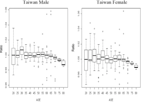
Figure 4. The Ratios of Mortality Rates in Taiwan

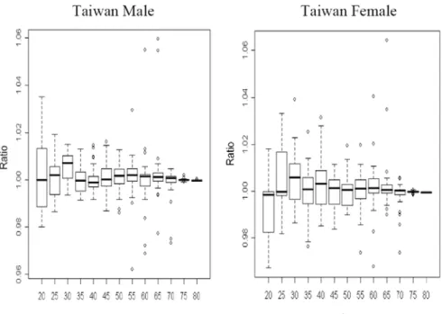
Next, we shall check the inequalities in (5) and (6). Figures 3 and 4 are the ratios of numbers of deaths and the ratios of the mortality rates in Taiwan. The ratios of numbers of deaths in Taiwan are very close to 1 as well, and they also decrease as the age increases. However, the ratios are not always smaller than 1, and they fluctuate around the value 1 and have larger ranges than those of the life expectancies. Similar patterns appear in the ratios of mortality rates (Figure 4). It should be noted that the mortality rates of ages 75 and over are derived via the Gompertz law and thus the ratios of mortality rates have very small ranges.

To double check the results, we also check the ratios of numbers of deaths and mortality rates in Japan. Figure 5 lists the ratios of numbers of deaths and mortality rates for the Japan male. The ratios also fluctuate around the value 1 and have larger variances, comparing to those of life expectancies in Figure 2. Similar results appear in the case of Japan female, as well as in Sweden, France, England & Welsh, and U.S. In other words, the ratios of life expectancies are close to 1 and also have smaller variances than those of numbers of deaths and those of mortality rates.

Figure 5. The Ratios of Numbers of Deaths Mortality Rates in Japan (Male)

Based on the empirical results, we found that the ratios of life expectancies satisfy the inequality (4) and that the ratios are closer to the value 1 for countries with higher life expectancies (such as Japan and Sweden). This indicates that the inequality (4) can serve as a possible constraint for regulating the mortality rates for the elderly. The ratios of numbers of deaths and mortality rates are also very close to 1 but have larger variances. However, the inequalities (5) and (6) are not always satisfied.

5. Discussions and Conclusions

In this study, we consider the discount sequence and introduce the concept into modeling the mortality rates of the elderly. We found that the frequently used mortality model (UDD, constant force, and hyperbolic assumption) and the Gompertz law all satisfy the regularity condition (2). But applying solely the condition (2) can only guarantee that px+1 ≤ px for the adult. This of

course can provide that some sorts of constraints to mortality rates. For example, in the LC model, the annual mortality improvement κ is usually a linear function of time, say, increasing function t

non-increasing function of age.

Since the inequality (2) provides a loose constraint for the mortality rates, we consider the inequalities (4), (5), and (6) to analyze empirical data from Taiwan, Japan, Sweden, France, England & Welsh, and U.S. Based on the life tables from these six countries, we found that the ratios of life expectancies are always smaller than 1 and countries with higher life expectancies have larger ratios. For both the male and female, Japan and Sweden have ratios of life expectancies almost equal 1. It seems that the ratios of life expectancies can serve a possible constraint for regulating the mortality rates. The ratios of numbers of deaths and ratios of mortality rates have similar behaviors but have larger variances. We suggest using the ratios of life expectancies to regulating mortality rates, instead of using those of numbers of deaths and ratios of mortality rates.

Although we found that the ratio of life expectancy can serve as a possible

constraint for smoothing mortality rates, there are some limitations in apply this inequality. First, the inequality can not be applied to modify mortality rates directly. The values of stationary populations (i.e., and ) are needed in computing the life expectancy. In other words, it is required to build a connection between the mortality rates and life expectancy. The other limit is that our empirical results depending on the life tables from six countries in this study. Different graduation and life table construction methods might give different results, although the UDD is usually assumed to compute the stationary population (i.e.,

2 1 2 ( + ) + ≤ ⋅ x o x o x o e e e x L Tx 2 1 1 0 + + + = =

_∫

x x t x x l l dt l L ).

Other than the six countries, we will consider other countries to make sure the result . If our conjecture is correct, countries with shorter life expectancies than Taiwan

and U.S. would have smaller ratio

2 1 2 ( + ) + ≤ ⋅ x o x o x o e e e 2 1 2 ) ( + + ⋅ x o x o x o e e e

, and countries with longer life expectancies than Taiwan

and U.S. would have ratio close to 1. Also, the inequality can not be applied

directly in modifying mortality rates. We shall consider other possible approaches to regulate the mortality rates, without relying too much on the life table construction methods. For example, the

2 1 2 ( + ) + ≤ ⋅ x o x o x o e e e

regular condition is also equivalent to i for o m m o i e q e

q ⋅ +1≤ ⋅ i≤m. We can try to modify this

References

z Berry, D.A. and Fristedt, B. (1985). Bandit Problems, Chapman & Hall.

z Brown, R.L. (1997). Introduction to the Mathematics of Demography, Society of Actuaries. z Cheung, S.L.K., Robine, J., Tu, E.J., and Caselli, G. (2006). Three dimensions of the survival

curve: horizontalization, verticalization, and longevity extension, Demography, 42(2), 243-258.

z Coale, A.J. and Kisker, E.E. (1990). Defects in data on old-age mortality in the United States: new procedures for calculating mortality schedules and life tables at the highest ages, Asian

and Pacific Population Forum, 4(1), 1-31.

z Kannisto, V. (1994). Development of Oldest-Old Mortality, 1950-1990: Evidence from 28

Developed Countries, Odense University.

z Kannisto, V. (2000). Measuring the compression of mortality, Demographic Research, vol. 3, Article 6.

z Lee, R.D. and Carter, L.R. (1992). Modelling and forecasting U.S. mortality. Journal of the

American Statistical Association, 87, 659–671.

z Olshansky, S.J. and Carnes, B.A. (1997). Ever since Gompertz, Demography, 34(1), 1-15. z Wilmoth, J. (1995). Are mortality rates falling at extremely high ages? An investigation based

on a model proposed by Coale and Kisker, Population studies, 49: 281-295.

z Wilmoth, J. and Horiuchi, S. (1999). Rectangularization revisited: variability of age at death within human populations, Demography, 36: 475-495.

z Yue, C.J. (2002). Oldest-Old mortality rates and the Gompertz law: A theoretical and empirical study based on four countries, Journal of Population Studies, 24, 33-57.