推挽式駐極體揚聲器之實驗建模與最佳化設計

國 立 交 通 大 學

機械工程學系

碩 士 論 文

推挽式駐極體揚聲器之實驗建模與最佳化設計

Experimental Modeling and Optimal Design of

Push-pull Electret Loudspeakers

指導教授：白明憲

研 究 生：王俊仁

推挽式駐極體揚聲器之實驗建模與最佳化設計

Experimental Modeling and Optimal Design of

Push-Pull Electret Loudspeakers

研 究 生： 王俊仁 Student：Chun-Jen Wang 指導教授： 白明憲 Advisor：Mingsian R.Bai 國立交通大學 機械工程學系 碩 士 論 文 A Thesis

Submitted to Department of Mechanical Engineering College of Engineering

National Chiao Tung University In Partial Fulfillment of Requirements

For the Degree of Master of Science

In

Mechanical Engineering July 2009

HsinChu, Taiwan, Republic of China.

推挽式駐極體揚聲器之實驗建模與最佳化設計

研究生：王俊仁 指導教授：白明憲 教授

國立交通大學 機械工程學系 碩士班

摘要

推挽式駐極體揚聲器是由輕、薄的駐極體材料製成的平面揚聲

器，但低頻響應的不足是其缺點。因此，搭配動圈式重低音系統可以

補償低頻響應的不足，組合成一套完整的音響系統。

本論文中利用電阻抗量測、曲線嵌合法以及質量增加法可以有效

鑑別出低音揚聲器單體的 T-S 參數。利用 T-S 參數以及機電聲類比電

路中，即可建立重低音揚聲器的集中參數模擬平台。藉由此平台可進

行反射式音箱的設計模擬，搭配約束最佳化方法可對音箱尺寸做最佳

化設計以提升低頻響應。

本論文亦對推挽式駐極體揚聲器進行分析與最佳化。本論文提出

一個完全利用實驗法對駐極體揚聲器建模的技術與駐極體揚聲器的

最佳化設計程序。因為駐極體揚聲器的電、機系統的耦合關係薄弱，

因此傳統利用電阻抗量測來進行參數鑑別的方法並不完全適用於此

揚聲器。因此，本論文發展了一套新的駐極體揚聲器實驗建模法，用

來鑑別駐極體揚聲器的電聲參數。利用雷射速度量測儀量測揚聲器的

振膜速度響應，進而鑑別出機械系統參數。搭配測試箱法，即可估測

電-力轉換因子與運動阻抗特性。利用此實驗鑑別法建立的模型可以

提供一個模擬平台，有效預測駐極體揚聲器的響應以及用於最佳化設

計。利用模擬退火法可計算出在多目標函數與多拘束條件下的最佳化

參數。不論對於多變數的廣泛求解或者只對於最佳間距的簡單求解都

可以藉由模擬退火法來達成。結果顯示最佳化設計可以有效提升駐極

體揚聲器的性能。

Experimental Modeling and Optimal Design

of Push-pull Electret Loudspeakers

Student: Chun-Jen Wang Advisor：Dr. Mingsian R.Bai

Department of Mechanical Engineering National Chiao-Tung University

Abstract

A push-pull electret loudspeaker is a flat type loudspeaker, and it is made with the thin and light electret material. The absence of low frequency response is a defect of the push-pull electret loudspeaker. Therefore, the subwoofer system is adopted to recover the low frequency response. The combination of the push-pull electret loudspeaker and the subwoofer can provide a complete audio system.

Via the electrical impedance measurement, the curve fitting and added mass method, the T-S parameters of the subwoofer can be identified. The conventional lumped parameter model of the subwoofer can be established using the EMA analogous circuit and T-S parameters. Next, the conventional lumped parameter model is employed to the simulation of vented-box system. The constrained optimization technology was also employed to find the design that can enhance the low frequency response of the vented-box system.

The push-pull electret loudspeaker is also analyzed in this thesis. A fully experimental modeling technique and a design optimization procedure are presented for push-pull electret loudspeakers. Conventional electrical impedance-based parameter identification methods are not completely applicable to electret speakers due to the extremely weak electromechanical coupling. This prompts the

development of a new experimental technique for identifying the electroacoustic parameters of the electret speakers. Mechanical parameters are identified from the membrane velocity measured using a laser vibrometer. The voltage-force conversion factor and the motional impedance are estimated, with the aid of a test-box method. This experimentally identified model serves as the simulation platform for predicting the response of the electret loudspeaker and optimizing the design. Optimal parameters are calculated by using the simulated annealing (SA) algorithm to fulfill various design goals and constraints. Either the comprehensive search for various parameters or the simple search for the optimal gap distance can be conducted by this SA procedure. The results reveal that the optimized design has effectively enhanced the performance of the electret loudspeaker.

誌謝

短短兩年的研究生生涯轉眼即逝。在此感謝白明憲教授的諄諄教誨與照顧， 在白明憲教授的指導期間，深刻的感受到教授對於追求學問的熱忱，更是佩服教 授淵博的學問與解決問題的方法。在教授豐富的專業知識以及嚴謹的治學態度 下，使我能夠順利完成學業與論文，在此致上最誠摯的謝意。 在論文寫作方面，感謝本系成維華教授和李安謙教授在百忙中撥冗閱讀，並 提出寶貴的意見與指導，使得本文的內容更趨完善與充實，在此學生致上無限的 感激。 在這兩年的研究生生涯中，承蒙博士班林家鴻學長、李雨容學姊，以及已畢 業的陳榮亮學長、劉青育學長、洪志仁學長、黃兆民學長、謝秉儒學長在研究與 學業上的適時指點，並有幸與郭育志同學、何克男同學、艾學安同學、劉冠良同 學互相切磋討論，讓我獲益甚多。此外學妹劉孆婷、學弟廖國志、廖士涵、陳俊 宏、張濬閣、桂振益、曾智文在生活上的朝夕相處與砥礪磨練，亦值得細細回憶。 因為有了你們，讓實驗室裡總是充滿歡笑。能順利取得碩士學位，要感謝的人很 多，上述名單恐有疏漏，在此一併致上我最深的謝意。 最後僅以此篇論文，獻給我摯愛的家人，祖父王德清先生、父親王天祺先生、 母親鄭淑櫻女士、二弟王俊淳以及三弟王鈺崇，這一路上，因為有你們的付出與 支持，給了我最大的精神支柱，也讓我有勇氣面對更艱難的挑戰。

TABLE OF CONTENTS

摘要...i

Abstract ... iii

誌謝...v

TABLE OF CONTENTS ...vi

LIST OF TABLES ... viii

LIST OF FIGURES ...ix

1. Introduction...1

2. Theory and Method...4

2.1 Electrical-mechanical-acoustical analogous circuit...4

2.2 The method of parameter identification ...7

2.2.1 Curve fitting method ...7

2.2.2 Added mass method ...8

2.3 Modeling acoustical systems ...9

2.3.1 Acoustic impedance ...10

2.3.2 Acoustic compliance ...10

2.3.3 Acoustic mass... 11

2.3.4 Radiation impedance of a baffled rigid piston ...12

2.3.5 Radiation impedance on a piston in a tube...13

2.3.6 Other acoustic elements ...14

2.4 Simulated annealing (SA) algorithm ...16

3. Modeling of Subwoofer ...19

3.2 Simulation and measurement of frequency responses...20

3.3 Optimal design of the vented-box system ...20

3.4 Simulation and measurement of vented-box design...21

4. Modeling of Push-Pull Electret Loudspeakers ...23

4.1 Operating principles ...23

4.2 Analogous circuits ...24

4.3 Parameters identification ...25

4.4 Numerical and experimental investigations ...28

4.5 Parameter optimization of electret loudspeakers...29

4.5.1 Optimizing the gap distance...29

4.5.2 Optimizing multi-parameters ...31

5. Conclusion ...33

LIST OF TABLES

Table 1. Acoustic resistance of a screen of area S ...38 Table 2. Experimentally identified lumped-parameters of a subwoofer...39 Table 3. Resulting obtained using the constrained optimization of vented-box system ...40 Table 4. Parameters of the optimized design versus the original non-optimized design. ...41

LIST OF FIGURES

Figure 1. (a) Electro-mechano-acoustical analogous circuit of loudspeaker (b) Same circuit with acoustical impedance reflecting to mechanical system ...42 Figure 2. The mechanical system of loudspeaker (M is diaphragm and voice coil mass, k is stiffness of suspension, C is damping factor)...43 Figure 3. (a) Detailed Electro-mechano-acoustical analogous circuit of loudspeaker (b) Another form of acoustic system ...44 Figure 4. (a) An acoustic resistance consisting of a fine mesh screen (b) Analogous circuit ...45 Figure 5. (a) Closed volume of air that acts as acoustic compliance (b) Analogous circuit ...46 Figure 6. (a) Cylindrical tube of air which behaves as acoustic mass (b) Analogous circuit ...47 Figure 7. Analogous circuit for radiation impedance on one side of circuit piston in infinite baffle...48 Figure 8. (a) Perforated sheet of thickness t having holes of radius a spaced a distance b (b) Geometry of the narrow slit ...49 Figure 9. Schematic diagram of vented-box system ...50 Figure 10. The overall EMA analogous circuit of vented-box using FEA-lumped hybrid method...51 Figure 11. T-circuit of transmission line ...52 Figure 12. (a) Front view of subwoofer (b)Back view of subwoofer ...53

Figure 13. The experimental arrangement for (a)measuring voice-coil impedance (b)measuring the on-axis SPL response...54 Figure 14. Simulated and measured frequency responses of the subwoofer. (a) the voice-coil impedance and (b) on-axis SPL response ...55 Figure 15. The impedance Z_AB of Vented-box ...56 Figure 16. Frequency response of optima vented-box design of subwoofer (a)Voice- coil impedance (b) On-axis SPL ...57 Figure 17. The push-pull electret loudspeaker. (a) Photo. (b) The configuration of the push-pull electret loudspeaker...58 Figure 18. The electroacoustic analogous circuits of the push-pull electret loudspeaker. (a) Electrical, mechanical, and acoustics systems. (b) Combined circuit referred to the electrical system...59 Figure 19. The electrical impedance measurement of the push-pull electret loudspeaker. (a) Experimental arrangement. (b) The electrical impedance versus the motional impedance. ...60 Figure 20. The comparison of the measured and simulated output voltage responses of the loaded and unloaded transformer. ...61 Figure 22. The membrane velocity measurement of the push-pull electret loudspeaker. (a) Experimental arrangement. (b) The comparison of the velocity responses of the loudspeaker, with and without the test box...63 Figure 23. The on-axis SPL measurement of the push-pull electret loudspeaker. (a) Experimental arrangement. (b) The comparison of the measured and the simulated on-axis SPL responses. ...64

Figure 24. The comparison of the measured THD of the electret loudspeaker between the push-pull and the single-ended configurations. ...65 Figure 25. The comparison of the on-axis SPL responses between the original and the optimal designs. (a) Results of optimizing only the gap distance. (b) Results of

optimizing four parameters including the gap distance, the resistance, the mass, and the compliance. ...66

1. Introduction

Loudspeakers are key components for many 4C (Computer, Communication, Consumer electronics, Cars) products. In this thesis, the subwoofer and push-pull electret loudspeaker will be discussed. The loudspeaker based on the electret technology is a flat type loudspeaker. The loudspeaker is made of thin and light electret material, which lends itself very well to space-concerned applications. However the absence of low frequency response is the defect of the electret loudspeaker. Therefore the subwoofer system is adopted to recover the low frequency response. The combination of the electret loudspeaker and the subwoofer can provide a complete audio system.

The subwoofer discussed in this thesis is primarily dynamic moving-coil type. The electroacoustic model of dynamic subwoofer involves electrical, mechanical, and acoustical domains. At the low-frequency regime, a loudspeaker can be modeled with electro-mechano-acoustical (EMA) analogous circuits and lumped parameters [1]-[4]. For dynamic loudspeakers, vented-box design has traditionally been used as a means for bass enhancement. Thiele [5], [6] and Small [7]-[10] have laid the theoretical foundation for vented-box design in a series of classical papers. Bai and Liao [11] applied the vented-box idea for designing acoustical enclosures of miniature loudspeakers for mobile phones. Along the same line, this thesis extends the previous idea to visualize the problem of interactions between the loudspeaker and the acoustical enclosure with a cavity and a port from a more universal and systematic perspective. The port and duct system is modeled as either a lumped mass or a transmission line.

Electret loudspeakers are the electrostatic loudspeakers with pre-charged membranes. Electret loudspeakers offer advantages of compactness, light weight,

excellent mid and high frequency reproduction, high electroacoustic efficiency, waiver of externally bias circuit, etc.[12] Due to these characteristics, the loudspeakers have promise in the application to consumer electronics.

Electret materials have been studied by several researchers. Lekkala and Paajanen [13] introduced a new electret material, ElectroMechanical Film (EMFi), at the turn of the century. Not before long, EMFi was applied to microphones, actuators and even loudspeaker panels.[14] Cao et al. [15] discussed the relationship between the microstructures and the properties of the electret material, where the electret properties of the porous PTFE (polytetrafluoroethylene) were studied. It is found that the porous dielectrics can be good electret materials. Recently, Chiang et

al. [16] proposed the nanoporous Telflon-FEP film that allows for higher charge

density stored in the film with improved stability. The nanoporous electret material was applied to flexible electrostatic loudspeakers.[17] Their electret diaphragms are made of fluoro-polymer with nano-meso-micro pores precharged by the corona method.

It was not until recently that Mellow and Kärräinen conducted a rigorous theoretical analysis of electret loudspeakers.[18]-[19] Transducers with single-ended and push-pull constructions are investigated in terms of the static force acting on the diaphragm and the stored charge density. Bai et al. suggested a hybrid modeling approach combining experimental measurement and finite-element-analysis (FEA) for a single-ended electret loudspeaker.[20] Experimental verification reported in the work revealed that the single-ended loudspeaker suffered from high nonlinear distortion problems.

This section aims at three purposes. First, electret loudspeakers in push-pull construction are proposed in order to reduce the nonlinear distortions encountered in the single-ended device. Second, a more accurate fully experimental modeling

technique is suggested to estimate the lumped parameters of the equivalent circuits without resorting to FEA. Because the coupling between the electrical and mechanical systems is extremely weak, the parameters of the mechanical system are unidentifiable using the electrical impedance measurement.[1]-[3] To overcome the difficulty, a test-box approach in conjunction with laser measurement is taken in this paper. Third, on the basis of the preceding simulation model, an optimization procedure using simulated annealing (SA) algorithm [21]-[23]is developed, aiming at optimizing design parameters of electret loudspeakers to maximize the SPL output and the bandwidth as well.

2. Theory and Method

A loudspeaker is an electroacoustic transducer that converts the electrical signal to sound signal. The processes of the transduction are complex. These cover the electrical, mechanical, and acoustical transduction. In order to model the process of the transduction, the EMA analogous circuit can be used to simulate the dynamic behavior of the loudspeaker. The circuit is overall and decomposed to electrical, mechanical, and acoustic part. A loudspeaker is characterized by a mixed of electrical, mechanical, and acoustical parameters.

2.1 Electrical-mechanical-acoustical analogous circuit

The concept of the electric circuit often applied to analyze transducers in the electrical and mechanical system. The technique analysis of the electric circuit can be adopted to analyze the transduction of the mechanical and acoustical system. The simple diagram of EMA analogous circuit is shown in Fig. 1. The subject of EMA analogous circuit is the application of electrical circuit theory to solve the coupling of the electrical, mechanical and acoustical system. The EMA analogous circuit is formulated by the differential equations of the electrical, mechanical, and acoustical system and the differential equations can be model by the circuit diagram. The rules of analytic methods are follows. For the electromagnetic loudspeaker, the diaphragm is driven by the voice coil. The voice coil has inductance and resistance which are defined R and _E L_E. The term R and _E are the most common

description of a loudspeaker’s electrical impedance. In order to model the

E

L

nonlinearity of inductance, a resistance R′ can be parallel connected to inductance. _E

Thus, the electrical impedance of loudspeaker is formulated as:

( // )

E E E E

When the current (i) is pass h e v ce coil, the f f ) is produced

and that drives the diaphragm

ed throug th oi orce (

to radiate sound. The voltage (e) induced in the voice coil when it movies with the mechanical velocity (u). The basic electromechanical equations that relate the transduction of the electrical and mechanical system are listed.

f =Bli (2)

Here, electro-m be modeled by a gyrator. So, the

loudspeaker im

e=Blu (3)

echanical transduction can pedance is formulated as:

2 E M MA Z Z i Z Z = = + + e Bl (4) where Z is the mechanical impedance and _M Z_MA is the acoustical impedance

reflecting in mechanical system as shown in Fig. 1 (b).

sim Th

agnetic loudspeaker. Force

( f ) is pro

p

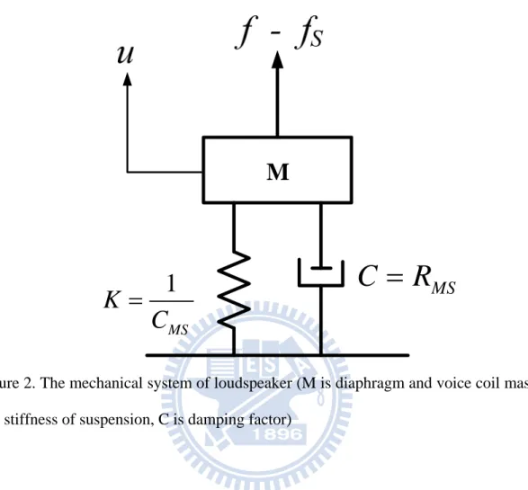
A ple driver model is shown in Fig. 2. is simple driver model can be

used to describe the mechanical dynamics of the electrom

duced according to the Eqs. (2). Vibration of the diaphragm of the loudspeaker displaces air volume at the interface. The primary parameters of the sim le driver are the mass, compliance (compliance is the reciprocal of stiffness) and damping in the mechanical impedance. The acoustical impedance is induced by the radiation impedance, enclosure effect and perforation of the enclosure. f is the _S

force that air exerts on the structure. The coupled mechanical and acoustical systems can be simplified as : MD M MS x M x= −f −R x_S − (5) f_S C

where M_MD is the mass of diaphragm and voice coil, f is the force in newtons,

S

f is the force that air exert on the structure, C_MS is the mechanical compliance,

MS

2 ( ) ( )( ) ( ) ( ) ( ) MD MS x s S MS M s j x s f s R j x s f C ω = − − ω − (6) ( ) ( ) ( ) ( ) ( ) MD MS S u s MS M s j u s f s R u f j C ω ω = − − ( _{M A}) ( ) s − f = Z +Z u s (7) where _{M MD MS} 1 MS Z j M R j C ω ω

= + + is the mechanical impedance and Z is the _A

acoustical impedance.

S A

f =Z u (8) The acoustical impedance primarily includes radiation impedance, enclosure impedance, and perforation of the enclosure. The acoustical impedance can be formulated as:

A AF AB

Z =Z +Z (9)

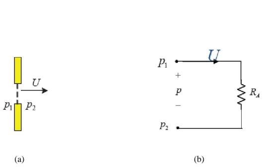
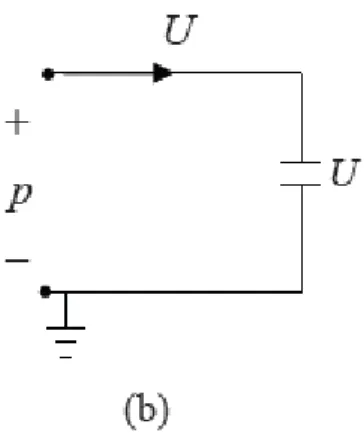
The general acoustic circuit is shown in Fig. 3 (a). The Z_AF means the

impedance in the front of diaphragm and Z_AB means that in the back side. In general, the circuit would turn to Fig. 3 (b) the general form in the electronics. The following discussion will use this kind of circuit.

The two basic variables in acoustical analogous circuit are pressure p and volu

pressure

me velocity U. Because of using impedance analogy, the voltage becomes

p and current becomes volume velocity . Therefore, the ground of

this circuit showing in Fig. 3 means the pressure of the free air. Thus, it also can U

employ the concept about the mechanical system and the acoustical system can be coupled by the below two equations.

S D f =S p 0) U =S u (11) The equation (1 D S D

f =S p represents the acoustic force on the diaphragm

generated by the difference in pressure between its front and back side, where S_D is the effective diaphragm area and p is the difference in acoustic pressure across the

D

U =S u

diaphragm. The volume velocity source represents the volume velocity

emitted by the diap

front and rear of the diaphragm is given by

hragm. From the Eqs. (10), the pressure difference between the

( _{AF AB}) p=U Z +Z parame owe res to calcula (12) Usin 11), force

Almost all of the useful loudspeaker ters had been defined by other

researchers before Thiele and Small. H ver, Thiele and Small made these

The added mass m curve fitting metho

ass of the iaphragm will induce the alteration of the onant frequency. The curve fitting arameters of Thiele and Small

used te and the result is more

accurate.

g Eqs. (10) and ( field can be transformed to pressure field.

2.2 The method of parameter identification

parameters in a complete design approach and shown how they could be easily determined from impedance data.

ethod (Delta mass method) and d are

chosen to calculate the Thiele and Small parameters. Modifying the m d

employs the impedance of system to calculate the p

precisely. Both methods are explained in the following section.

2.2.1 Curve fitting method

The curve fitting method is Q _ES

The procedure of the curve fitting method is explained as follows.

(a) Choose the ( 1 )

j M R 1

j C

ω

ω

+ + to be become the basic element that it fit a

peak of the impedance curve. Because the purpose of the method is to fit the mechanical part, the electrical part can be obtained previously.

the fitting range in the im dance curve. If the range of the

roadly, result of the fitting is poor. Therefore, the

(b) Choose pe

range that starts and ends both sides of peak enclo es the peak, and it can be chosen. Then, the peak will fit better and it is obtained second order syste

sur

m transfer function.

(c) We compare the coefficient between the second order transfer function and

2 2

2 1

s s

s + ξω ω+ , then the parameters ωs and QMS are solved.

2 s fS ω = π 1 MS Q 2ξ = (13) ( E ) ES ES MS R Q Q R = (14)

2.2.2 Added mass method

added mass can be written as

The resonance frequencies of the subwoofer diaphragm without and with the

1 n A A M C ω = (15) ' 1 ( ) n A A A M + ΔM C ω = , (16)

where ΔM_A denotes the added mass expressed in the acoustical domain, M_A and

A C sim denote aco ltaneously for ustical mas u

s and compliance, respectively. Solving Eqs. (15) and (16)

A M and C_A yields ' 2 2 1 1 1 CA A n n M ω ω Δ _{⎝ ⎠} ⎛ ⎞ = _⎜ − _⎟ (17) 2 1 A M = nCA ω (18)

This corresponds to the mechanical mass and compliance

2 MS A D M =M S (19) 2 A MS D C C S = , (20)

D

S

where i

the nominal area). Finally, the motor constant (Bl) and the mechanical resistance

s the effective area of the loudspeaker diaphragm (approximately 60% of

(R_MS) can be estimated as follows:

E S MS ES R Bl C Q ω = (21) S MS MS MS M R Q ω = (22) And the lossy voice-coil inductance can be calculated, using the following method:

( ) ( )n E E Z jω ≈ jω L ' cos( / 2) n e E L R nπ ω ⎡ ⎤ = ⎢ ⎥ ⎣ ⎦ , 1 cos( / 2) n e E L − L ω nπ ⎡ ⎤ = ⎢ ⎥ ⎣ ⎦ (n=1:indu (23) ctor; n=0:resistor)

The parameters n and L can be determined from one measurement of _e Z_VC at a frequency well above f , where the motional impedance can be neglected _s

E VC E Z =Z −R 2 1 1 2 1 ) ln ln E ln ln Im( ) 1 tan 90 Re( E Z Z Z n Z _⎦ ω − ω − ⎡ ⎤ − = _{⎢ ⎥}= ⎣ ， E E n Z L ω = (24)

The method to calculate lossy voice-coil inductance is described [20].

Electroacoustics is usin the analogous circuit to model the acoustical behavior including acoustic mass, acoustic resistance and acoustic compliance. The impedance type of analogy is the preferred analogy

sound pressure is analogous to voltage in electrical circuits. The volume velocity is analogous to current.

2.3 Modeling acoustical systems

g

2.3.1 Acoustic impedance

Acoustic resistance is associated with dissipative losses that occur when there is a viscous flow of air through a fine mesh screen or through a

The capillary tube. Fig. 4(a) illustrates a fine mesh screen with a volume velocity U flowing through it.

1 2

p= p −p , where p is the ₁

pressure difference across the screen is given by

pressure on the side that U enters and p is the pr₂ side that exits.

The pressure difference is related to

essure on the U

the volume velocity through the screen by

1 2 A

p p p R U (25)

where _A

= − =

R is the acoustic resistance of the screen. The circuit is shown in Fig. 4(b).

Theoretical formulas for acoustic resistance are generally not available. The values are usually determined by experiments. Table 1 gives the acoustic resistance of typical screens as a function of the area S of the screen, the number of wires in the screen, and the diameter of the wires.

2.3.2 Acoustic compliance

To illustrated an acoustic compliance, consider an enclosed volume of air as illustrated in Fig. 5(a). A piston of area is shown in one wall of the enclosure.

Acoustic compliance is a parameter that is associated with any volume of air that is compressed by an applied force without an acceleration of its center of gravity.

When a force

S

f is appli to the piston, it moves and compresses the air. Denote the

piston displacement by ed

x and its velocity by u . When the air is compressed, a

restoring force is generated which can be written f =k x_M , where k is the spring _M

constant. (This assumes that the displacement is not too large or the process cannot be modeled with linear equation.) The mechanical compliance is defined as the reciprocal of the spring constant. Thus we can write

1

M

M M

x

f =k x= =

∫

udt (26)

This equation involves the mech

C C

anical variables f and . We convert it to one that involves acoustic variables

u

p and U by writing f = pS and u=U S/

to obtain 2 1 1 M A p=

∫

Udt=

∫

Udt (27) S C C

This equation defines the acoustic compliance C of the air in the volume. It is _A

given by

2

A M

C =S C (28)

An integration in the time domain corresponds to a division by jω for phasor variable. It follows from Eqs. (27). That the phas re is rela to the phasor volume velocity by

or pressu ted

A

p U

j Cω

= . Thus the acoustic impedance of the compliance is 1

A

A

p

Z = = (29)

The impedance which varies inversely with

U jwC

jω is a capacitor. The analogous circuit is shown in Fig. 5(b). The

to gr

li onnect e ground

e acoustic compliance of the volume of air is given by the expression derived for the plane wave tube. It is

figure shows one side of the capacitor connected ound. This is because the pressure in a volume of air is measured with respect to

zero pressure. One node of an acoustic comp ance always c s to th

node. Th 2 A C c V ρ = (30)

2.3.3 Acoustic mass

Any volume of air that is accelerated without being compressed acts as an acoustic mass. Consider the cylindrical tube of air illustrated in Fig. 6 (a) having a length l and cross-section S. The mss of the air in the tube is M_M =ρ₀Sl. If

the air moved with u, the force required is given by f M_M du dt

= . Th

velocity e

volume velocity of the air through the tube is U =Su and the pressure difference

between the two ends is p p₁ p₂ f

S

= − = . It ws from these relations that the

pressure difference

follo

p can be related to the volume velocity U as follows:

1 2 2 M M A M du M dU dU p= p −p = = =M (31) where S dt S dt dt A

M is the acoustic mass of the air in the volume that is given by

0 2 M A l M S S M = = ρ (32)

A differentiation in the time domain corresponds to a m ltiplication by u jω for sinusoidal phasor variable. If follows from Eqs. (31) that the phasor pressure is

related to the phasor volume velocity by p= j M Uω _A . Thus the acoustic

impedance of the mass is

A A

p

Z = = j M (33)

An electrical impedance which is proportional to

U ω

jω

isfy

is an inductor. The analogous circuit is shown in Fig. 6(b). For a tube of air to act as a pure acoustic

e velocity. . Oth

mass, each particle of air in e tube must move with the sam This is

strictly true only if the frequency is low enough erwise, the motion of the air particles must be modeled by a wave equation. An often used criterion that the air in the tube act as a pure acoustic mass is that its length must sat

th

8

l≤λ , where λ is the wavelength.

Radiation imp nce

vibra otio

2.3.4 Radiation impedance of a baffled rigid piston

eda can be easily explained by an example of the diaphragm

tion. When the diaphragm is vibrating, the medium reacts against the m n of the diaphragm. The phenomenon of this can be described as there is impedance

between the diaphragm and the medium. The is called the radiation impedance.

impedance

The detail of the theory of radiation impedance is clearly described by Bernek. The analogous circuit of the radiation impedance for the piston mounted in an infinite baffle is shown in Fig. 7. The acoustical radiation impedance for a piston in an infinite baffle can be approximately over the whole frequency range by the analogous circuit. The parameters of the analogous values are given by

0 1 2 8 3 A a M ρ π = (34) 0 1 2 A R a 0.4410ρ c π = (35 ) 0 2 A R a2 c ρ π = (36) 3 1 2 0 where 5.94 A a C c ρ = (37) 0

ρ is the density of air, c is the sound speed in the air, is the radius of the circuit piston.

only used to model the diaphragm of a direct-radiator loudspeaker when the e

as that for the piston in an infinite b

circuit is given in Fig. 7. Th

a

2.3.5 Radiation impedance on a piston in a tube

The flat circuit piston in an infinite baffle that is analyzed in the preceding section is comm

nclosure is installed in a wall or against a wall. If a loudspeaker is operated away from a wall, the acoustic impedance on its diaphragm changes. It is not possible to exactly model the acoustic radiation impedance of this case. An approximate model that is often used is the flat circuit piston in a tube.

The analogous circuit for the piston in a long tube is the same from

affle; only the element values are different. The analogous e parameters of the analogous values are given by

1 0.6133 a A M ρ π (38) = 1 2 a 0.5045 A c R ρ π (39) = 2 2 A c R a ρ π = (40) 2 3 1 A 2 0.55 a C c π ρ = (41)

2.3.6 Other acoustic elements

A. Perforated sheets

Perforated sheets are often used as an acoustic resistance in application where an acoustic mass in series with the resistance is acceptable. Fig. 8 (a) illustrates the geometry. If the holes in the sheet have centers tat are spaced more than on diameter

apart and the radius a of the holes satisfies the inequality 0.01 a 10

f f < < ,

where f is the frequency and a is in m, the acoustic impedance of the sheet is

given by 2 0 t a a ρ ⎧ ⎡ ⎛ π ⎞⎤ ⎫ 2 2 2 1 2 1.7 1 A Z u j t N aπ ω a ω ⎡ ⎤ ⎪ ⎛ ⎞ ⎪ b b = _{⎨ ⎢} + _⎜ − _⎟⎥+ _⎢ + _⎜ − _⎟⎥⎬ ⎝ ⎠ ⎣ ⎦ ⎝ ⎠⎦ ⎪⎭ ⎪ ⎣ ⎩ (42)

where N is the number of holes. The parameters μ is the kinematic coefficient of viscosity. For air at 20 C° and 0.76 mHg, 1.56 10 m5 2

s

μ _{≈ ×} −

. This parameter value app oximately as r T1.7

0

P , where perature and is the

atmospheric pressure.

A tube having a very small diameter is another example of an acoustic element which exhibits both a resistance and a mass. If the tube radius in meters satisfies

T is the Kelvin tem P ₀

a 0.002

a

the inequality

f

0 4 2 4 ' 8 A l l Z j 3 a a ρ η _ω π π = + (43)

where l is the actual length of the tube and l' is the length including end

corrections. The parameter η is the viscosity coefficient. For air,

5_{N S} − ⋅ ° 0.7 2 1.86 10 m

η at and 0.76 . This parameter varies with

temperature as , where e Kelvin tem ure. If the radius of the tube

= × 20 C

T

mHg

p

T is th erat

0.01 _a 10 _{, the acoustic impedance is given by}

satisfies the inequality

f f < < 0 0 2 2 ' 2 2 A l l Z u j a s a ρ _{ω ω} ρ π π ⎛ ⎞ = _⎜ + _⎟+ ⎝ ⎠ (44) 0.002 _a 0.

For a tube with a radius such that 01

f < < f , interpolation must be

used between the two equations.

A narrow slit also exhibits both acoustic resistance and mass. Fig. 8 (b) shows t of the slit in meters satisfies the inequality

the geometry of such a slit. If the heigh t

0.003

t

f

< , the acoustic impedance of the slit, neglecting end corrections for the mass term, is given by

0 3 12 5 A l l Z η j ρ t ω + ω ωt (45)

B. Vented-box system

s shown in Fig. 9.

SP with radius aP and length LP. The mechanism of low-frequency enhancement lies

in the Helmholtz resonator comprised of the acoustic mass in the vent and the

nce c

istance. ss of

the port and acoustic compliance of the encl =

The general diagram of a vented-box system i The system

primarily consists of an enclosure of volume VAB and a port with a cross-sectional area

acoustic complia in the en losure. More precisely, the vent can be modeled as an

acoustic mass and an acoustic res The acoustic resistance, acoustic ma

0 2 2 2 P ABP P P L ρ ⎡ ⎤ R a ωμ a π = _⎢ + _⎥ ⎣ ⎦ (46) 0 ABP P P M L S ρ = . (47) 2 AB AB V C = (48)

The m pedance obtained using FEA mentioned above is changed into

a lumped-parameter model.

0c ρ

echanical im

Therefore, the overall EMA analogous circuit of vented-box is shown in Fig. 1

odel of a duct

0.

C. Transmission line m

The vent also can be modeled as a transmission line model. Consider a length of duct, the equivalent-circuit model for the transmission line is the T-circuit shown in Fig. 11. These equations of T-circuit are in transfer matrix form as follows [22], [40]. 2 1 2 1 1+ 2 1 a a a b b a b b Z Z Z p 1 p Z Z ⎡ ⎤ _{⎝ ⎠} ⎡ ⎤ + ⎢ ⎥ where U _Z U Z Z ⎡ ⎛ ⎞⎤ + ⎢ ⎜ ⎟⎥ ⎢ ⎥ = ⎢ ⎥ _{⎢ ⎥}⎢ ⎥ ⎣ ⎦ ⎣ ⎦ ⎢ ⎥ ⎣ ⎦ , (49) 0tan( ) 2 P a kL Z = jZ (50) 0 sin b P Z Z j kL = (51) 0 0 P c Z S ρ ≡ , (52) e k is wave number,

wher L is length of vent. _P

2.4 Simulated annealing (SA) algorithm

The SA algorithm is a generic probabilistic meta-algorithm for the global optimization problem, namely, locating a good approximation to the global optimum

of a given function in a large search space. The major advantage of the SA is the ability of avoid becoming trapped in the local minima. In the SA method, each state in the search space is analogous to the thermal state of the material annealing process. The objective function G is analogous to the energy of the system in that state. The purpose of the search is to bring the syste

generated state with the minimum objective function. An improve state is accepted If the objective function is decreased, the new state is always accepted. If the objective function is increased and the following inequality holds, the new state will be accepted: [23]

m from the initial state to a randomly

in two conditions. exp( G) P T γ Δ = − > , (53)

where P is the acceptance probability function, ΔG is the difference of objective function between the current and the previous states, T is the current system

perature, and γ

tem is a random number which is generated in the interval (0,1). In

to accept a new state that is “worse” than the present one. This m

the high temperature T, there is high probability P

echanism prevents the search from being trapped in a local minimum. As the annealing process goes on and T decreases, the probability P becomes increasingly small until the system converges to a stable solution. The annealing process begins at the initial temperature T and proceeds _i

with temperature that is decreased in steps according to

1 k k T₊ αT , (54) where 0 1 = α

< < is a annealing coefficient. The SA algorithm is terminated at the preset final temperature T . In the electret loudspeaker optimization, we choose _f

1000

i

T = , T_f = ×1 10−9, and α =0.95. Next, two design optimization problems will be examined. The first problem concentrates on only optimizing the gap distance d between the membrane and the electrode plate, whereas the second

problem attempts to optimize four design parameters: the gap distance d, the compliance C , the mass _M′ M , and the resistance _M R . _M

3. Modeling of Subwoofer

3.1 EMA analogous circuit of subwoofer

A sample of moving-coil subwoofer with a 12 cm diameter is shown in Fig. 12. The front and rear view of the subwoofer are shown in Figs. 12 (a) and (b), respectively. The EMA analogous circuit of this subwoofer can be established in Fig. 3. The coupling of the electrical domain and the mechanical domain is modeled by a gyrator, whereas the coupling of the mechanical domain and the acoustical domain is modeled by a transformer [3]. The T-S parameters can be identified via electrical impedance measurement [3], as summarized in Table 2. The dynamic response of the subwoofer can be simulated on the platform of this model.

Thus, the Loop equations can be written as follows:

0 0 0 1 E g ms D D D AF D 0 Z Bl i e Bl Z S u S Z P ⎡ ⎤ ⎡ ⎢₋ ⎥ ⎢ ⎢ ⎥ ⎢ ⎢ − ⎥ ⎢ ⎣ ⎦ ⎣ ⎤ ⎡ ⎤ ⎥ ⎢ ⎥₌ ⎥ ⎢ ⎥ ⎥ ⎢ ⎥ ⎦ ⎣ ⎦ , (55)

where i is the current, u is the mean velocity of the diaphragm, _D S is the effective _D

area of the diaphragm, e is the driving voltage, s_g = jω is the Laplace variable, and ' ( || ) E E E E Z =R + R L s (56) 1 2 1 1 1 = || || AF A A A A Z R R M C s ⎛ ⎞ + ⎜ ⎟ ⎝ ⎠ s (57)

The symbol “||” denotes parallel connection of circuit. The loop equations can be solved for the current and velocity of the diaphragm for each frequency. From the current and velocity, the electrical impedance and the on-axis SPL responses of the subwoofer can be simulated.

3.2 Simulation and measurement of frequency responses

Simulations and experiments are undertaken in this thesis to validate the aforementioned integrated subwoofer model. The frequency response from 3 Hz to 20 kHz of the subwoofer is measured using a 2.83 Vrms sweep sine input. Figure 13 (a) shows the experimental arrangement for measuring voice-coil impedance (with symbols defined in the figure):

s vc g s e Z R e e = − (58)

Figure 13 (b) shows the experimental arrangement for measuring the on-axis SPL response by using a microphone positioned at 10 cm away from the subwoofer.

Using Eqs. (59) and (60), the voice-coil impedance and SPL can be simulated. Figures 14 (a) and (b) compare the voice-coil impedance and the on-axis SPL obtained from the simulation and the experiment, respectively. It can be observed that response predicted by conventional lumped parameter model is in good agreement with the measurement.

g vcs e Z i = (59) (dB) 20* log( ) 94 2 jkr D D e SPL j S u r ωρ π − = + (60)

3.3 Optimal design of the vented-box system

As mention in section 2.3.6 previously, the vented-box design can be adopted to reach the goal of bass enhancement. The design variables are selected to be the port radius (a ), the duct length (_P L ) and the volume of cavity (_P ). The Helmholtz frequency of the vented box system is selected to be 30Hz. To initiate the SQP constrained optimization procedure, the lower resonance frequency of the coupled speaker-enclosure system is also selected to be 30 Hz. The design variables are

AB

V

mass modeling the vent can be modeled as a transmission line model. The cost function is chosen as the maximum sound pressure level at the frequency 30Hz. This can be written in terms of the following optimization formalism:

3 2 5 10 a 5 10 1 3 2 5 1 2 5 6 1 1 10 1.5 5 10 9 10 1 10 1 10 max SPL( , , ) st. 1 10 2 10 1 10 2 10 30 ( ) 0 P P AB A P P AB A A M L V M a L V R C f r − − 1 − − − − − − − ⎪ _{× ≤ ≤} ⎪ ⎪ × ≤ ≤ × ⎪ × ≤ ≤ × ⎪ ⎨ × ≤ ≤ × ⎪ ⎪ × ≤ ≤ × ⎪ = ⎪ ⎪ _{Δ =} ⎩ ⎧ × ≤ ≤ × (61)

where MA , RA are CA areobtained from acoustic system resistance. The circuit of the impedance Z_AB is shown in Fig. 15. Thus, the impedance Z_AB in Fig. 3 can be obtained. The loop equations can be written as follows:

1 2 0 0 0 0 0 0 1 0 0 1 0 1 0 ( ) 0 0 0 0 0 E D g ms Z ⎢ ⎢ D⎥ D AF AB C D ABP a b ABP a b b AB D D b b a b B Bl Z u e Bl S u S Z j C u i S R Z Z R Z Z Z j C P S Z Z Z Z Z ω ω ⎡ ⎤ ⎥ − ⎡ ⎤ ⎡ ⎤ ⎢ ⎥ ⎢ ⎥ ⎢ _{⎥ ⎢ ⎥ ⎢ ⎥} − ⎢ _{⎥ ⎢ ⎥ ⎢ ⎥=} ⎢ _{⎥ ⎢ ⎥ ⎢ ⎥} ⎢ _{⎥ ⎢ ⎥ ⎢ ⎥} + + − − − − − ⎢ _{⎥ ⎢ ⎥ ⎢ ⎥} ⎣ ⎦ ⎣ ⎦ ⎢ ⎥ ⎢ _{− + +} ⎥ ⎣ ⎦ (62) The results obtained using constrained optimization are also summarized in Table 3.

ement of vented-box design

tained previously using constrained optim

3.4 Simulation and measur

A mockup was made for validating the vented-box design ob

ization. The frequency response from 3 Hz to 20 kHz of the subwoofer is measured using a 2.83 Vrms sweep sine input. Fig 16 (a) and (b) the voice-coil impedance and the on-axis SPL with the vent open are compared, respectively. The solid line is the result of simulation. The dot is the result of

experiment. The result of SPL response reveals that the resonance frequency of couple speaker-enclosure system is at 20 Hz which is lower than initial design. The SPL at 20Hz is about 92 dB. The goal of bass enhancement can be achieved.

4. Modeling of Push-Pull Electret Loudspeakers

4.1 Operating principles

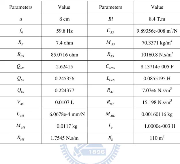
A sample of a electret loudspeaker is shown in Fig. 17(a).

In its push-pull construction, the loudspeaker comprises a charged flexible membrane and two perforated rigid back plates with 52.1% perforation ratio. The membrane is made of fluoro-polymer which contains nano-pores to enhance the charge stability and density.[17] The membrane is placed at the center between two electrode plates spaced by 2.4 mm, as shown in Fig. 17(b). The construction is also referred to as the push-pull configuration with a fully-floating membrane by Mellow et al.[19] The membrane is divided into six equal partitions (

493 mm 129 mm×

242 mm 37 mm× ) by stainless steel spacers.

Due to high input impedance of the electret loudspeaker, a transformer with turn-ratio 125 is used for impedance matching and e_spk is the output voltage of the transformer. The net force f acting on the membrane can be estimated by [19]

2 2 1 1 2 3 1 0 1 2( ) 2 ( ) r r m r r m spk spk r r r r hS h S f e e d h d h ε ε σ ε ε σ _{δ φ κ} ε ε ε ε ε = + = + + + δ where , (63) and ε_r1 vely r

ε are the relative permittivities of the membrane and the medium at

the gap, respecti , ε₀ is the vacuum permittivity, h is one half of the thickness of the membrane, SD is the area of membrane, σm is the surface charge density of the

membrane, d is the gap between the membrane and the electrode plate, and δ is the displacement of the membrane. The first term of Eq. (63) is due to the input voltage, whereas the second term is due to the negative stiffness resulting from the m brane attractions. The voltage-force conversion factor

em

φ and the negative stiffness κ can be written as [19] 1 2 K d φ = , r1 r h d ε ε (64)

with 1 2 hS 1 r m r K ε σ ε = , and 2 3 K d κ = , r1 r h ε d ε (65) with 2 2 1 2 2 0 2 r m r h S K ε σ ε ε =

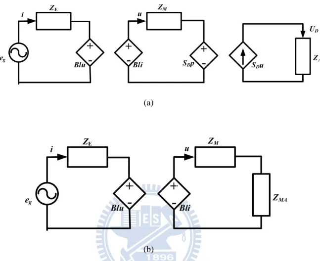
4.2 Analogous circuits

The electret loudspeaker can be modeled with the analogous circuit, as shown in al domain, the circuit is modeled with the Thévenin equ

.

Fig. 18(a). In the electric

ivalent circuit, where e is the voltage source of the transformer input, i is the _in

current, R and _E L are the electric resistance and inductance of the transformer. _E

E

C is the static capacitan when the membrane is blocked. In the mechanical ce

domain, Z_M ts the open-circuit mechanical impedance and is the

ustical domain,

represen u

membrane velocity. In the aco Z represents the acoustical _A

imp

systems are reflected to the electrical system, where the motional impedance edance.

Figure 18(b) shows the combined circuit as the mechanical and acoustical

mot Z is defined as 2 2 mot Z_ms S Z_{D A} Z = + , (66) φ 1 2 ( ) ms M E C Z jω Z φ = + , (67) where _ms −

Z is the short-circuit mechanical impedance and ω is the angular

frequency To measure the electrical impedance, we need an experimental arrangement, as shown in Fig. 19(a). The input voltage from the signal generator

.

g

e is 1.5 V and the current-sampling resistor R is 100 ohm. The electrical

1 2 g R spk e G G e R Z = − R, (68)

ere G and ₁ G denote the effective gains of the amplifier and the transformer, ₂

respectively, and e is the voltage drop _R e

wh

across the resistor R. The thus measured electrical impedance of Fig. 19(b) resembles that of a capacitance due to weak electro-mechanical coupling9

1

( )

E E

Z = C − . (69)

It follows that on the static capacitance C can be extracted from the electrical _E

impedance measurement ω ly 1 ( ) E E C = ω Z − (70)

For the sample in Fig. 17

4.3 Parameters identification

ductance of the transformer output end is connected to the electret loudspeaker

d order low-pass system. respo se of the unloaded transformer, which is nearly -20k Hz. As the electret loudspeaker is connected to the transformer, the frequency response becomes a low-pass function with cutoff frequency

, the C was found to be 1.86 nF. _E

E

L

n 20 In Fig. 18(b), as the in

which behaves like a capacitance due to the aforementioned weak coupling, the combined electrical system becomes a 2n

Figure 20 shows the frequency constant throughout the range of

0 E ω = 8736.4 Hz: 2 2 1 1 1 1 ( ) 1 spk in in in E E E E s s C L s C R s Q ω ω + + _{+ +} 0 0 ( ) ( ) ( ) ( ) ( ) E E E e s =H s e s = e s = e s (71)

where H(s) is the transfer function between _{spk in E}

and s j

e and e , Q is the quality factor

ω

= is the Laplace variable. The effective inductance and resistance at the output end of the transformer can be calculated by

2 1 0 ( ) E E E L = ω C − , (72) . (73) At the resonance frequency, the real part of the transfer function in Eq. (71) is zero.

1 0

( )

E E E E

R = Q ω C −

It follows that the quality factor can be calculated by

0

( _E ) _E

H jω = −jQ =Q_E. (74)

For the sample in Fig. 17, the quality factor = 0.6845, the inductance =

0.178 H and the resistan

E

Q L_E

ce R = 14.3k ohm, respectively. In Fig. 20, the _E

measurement (solid line) and the simulation (dash-dot line) of e_spk are in good agreement.

As mentioned previously, the

mechanical measurement. To this end, the electrical and acoustical systems are reflected to the mechanical system, as shown in Fig. 21(a). For simplicity, we

im system. The lumped parameters

mechanical parameters are unidentifiable with the electrical impedance measurement. We need to devise a method based on direct

approximate the combined acoustical impedance and the mechanical pedance to be

a 2nd-order R , _M M_M and C′_M denote the

sis

re tance, the mass and the compliance, respectively, of the combined impedance. Due to weak coupling (φ ≈ ), 0 R_Eφ2 and L_Eφ2 can be neglected, leading to the simplified circuit of Fig. 21(b). Solving the circuit yields the expression of the membrane velocity u 0 2 0 0 1 1 1 1 M in in u s C s u e e s M C s R C s R Q 2 ( ) ( ) ( ) 1 u M M M M M Q s ω φ φ ω ω = = + + _{+ +} , (75)

where the compliance C_M is the series combination of C′_M and the negative

compliance 2

/

E

C φ

quality factor. The membrane velocity can be measured by a laser vibrometer, as shown in Fig. 22(a). In the following, we concentrate on only the fundamental mode and ignore higher-order modes. From the velocity measurement, t

resonance frequency

he fundamental

0

ω can be located and the quality factor corresponding to the fundamental resonance can be estimated:

0 2 1 u

Q = ω

ω ω− , (76)

where the ω₂ and ω₁ are -3dB points in the velocity response.

Given the ω₀ =1/ M C_{M M} , it is impossible to determine the respective values of the compliance C and the mass _M M based on one measurement. To overcome _M

the difficulty, a test box method with volume 5.51 L is employed to obtain another velocity measurement. The result of the membrane velocity measurement is shown in Fig. 22(b). The

500 Hz due to the acoustical compliance of the test box. Based on these two membrane velocity measurements, the mechanical parameters can be determined:

fundamental resonance frequency is increased from 315 Hz to

2 ) 0 0 [( B 1] M M C ω C ω Δ , (79) = − , (77) 2 1 M = C − , (78) 1 0 M u 0 ω ( ) M M ( _M) R = ω Q C − 2 2 ( E) M M E M C C C C C φ φ ′ = , (80) +

where ω_{0 B} is the fundamental resonance frequency of the velocity response when loaded with the test box and ΔC_M is the additive mechanical compliance due to the test box. Finally, the voltage-force conversion factor φ can be determined by

0

ω ω= in Eq. (75): letting

0 ( ) M in R u e ω φ = , (81)

where u(ω₀) is the peak magnitude of the membrane velocity response at the fundam ntal resonance frequency. Using the formula, e φ is found to be 1.88 10× −4 for the sample in Fig. 17.

eriments were conducted to validate the preceding model of the electret loudspeaker. The experimental arrangement for measuring the on-axis sound pressure level (SPL) is shown in Fig. 23(a). According to the standard AES2-1984

itioned 1 m away from the loudspeaker.

Figure 23(b) compares the on-axis SPL responses obtained using the simulation ) is in good agreement with the m

4.4 Numerical and experimental investigations

Exp

(r2003) [24], a 2475 mm 2025 mm× baffle is used in the measurement. The

132.6 Vrms swept-sine signal is used to drive the loudspeaker in the frequency range 20-20k Hz. The microphone is pos

and the measurement. The simulated response (solid line

easured response (dashed line), albeit discrepancies are seen at high frequencies due to un-modeled flexural modes of membrane. It should be borne in mind that, in the preceding model, only the fundamental mode is modeled in the analogous circuit and high-order modes are neglected.

It can also be observed from Fig. 23(b) that the SPL response starts to roll off at approximately 8k Hz due to the inductance of the transformer as predicted. Furthermore, in Fig. 19(b), the motional impedance obtained using the model is much greater than the electrical impedance, rendering the former an open circuit in Fig. 18(b). This is the evidence of weak coupling.

For assessing the nonlinear distortion of the electret loudspeaker, THD is calculated from the measured on-axis SPL response [25]. In Fig. 24, the measured

THD of the electret loudspeaker in push-pull construction is compared with that of the singl

p distance

In the section, only the gap distance that is easiest to alter in making a mockup e net attraction force actin

off frequency will also become lower (because of the increased static apacitance) as the gap is decreased.

o increase the attraction force until the displ

e-ended construction which was investigated by Bai et al.[20] The average THD of the push-pull configuration is below 6% in the range of 140-20k Hz, while the THD of the single-ended configuration can reach as high as 17%. Evidently, the push-pull configuration has effectively addressed the nonlinearity problem of the single-ended configuration.

4.5 Parameter optimization of electret loudspeakers

The preceding model of electret loudspeaker serves as a useful simulation platform for optimizing the loudspeaker parameters. In the following, a procedure based on the simulated annealing (SA) algorithm [21]-[23] is exploited for the design optimization.

4.5.1 Optimizing the ga

will be optimized. If all other conditions remain unchanged, th

g on the membrane and hence the SPL output will increase as the gap is decreased. However, the gap can not be decreased indefinitely, or else, stick-up condition of the membrane and the electrode plates can occur. Another issue is that the upper

roll-c

As we keep decreasing the gap t

acement of the membrane equals the gap distance, we call this distance the critical gap distance. Only dynamic distance need to be concerned since, at the quiescent state, the static attraction forces due to resident charges in the membrane are balanced with the push-pull construction. Membrane displacement can be can be

obtained by integrating the velocity expression in Eq. (75) 1 2 0 0 1 ( ) in M u e K u Q δ ω = = + + , (82) 2 0 1 ( ) 1 u s s s R Qω d ω

when the peak value of the displacement

where 2

1/

K d

φ = in Eq. (64) has been invoked. The collision condition occurs

max

gives the critical gap distance

δ is equal to the gap distance d. This

1/ 3 2 1 0 u in M u _u Q K d∗ e ⎧ ⎫ ⎪ ⎪ = ⎨ ⎬ ⎪ ⎪ ⎩ ⎭ . (83) 2 0.25 R Qω _{Q −}

In the experiment, the driving signal is a 132.6 Vrms swept sine. That corresponds to a critical gap distance 0.19 mm, which also represents an upper bound of displacement for the following optimization. Figure 25(a) compares the SPL responses for various gap distances (including the critical gap). Clearly, the SPL is

. H

reased static capacitance.

In order to find a compromise solution between the original design and the design with the critical gap, the SA algorithm is employed alongside the preceding increased if the gap distance is decreased owever, this comes at the expense of decreased bandwidth due to inc

simulation model for finding the optimal gap distance. Two goals are set up for the design optimization. It is hoped that the SPL in the range of 800-5k Hz is maximized while maximizing the upper roll-off frequency, i.e.,

2 1 new 1 1 N n N = 2 uc G = f , (SPL ( )) , ( ) [800 Hz,5k Hz], 1, , G =

∑

n f n ∈ n= … N , (84) (85) where SPL_new is the current SPL response, n is the frequency index in the range of

800-5k Hz, and f is the upper -3dB cutoff frequency of _uc SPL_new. The compound objective function G_TG can be written as

1 2

1 1

TG

G = + ×w , (86)

where w is a weighting constant (w = 0.23 in the simulation).

G G

In addition, the design variable (gap distance) and the associated constraints are gi

following inequalities: ven in the max (mm)<d (mm) 0.4 (m δ ⎧⎪ ⎨ ⎪⎩ (87)

With the SA procedure, the optimal gap distance is found to be 0.86 mm, which enhances the average SPL by approximately 5 dB, as shown in Fig. 25(a).

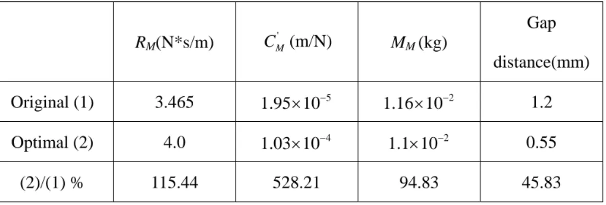
4.5.2 Optimizing

multi-m)< <d 3.6 (mm)

parameters

In the section, we shall extend the preceding one-parameter optimization to more comprehensive optimization for four parameters: the gap distance, the resistance R , _M

the mass M , and the com_M pliance C′_M. Apart from the level and the upper cutoff design goals, a third goal of the lower cut-off is added to the objective function:

, (88)

3 lc

G = f

where f denotes the lower -3dB cutoff frequency of _lc SPL_new. The compound objective function G_TM reads

1 2 1 2 1 1 TM G w w G G G = × + × + 3, (89)

50000 in the simulation. The design varia

where the weights w = 2400 and ₁ w = 1₂

3 1 6 ' 4 N s N s 0.698 ( ) 69.8 ( ) 1.4 10 ) M M R M ⋅ ⋅ ⎧ _{≤ ≤} ⎪ × ≤ ⎪ ⎪ max (mm d (mm) δ < ⎪ ⎪⎩

The results of optimization using the SA algorithm are summarized in Table 4.

m m (kg 1.43 10 (kg) m m 1.95 10 ( ) 1.95 10 ( ) N 0.12 (mm) 12 (mm) ) M C d − − − − ⎪ ≤ × ⎪ _{× ≤ ≤ ×} ⎨ ⎪ ≤ ≤ ⎪ ⎪ (90) The design with optimized parameters is simulated in Fig. 25(b). The lower cutoff frequency of the optimal design (circled mark) has been decreased from 315 Hz of the original design to 150 Hz as the mechanical compl

average SPL is enhanced by about 12 dB as the gap is decreased to 0.55 mm.

N

5. Conclusion

A push-pull electret loudspeaker is a thin, light and flat loudspeaker and it is very suitable to using in space-concerned applications. However, the absence of low frequency response is a defect of the push-pull electret loudspeaker. Therefore, the subwoofer system is adopted to recover the low frequency response. The combination of the push-pull electret loudspeaker and the subwoofer can provide a complete audio system.

The EMA analogous circuit is employed to establish a conventional lumped parameter model of the subwoofer. Via the electrical impedance measurement, the curve fitting and added mass method, the T-S parameters of the subwoofer can be identified. Using the platform, the electrical impedance and the on-axis SPL responses of the subwoofer can be simulated. The response predicted by conventional lumped parameter model is in good agreement with the measurement. Next, the conventional lumped parameter model is employed to the simulation of vented-box system. The constrained optimization technology was also employed to find the design that can enhance the low frequency response of the vented-box system.

The push-pull electret loudspeaker is also analyzed in this thesis. A fully experimental modeling technique and an optimization procedure have been developed for push-pull electret loudspeakers. The experimental modeling technique relies on not only the electrical impedance measurement but also the membrane velocity measured by using a laser vibrometer. With the aid of a test box, the voltage-force conversion factor and characteristics of motional impedance can be identified from the membrane velocity. The experimentally identified model serves as the simulation platform for optimizing the design parameters of the electret loudspeaker.

The SA algorithm was exploited to find the parameters that yield optimal level-bandwidth performance. Either only the gap distance or the comprehensive search for various parameters can be optimized by using the SA procedure. The results reveal that the optimized design has effectively enhanced the performance of the electret loudspeaker, as compared to the original design.