國 立 交 通 大 學
機械工程學系
博士論文
穩定與指向機構之研究
Design for Stabilizer and Pointing Mechanism
研 究 生:游 武 璋
指 導 教 授:成 維 華 教授
中 華 民 國 九 十 六 年 七 月
穩定與指向機構之研究 研究生 :游 武 璋 指導教授: 成 維 華 教授 國立交通大學機械學系 摘 要 本論文由機構自由度的觀點設計機載感測裝置,進而發展出六自 由度運動平台搭配空中載具,使置於其上之雙軸感應器環架能穩定完 成其指向之位置,並利用工作空間分析規劃機載內外空間。 在飛行器上為了使感測器能穩定指向其視線並補償飛機飛行時 所產生誤差,因此需要設計環架控制機構與六自由度的穩定器。環架 機構可使感測器能完成指向功能,而六自由度穩定器則用於即時補償 飛行器所產生的運動誤差,使得感測器能穩定的完成工作。 雙軸環架機構之討論包含精密之轉動區塊環架機構設計、機構最 佳化設計、機械效能分析﹔而位置補償平台之分析包含平台工作空間 重建與分析、靈巧度分析、工作空間最佳化。並利用邊界方塊技術來 分析機構工作空間得到更詳盡三度空間圖形資料使得工作空間可被 更精確估算。 ii
Design for Stabilizer and Pointing Mechanism
student: Wu-Jong Yu Adviser: Dr.Wei-Hua Chieng Department of Mechanical Engineering
National Chiao Tung University
Abstract
In this dissertation, we discuss the design of the airborne sensor
hardware architecture based on the degree freedom perspective. The six
D.O.F. motion base is therefore developed and placed beneath the two-axis sensor gimbal to compensate the air vehicle motion error, and stabilize the pointing direction. In addition we use the technique of the workspace analysis to layout the inside and ouside space of the airborne vehicle.
In order to stabily point the sensor into the commanded line-of-sight and to compensate the motion error derived from the aircraft flight, the gibmal control with the mechanism design and the six degree-of-freedom stabilizaer are needed. The gimbal mechanism is used for the function of pointing, and the six degree-of-freedom motion platform is used for the motion compensation induced by the flight vehicle, therefore the sensor can be stabiliy perform its task.
The two-axis gimbal design includes a precise mechanical gimbal
design for the turning block, the mechanical optimization design, and the mechanical advantage analysis.
The platform analysis of the position compensation includes iii
workspace reconstruction technology, workspace analysis, and dexterity analysis with optimization. The marching cube technology is used for the workspace analysis and estimation with the detailed 3D graphic data for more accurate evaluation for the workspace.
誌 謝 感謝最支持我的指導老師成維華,有機會讓我從工業工程與技職 體系的背景,拔擢接觸正統機械領域。老師包容我的無知和大膽,使 得跨領域創造出許多非正規的結果,但老師卻諄諄善誘讓我有機會了 解進而謹慎,數年來的督促與指導,使我獲益良多,並使得本論文得 以完成。 感謝每位口試老師精闢的指教與見解,真的感恩,使得本論文更 加完善。 感謝我的父母親與家人在我最沮喪的時候,給予我最大的支持。 感謝我未婚妻思育無怨無悔的支持,陪伴著我攻讀博士班的日子。 感謝至方學長的鞭策指導包容,讓我能完成許多難以克服的難關。 感謝學弟永成、家豐、仰宏、裕都分擔許多計畫和推導。 感謝領航賴董事長、學長建勳、俊旭、同事們兩年來的包容。 感謝過去教導我的陳福春、張敏德、施志雄、駱景堯……。 最後感謝所有在這期間曾經支持我的所有人,謝謝你們。 v
Contents
摘 要………..ii Abstract……….………..…...…………..……….iii 謝 誌……….v Contents……….…..…...……….……….vii List of Figures……….…………..ix List of Tables……….………..xii CHAPTER 1 INTRODUCTION...1CHAPTER 2 BUILDING BLOCK APPROACH TO PARALLEL MANIPULATOR DESIGN...5
2.1 Reviews...5
2.2. Gr¨uebler's criterion ...6
2.2.1 Joint ...7
2.2.2 Limb: Dyad, Triad, and Quad ...8
2.2.3. Open chain...9
2.2.3. Parallel manipulator ...10
2.3 Parallel manipulator design synthesis...11
2.3.1 Fully-symmetric, parallel manipulator (FSPM)...12
2.3.2 Semi-symmetric, parallel manipulator (SSPM)...13
2.3.3 Task-oriented, parallel manipulator (TOPM) ...14
2.3.4 Saturated limb ...14
2.4 Design Synthesis by building blocks...15
2.4.1 FSPM/SSPM/TOPM ...15
2.4.2. Ground vs. floating actuator...16
2.4.3. Selection of active limb...16 vi
2.4.4. Selection of passive limb ...17
2.4.5. Insertion of saturated limb ...17
2.5 Design Examples of 3-dof TOPM ...18
2.5.1. Parallel manipulated Cartesian machine ...18
2.5.2 Parallel manipulated wobble machine ...18
2.5.3 Parallel manipulated rotation machine...19
2.5.4 Parallel manipulated cobra-head machine ...19
2.6 Design Examples of 6-dof TOPM ...19
CHAPTER 3 DESIGN OF THE SWINGING-BLOCK AND TURNING- BLOCK MECHANISM WITH SPECIAL REFERENCE TO THE MECHANICAL ADVANTAGE ...21
3.1 Reviews...21
3.2 Swinging-Block and Turning-Block Mechanisms ...22
3.3 Maximum Average Mechanical Advantage...23
3.4 Optimal Design ...26
3.5 Design Procedure...28
CHAPTER 4 ROBOTIC SAFEGUARD SYSTEM AND WORKSPACE ANALYSIS...30
4.1Reviews...30
4.2 The Active Multi-Robotic Safeguard System Architecture...33
4.3 The Robot System Installation and the Kinematics Analysis...35
4.4 The Robotic Operation and Control Interface Program ...37
4.5 The Robot Language Programming for the Safeguard System...38
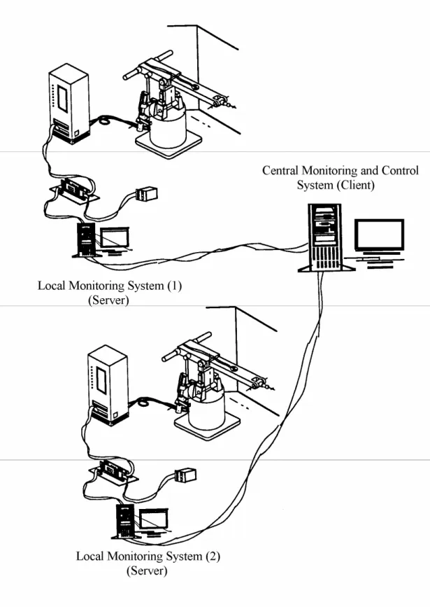
4.6 Client-Server Networking Architecture...41
4.6.1 Client ...42
4.6.2 Server...42
4.7 Robot Remote Supervision (Case One)...45
4.8 Virtual Reality Remote Supervision for Safeguard of Robotics (Case Two) ...46
CHAPTER 5 WORKSPACE AND DEXTERITY ANALYSES OF THE STABILIZER (DELTA HEXAGLIDE PLATFORM) ...48
5.1 Reviews...48
5.2 Delta Hexaglide Platform ...50
5.2.1 Inverse Kinematics...50
3.2.2 Dexterity Analysis...53
5.3 Marching Cube Method...57
5.3.1 Workspace Presentation ...58
5.3.2 Workspace Examples ...59
5.4 Analysis and Design...60
5.4.1 Combination of Workspace and Dexteriy Analysis...61
5.4.2 Dimensional Design ...62 CHAPTER 6 CONCLUSION...64 Reference………..………70 Figures………...……….………..79 Tables...………...………130 viii
List of Figures
Figure 1. Vehicle and Sensor relation ...79
Figure 2. Sensor, Gimbal, stabilizer, air cushion...79
Figure 3. The limb...80
Figure 4. SS triad ...80
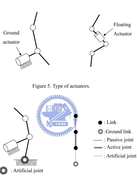
Figure 5. Type of actuators ...81
Figure 6. (a) Kinematic structure (b) corresponding graph...81
Figure 7. Reduced graph of parallel manipulation ...82
Figure 8. (a) Tripod-based PKM (b) Stewart platform (Hexapod)...82
Figure 9. Example of a 5-dof SSPM...83
Figure 10. DDB measurement as Saturated limb ...83
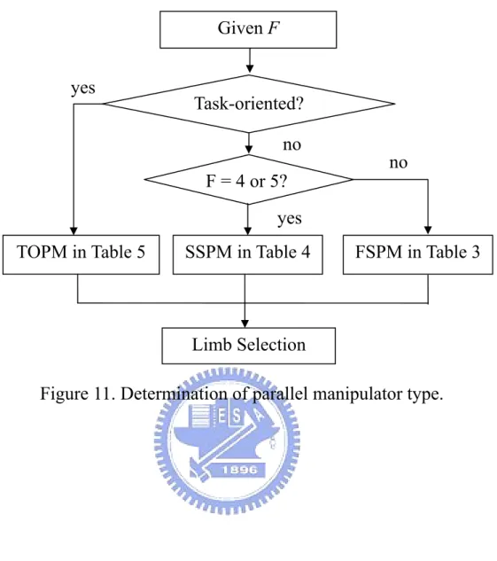
Figure 11. Determination of parallel manipulator type ...84
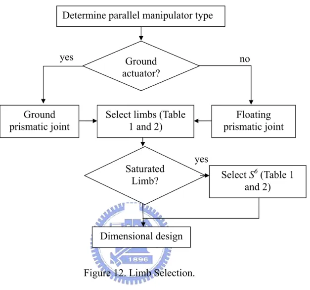
Figure 12. Limb Selection ...85
Figure 13. Cartesian machine ...86
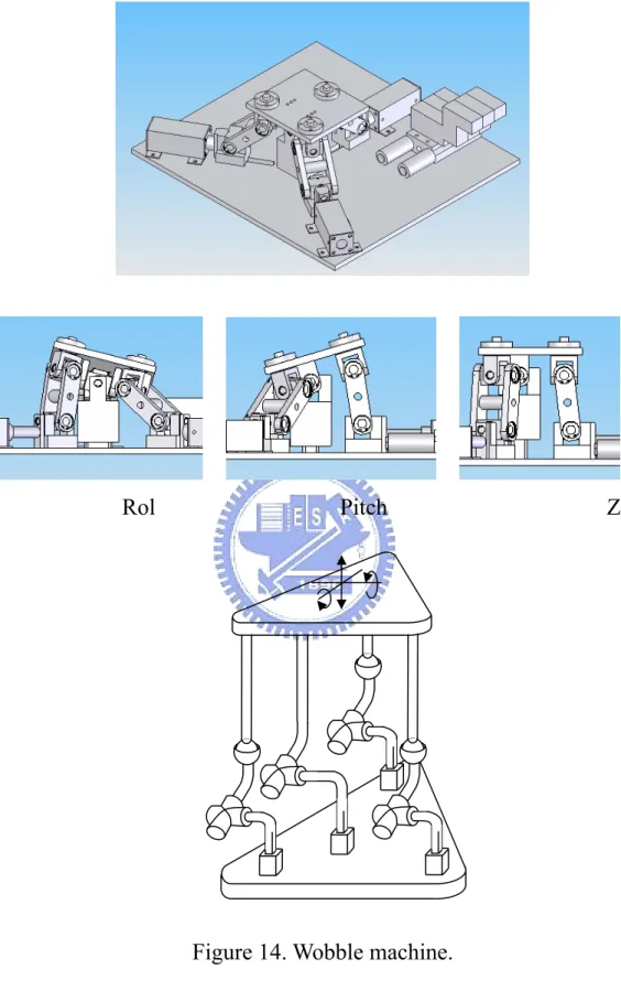
Figure 14. Wobble machine ...87
Figure 15. Rotation machine...88
Figure 16. Cobra-head machine...88
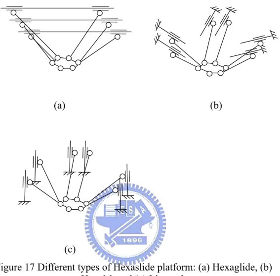
Figure 17. Different types of Hexaslide platform: (a) Hexaglide, (b) HexaM, and (c) Linapod ...89
Figure 18. Delta Hexaglide platform ...89
Figure 19. (a) Kinematic structure and (b) photograph of the Delta Hexaglide platform mechanism (Courtesy: IMON Inc.) ...90
Figure 20. Oscillating-cylinder engine mechanism...91
Figure 21. RRRP kinematics inversion...91
Figure 22a. The real sensor pedestal picture ...92
Figure 22b. Kinematic structure of turning-block mechanism...92 ix
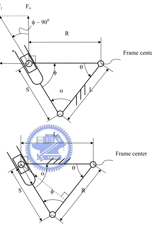
Figure 23. Force transmitted and kinematic structure of (a) Turning-block
and (b) Swinging-block mechanism...93
Figure 24. Dimensional design for turning block mechanism ...94
Figure 25. Example of turning-block illustrated configuration...95
Figure 26.
ε
versus D/R and ε versusη
...96Figure 27.
ε
versus R/L versusθ
...96Figure 28. The active Multi-Robotic safeguard system arichitecture ...97
Figure 29. The coordinate system for the robotic collision detection ...98
Figure 30. The industrial U-type robot ...99
Figure 31. The Parallel-linked robot system...100
Figure 32. The interface program for the industrial robot...101
Figure 33. The networking for the industrial robot controller interface.102 Figure 34. The industrial robot control interface display ...103
Figure 35. The Levels of robot safe range...104
Figure 36. Interpretative process of LEX & YACC. ...105
Figure 37. The interpretative process of setting safe-range...106
Figure 38. Programming construction of NETCOMM ...107
Figure 39. Three-Layer architecture (Service Model)...108
Figure 40. (a) The tester application program ...109
(b) The frame maker window of tester...109
Figure 41. Java's applet of robot in case one ...110
Figure 42. Architecture of robot supervision (Case One)...111
Figure 43. Architecture of virtual reality remote supervision for safeguard of robotics (Case Two) ...112
Figure 44. The photograph of the two-robot system ...113
Figure 45. The network delay for the different size of the transmitted data between two robotic controllers ...114
Figure 46. The network delay for the different size of the transmitted data among multiple robotic controllers ...115 Figure 47. Top and front view of the Delta Hexaglide platform ...117 Figure 48. Dexterity of the Delta Hexaglide platform...118 Figure 49. Graphical presentation of (a) the voxel with one center and (b)
the cube with eight vertices ...119 Figure 50. Surface representation in Marching Cube method...119 Figure 51. 15 unique cube configurations ...120 Figure 52. The translational workspace of Delta Hexaglide at α = 0, β = 0,
γ = 0; 16416 faces are found on the boundary; 24775 cubes are found inside the workspace. ...121 Figure 53. Workspace degeneracy: (a) workspace island (in dotted circle), and (b) workspace cavity (in dotted circle)...123 Figure 54. The parking position...124 Figure 55. Combination of workspace and dexterity result of the Delta
Hexaglide; shape complexity is 0.446 and workspace Volume is 5568. ...125 Figure 56. Different designs of the Delta Hexaglide platform ...126 Figure 57. (a) Workspace Volume and (b) Shape Complexity of the
translational workspace via different L...127 Figure 58. (a) Workspace Volume and (b) Shape Complexity of the
translational workspace via different rupper...128
Figure 59. (a) Workspace Volume and (b) Shape Complexity of the
rotational workspace via different L ...129
List of Tables
Table 1. List of spatial triads ...130
Table 2. List of spatial quads ...130
Table 3. The classes of limb used in the spatial FSPM ...131
Table 4. The classes of limb used in the spatial SSPM ...131
Table 5. The classes of limb used in the spatial TOPM ...132
Table 6. Dimensional parameters used in examples; L is varying from 3.15 to 3.40 in Figure 12.and 13. ...132
Table 7. Thirty-seven normal directions (vectors) of different patches for surface representation in marching cubes ...133
Table 7.1 Definition of patch-in-a-Cube based on the edge sequence number...134
Chapter 1 Introduction
There are two types of motion errors that require compensation in air vehicles with stabilizers. The first type comprises orientation motion errors induced by atmospheric disturbance and maneuvering. Sensors, such as a TV camera, E-O/IR, radar, or even a gun, on an air vehicle must be kept stable for constant pointing orientation during flight. The ground stabilization command can be expressed as:
I B I B C u u = , (1.1) where B =[
ϕ
][θ
][ψ
], I C A [ E][ A] B C =σ
σ
][
σ
E and [σ
A] are antenna elevation and azimuth angles,respectively, installed on the aircraft body axis, and [
ϕ
], [θ
], and]
[
ψ
are roll, pitch, and roll Euler angles, respectively, where uB is theunit vector of the aircraft body axis, anduI is the unit vector of the
line-of-sight for the sensor pointing direction in the inertial space. Conversely, for image radar, such as synthetic aperture radar [1], the second motion error is line-of-sight range deviation between the antenna phase center of the air vehicle and the target map patch center. The deviation range decreases map resolution and quality, and requires compensation; this compensation is called motion compensation (MOCOMP) [2]. The along-track (line-of-sight (LOS)) range deviation-induced phase error (Fig. 1) can be calculated as follows:
∫
− = VLOSdt LOSλ
π
φ
4 (1.2) 1where VLOS is the LOS range deviation,
λ
is the wavelength of the radar transmission wave, and dt is the radar pulse repetition interval (PRI).Conventionally, the first motion error type can be overcome with the sensor gimbal controller using inertial sensor data, and the second motion error type can be compensated by electronic phase adjustment, either in real time or non-real time.
This work introduces a novel six D.O.F.(degree of freedom) motion base [3] placed beneath the gimbal, which plays the role of a type-I (orientation) motion error stabilizer and a type-II (translation) [motion compensator OR MOCOMP]. The advantages of the new approach for motion stabilization and compensation are as follows.
1. The motion base provides high pointing accuracy and rapid frequency response due to the better stiffness of the inherent parallel mechanism characteristics.
2. A sensor gimbal typically only has two D.O.F.. The proposed stabilizer is a good solution for compesating for type-I errors.
3. The MOCOMPfor image radar can be compensated for by the
motion base directly, without need for any electronic phase adjustment, as long as the LOS range deviation is within the workspace of the motion base translational movement.
High frequency vibration is removed using an air cushion system [4] such as passive or active shock mounts. With the autopilot enabled, the remaining middle and low frequency errors, such as orientation error, flight-path error, or flight-speed error, can be compensated for by the six D.O.F. platform. Figure 1 presents the relationhip between the sensor and the air vehicle.
In this dissertation, we presents a methodology for parallel manipulator design. The parallel manipulators are categorized into fully-symmetric, semi-symmetric, and task-oriented types. According to these types, different limbs may be chosen for building the desired parallel manipulator. Useful limbs including the dyad, triad, and quads
are enumerated for individual selections in the design process. The
task-oriented, parallel manipulator is found particularly useful for performing tasks applicable to the domain of high speed machining. Following this design methodology, the linkages and joints are decided as shown in Fig. 2 which is a new six D.O.F. motion base as the motion stabilizer and compensator.
The direction pointing equipment for airborne sensors is a two-axis gimbal. The two-axis design uses low power, is lightweight, has a small volume and high strength structure, has a minimal number of linkages, and generates maximal output force. With the proposed actuator, the turning block as the natural gearbox structure is used for the two-axis gimbal to acquire mechanical design limits. The turning block and swing block mechanical advantages, and the mechanical optimization of the gimbal [5] are analyzed.
The gimbal stabilizer is a Delta Hexaglide Platform. The platform consist of two plates, six linkages, and six sliders as shown in Fig. 19. The upper plate is a “moving plate” which is an end-effector with six D.O.F.. The other plate, which is fixed on ground, is called a “fixed base;” however, it is now fixed on the vehicle air cushion.
The stabilizer system is designed in light of vehicle space
limitations and safety issues. This work considered robot safeguards with virtual boundary techniques [6], and other space adjustments,
using virtual reality (VR) programming to determine workspace boundaries. Therefore, the stabilizer must be rebuilt in a three-dimension Cartesian space using the VR technique. The dexterity problem can be verified and the platform design optimized.
Chapter 2 Building Block Approach to Parallel
Manipulator Design
2.1 Rewiews
The Stewart/Gough platform, the most well-known platform manipulator, is a 6-dof platform controlled by six active prismatic joints [7]. Six UPS limbs connect the fixed base to the moving platform. Applications of parallel manipulators are commonly found in the motion platform for pilot training simulators, positioning devices for high precision surgical tools, parallel-type multi-axis machining tools and precision assembly tools.
The design on trajectory planning and application developments
of parallel manipulators are challenging due to the closed-loop nature.
Analysis work include the generation of and forward pose solution for analytic parallel manipulators [8], parallel manipulator dynamics [9], singularity determination in spatial platform manipulators [10], and inertial measurement unit calibration [11].
Advanced manufacturing will involve application of new concepts, models, methodologies, and information technologies. Because of this recent trend towards high-speed machining, there is also a demand to develop machine tools with high dynamic performance, improved stiffness and reduced moving mass. Parallel manipulator has been adopted to develop this type of machine. Design and analysis work corresponding to a particular parallel manipulator called parallel kinematic machine (PKM) [12]-[14] has been
introduced.
Referring to the reconfigurable parallel robots, the kinematic design of modular reconfigurable in-parallel robots [15], the conceptual design of a modular robot [16], and the CMU reconfigurable modular manipulator system [17] have been presented. Toward the structural synthesis, the structure synthesis of a class of 4-D.O.F and 5-D.O.F parallel manipulators [18] and the qualitative synthesis method for 3-D.O.F and 4-D.O.F parallel manipulators [19] have been uncovered. As to the design synthesis of task-oriented modular parallel robots, the scientific methodology for matching tasks to modular robot [20] and the methodology for design of parallel mechanisms based on the application of graph theory and combinatorial analysis [21] have also been introduced.
Many methods have been developed for the analysis and design synthesis of parallel manipulators. However, the structural synthesis of parallel manipulators in general has not been attempted. This chapter introduces a general aspect of parallel manipulator design. Some innovated task-oriented parallel manipulators with 3-D.O.F. will also
be introduced.
2.2. Gr¨uebler's criterion
Gr¨uebler's criterion calculates the theoretical number of D.O.F
within a mechanism. This is also known as the mechanism's F number.
D.O.F is the number of independent joint variables which must be specified in order to define the position of all links within a mechanism. A body restricted to planar motion has at most three
D.O.F. The link is a rigid body. The joint is a contact (or permanent
connection) between two links. The number of links may be denoted by l. The number of joints may be denoted by j. The type of joint (or connection) defines the relative motion of the two connected links.
There are five categories of contacts in spatial motion, they allow for fj
D.O.F between the connected bodies, where 1≤ fj ≤5. A fj = 6
contact would be a non-contact. The theoretical D.O.F F within a mechanism calculated by the Gr¨uebler's criterion is expressed as follows.
∑
+ − − = l j fj Fλ
( 1) (2.1)where λ is the mobility of the space in which the mechanism
operates (λ = 3 for general plane mechanism, λ = 6 for spatial mechanism). The number of independent loops of the mechanism is denoted by L. According to Euler’s formula it is obtained that L = j – l + 1. The above equation is then written into
∑ −
= f L
F j
λ
(2.2)The above equation is useful in mechanism synthesis design when the number of independent loop usually indicates the complexity of the mechanism.
2.2.1 Joint
An artificial joint, joint with no D.O.F ( = 0), is introduced in this chapter for the following derivations. The joints with
are then called the normal joints. The joints connect the links can be revolute (f
j
f
5
1≤ fj ≤
j = 1), prismatic (fj = 1), cylindrical (fj = 2), universal (fj = 2)
or spherical joints (fj = 3). Higher order joints with fj > 3 may be
composed by the lower order joints fj ≤3. The high order joints may
not be generally useful in the parallel manipulators for their difficulty in fabrication. In this chapter, we will look only into the joints
with . The normal joint attached with an actuator is called the
active joint; on the other hand, it is called the passive joint. 3
≤
j
f
2.2.2 Dyad, Triad, and Quad
The F number within a mechanism calculated by the Gr¨uebler's criterion is provided with the existence of a ground link. The mobility ground link is subtracted from the overall F number. In case that the kinematic structure is floating with respect to the ground, the mobility
M of the kinematic structure may be derived from Gr¨uebler's criterion
as ∑ + − = l j fj M
λ
( ) (2.3)A particular floating kinematic structure with L = j – l + 1 = 0 is called the limb as shown in Fig. 3.
The mobility of the limb is derived from eq. (2.3) that ∑
+
= ji
i f
M
λ
, (2.4)where ∑ fj,i denotes the total number joint D.O.F on the ith limb.
The limb with one joint connecting two links is called a dyad. The limb with two joints in series connection to three links is called a triad. The limb with three joints in series connection to four links is called a quad. For convenience, the total number of D.O.F of the joints is denoted by T that
∑
= fj
T . (2.5)
The total number of joint D.O.F of the ith limb, according to eq. (2.4), is derived as
λ
+ = TM (2.6)
In order to avoid the under-constraint condition of the Gr¨uebler's criterion, the limb should have the total joint D.O.F T no more than λ. Otherwise, there will be either an uncontrollable rotation or an uncontrollable translation in the limb. The limb with T = λ is called the saturated limb. The ambient space of a saturated limb is the space in which the mechanism operates.
Table 1 lists some of the useful spatial (λ = 6) triads using the
aforementioned joints. The term “class” i.e. sT, in Table 1 is used to
denote the class of limbs with total joint D.O.F of the limbs equal to T. In Table 1, the SS triad, as shown in Fig. 4, is a saturated limb, however, there is an uncontrollable rotation between two spherical joints. The uncontrollable rotation presents as an under-constraint of the Gr¨uebler's criterion.
Table 2 lists some of the useful spatial (λ = 6) quads using the aforementioned joints.
In order to classify limbs, we define the limb embodying an active joint the active limb; it is a passive limb if no actuator is attached. Different versions of actuators are shown in Fig. 5. The actuators being connected to the ground are called ground actuators; others are called the floating actuators.
2.2.3. Open chain
A limb is defined as the limb with one end grounded. A convenient way to represent an open-chain is the graph representation as shown in Fig.6
In the analysis point of view, the ambient space of the open-chain 9
is given by the Cartesian product of the joint spaces of all the joints that make up the open-chain [22].
2.2.3. Parallel manipulator
A parallel manipulator as shown in Fig. 7 is regarded as a set of limbs connected in parallel to a common rigid body, known as the end-effector. The reduced graph may be expanded into individual graphs representing different limbs.
Let an integer n denote the number of limbs, an integer li denote
the number of links of the ith limb respectively, and an integer ji
denote the number of joints of the ith limb respectively. The total number of joints including the artificial joints and links in the parallel manipulators are
j = ∑ ji+ 2n (2.7)
l = ∑li +2 (2.8)
Knowing that the artificial joints are with zero joint D.O.F., the total joint D.O.F. is calculated as
∑ ∑ =
∑ fj fj,i (2.9)
Since all limbs are grounded on one end and connected to the end-effector on the other end, the end-effector becomes a common link of all open-chains made of the limbs. According to previous statement that the ambient space of the open-chain, the ambient space of end-effector (the common link) is then the intersection of ambient spaces of all individual open-chains. For example, the intersection of PUP quad and PS triad open-chain will result maximally an ambient space of one axis of translation with two axes of rotation to the end effector.
2.3 Parallel manipulator design synthesis
The F number of a parallel manipulator composed of different limbs, may be calculated from eq. (2.1) according to eq. (2.7) to (2.9) that 11
)
(
∑ − +∑ + − = ∑ + − − ∑ − ∑ + = i j i i j i i f j l n f n j l F , ) ( ) 2 1 ( ) 1 2 2 (λ
λ
λ
(2.10)Provided with the relation of li = ji + 1 for the limb and the
relation in eq. (2.3), the above equation may be written into ) 2 1 ( n M F =∑ i +λ − (2.11)
Assuming that the parallel manipulator have two sets of limbs;
one set is composed of p active limbs with identical mobility Mp =
Tp + λ; the other set is composed of q limbs with identical mobility Mq
= Tq + λ. The above equation may then be written as
λ
λ
λ
λ
+ − + − = + − + + = ) ( ) ( )) ( 2 1 ( q p q p T q T p q p qM pM F (2.12)The difference of total joint D.O.F between these two distinct sets may be formulated as
T T
Tq = p +Δ (2.13)
Each active limb is attached with one single actuator, there will be n = p + q actuators when all p + q limbs are active limbs. Each actuator corresponds to one independent input parameter. There will be n independent input parameters. For the safety issue, the parallel manipulator is preferred to be stopped at any instance of time; the parallel manipulator should be controlled to change its velocity instantaneously in all available directions. A controllable parallel
manipulator having as many output D.O.F. as it has input D.O.F. is preferable. It is obtained that F = n = p + q and eq. (2.12) yields
q T F q T n T p p
λ
λ
λ
λ
− − + = − − + = Δ ) 1 ( ) 1 ( (2.14)The parallel manipulator corresponds to
Δ
T = 0 is referred to asthe fully-symmetric, parallel manipulator (FSPM). All limbs in the FSPM have the same kinematic structure. On the other hand, the
parallel manipulators with ΔT ≠0 is referred to as the
semi-symmetric, parallel manipulator (SSPM).
2.3.1 Fully-symmetric, parallel manipulator (FSPM)
FSPM has n limbs providing F = n and all limbs have identical
mobility Mp = Tp + λ. Eq. (2.14) may be further derived from the
relation
Δ
T = 0 that ) 1 ( Tp F + − =λ
λ
. (2.15)Each limb of the FSPM posses the relation that
F
Tp =
λ
+1−λ
(2.16)Table 3 lists all combinatorial results according to the above equation for the spatial case. According to the results shown in Table
3, it is found that only three classes including S4, S 5 and S6 of limbs
are useful in the design FSPM. FSPM is capable of performing 2-, 3-, and 6-D.O.F. motion.
Well-known parallel manipulators such as the tripod-based
parallel kinematic machines [14] employing S5limbs and the Stewart
platform [7] employing S6 limbs are as shown in Fig.8 The advantage of FSPM is that the interchangeable limbs. Such advantage is significant in fabrication, assembly, and maintenance aspects.
Special cases for 4-dof or 5-dof parallel manipulators which connect a moving platform to a fixed base by four limbs of identical kinematic structure such that after assembly these four or five limbs provide only two or one linearly independent constraint to the end-effector are introduced by Fang and Tsai [18]. However, these special cases are presented as the over-constraint cases for general Gr¨uebler's criterion, thus which may suffer from the fabrication and assembly inaccuracies.
2.3.2 Semi-symmetric, parallel manipulator (SSPM)
Other than the fully symmetric, parallel manipulators, the parallel
manipulator have two distinct sets of identical limbs, Tq ≠ Tp, is
called the semi-symmetric, parallel manipulator (SSPM). Eq. (2.14)
provided with ΔT 0 may be written as ≠
n T q
Tp =
λ
+1− Δ +λ
(2.17)Table 4 lists all combinatorial results according to the above equation for the spatial case. Compared to Table 3, the SSPM allows the parallel manipulator to have 2-, 3-, 4- and 5-dof.
The 4-dof and 5-dof parallel manipulator that cannot be found in FSPM will attract special focuses. An example of 5-dof SSPM is shown in Fig. 9. This example composes of 5 limbs, four of them are
saturated limbs and one is with Tp = 5. The intersection among 6-space
and 5-space is the 5-space, this result is agreed with the general 13
Gr¨uebler's criterion.
2.3.3 Task-oriented, parallel manipulator (TOPM)
In the analysis point of view, the ambient space of the manipulator is given by the intersection of ambient spaces of the constituting limbs. The task-oriented, parallel manipulator (TOPM) is so arranged that the ambient space is preferable for the specified task. When the q limbs out of total n = p + q limbs are passive limbs, it is obtained that F = p and eq. (2.12) may be rewritten into
λ
λ
λ
+ − − + = q T F T p q ) 1 ( (2.18)Table 5 lists all combinatory results except for the ones that
satisfy the condition
λ
=F(λ
+1−Tp) for FSPM. Table 5 resemblesthe result in Table 4 except for the q limbs are passive limbs. It is found that all active limbs of TOPM are saturated limbs. The ambient space of the saturated limb is the 6-space. The intersection of 6-spaces of all active limbs is still the 6-space. Hence the ambient space of TOPM, an intersection of ambient spaces of all limbs, is then determined by the ambient space of the passive limb. For the case that
F = 5, the passive limb must reduce the ambient space to 5-space, i.e.
Tq must be 5. For the case at F = 4, there could be two limbs each has
an ambient space of 5-dof providing that the minimal intersection of 5-spaces is 4-space. These results are agreed with Table 5.
2.3.4 Saturated limb
Substituting the relation that
λ
=F(λ
+1−Tp) for FSPM fromeq. (2.15) into eq. (2.18), we obtain ΔT =
λ
−Tp for all q. It is thenobtained that Tq =
ΔΤ
+ Tp = λ which implies the passive limb mustbe a saturated limb. The insertion of saturated limbs, no matter how many of it, will not affect the total D.O.F. F of FSPM. The saturated limb may be attached to a suspension that damps the end-effector motion or a double ball bar (DBB) for measurement as shown in Fig. 10
2.4 Design Synthesis by building blocks
The conceptual design of parallel manipulator may be organized into the procedures as follows. Each individual steps are introduced in the following sections.
2.4.1 FSPM/SSPM/TOPM
All the fully-symmetric, parallel manipulator (FSPM), semi- symmetric, parallel manipulator (SSPM), and task-oriented, parallel manipulator (TOPM) are useful in domains such as the motion simulation and CNC machine tool. The choice may be made according to the following guidelines as shown in Fig.11
(1) The fully- and semi-symmetric, parallel manipulator require less number of limbs than the task-oriented, parallel manipulator.
(2) In the application that requires fabrication and inventory simplicity, the FSPM is sound.
(3) For task-oriented applications, the TOPM is chosen instead of all others.
(4) In the application that requires F = 4 or 5, the SSPM is chosen.
2.4.2. Ground vs. floating actuator
The hydraulic pump can offer a great power capacity and is useful for a large-scale motion platform. In the hydraulic applications, the prismatic joint associated with a hydraulic cylinder in extension type is preferred. In the hydraulic applications, the prismatic joints are usually floating. The electrical motors in rotational type are clean and easy to maintain. There is usually a need to convert the rotational motion into translational displacement when an electrical motor is used. The guide-way and ball-screw system is used for the kinematics conversion purpose. The prismatic joint may be equivalent to the guide-way and ball-screw system. In the electrical applications, the prismatic joints are usually fixed to the ground link.
2.4.3. Selection of active limb
The limbs being useful as active limbs include S4, S5, and S6
according to Table 3, 4, and 5. Two S4 triads are found in Table 1,
which are PS and RS. Only PS triad becomes useful in the electrical
application. Eight S4 quads are found in Table 1. Six of them
possessed a prismatic joint are PCR, PUR, PCP, CPR, UPR, and CPP. According to the application concern, it is found that PCR, PUR, PCP, and CPP quads are useful in the electrical application. CPR, UPR, and CPP quads are useful in the hydraulic applications.
Two S5triads are found in Table 1, which are CS and US. In case
that each triad must be connected to at least one actuator, neither spherical nor universal nor cylindrical joint with more than one joint
D.O.F. is easy for actuator application. Fourteen S5quads are found in
Table 1. Seven of them possessed a prismatic joint are PCU, PUC, PUU, PCC, CPC, CPU, and UPU. According to the application concern, it is found that PCU, PUC, PUU, and PCC quads are useful in the electrical application. CPC, CPU, and UPU quads are useful in the hydraulic applications.
None of S6 triads is found proper in Table 2. Twelve S6quads are
found in Table 2. Six of them possessed a prismatic joint are PCS, PUS, PSC, PSU, CPS, and UPS. According to the application concern, it is found that PCS, PUS, PSC, and PSU quads are useful in the electrical application. CPS and UPS quads are useful in the hydraulic applications.
2.4.4. Selection of passive limb
According to Table 5, the useful limbs as passive limbs include
S2, S3, S4, and S5. In Table 1, only one S2 triad, i.e. PR, is found. Four
S3 triads are found in Table 1, which are PC, PU, RC and RU. Six S3
quads are found in Table 2, which are PPP, PPR, PRP, PRR, RPR, and RRR. Rest of the limbs suitable for passive limbs can also be found in Table 1 and 2.
2.4.5. Insertion of saturated limb
The passive limb employing the mobility Tq same as the mobility
of the space λ will yield no motion constraint to the parallel
manipulator. Twelve S6 quads are found in Table 2. The purpose of
introducing a passive limb could be increase the payload capacity, means of suspension, or varieties of means of measurement. The procedures for selecting limbs are summarized in Fig.12
2.5 Design Examples of 3-dof TOPM
A particular version of TOPM is to locate one end of the passive limb on the center of the end-effector. According to Table 5, all active limbs are saturated limbs. The ambient space of the end-effector is then determined by the ambient space of the passive limb. For
instance, the PUS may be chosen as the S6 active limb for the specified
electrical application. The S3 passive limb may be chosen from four S3
triads of Table 1 and six S3 quads of Table 2. The following examples
are shown for different tasks.
2.5.1. Parallel manipulated Cartesian machine
The passive limb is selected to be PPP quad from Table 2. In case that all three prismatic joints are axially orthogonal to one another, the resulting parallel manipulator is a particular Cartesian machine as shown in Fig. 13. The ambient space of the passive limb, so does of the end-effector, is the space of three axes of translation.
2.5.2 Parallel manipulated wobble machine
The passive limb is selected to be PU triad from Table 1. In case that the prismatic joint is vertically aligned with the gravity direction, and the axially perpendicular revolute joints are located very near to the center of the end-effector, the ambient space of the end-effector is the vertical axis of translation with two axes of rotations. This parallel manipulator is called the wobble machine as shown in Fig. 14. The wobble machine may be used in the application of high speed machining since the rotation in the yaw-direction is eliminated by the
presence of the prismatic joint. The end-effector should be able to carry a spindle. Incorporated with a classical XY worktable, the wobble machine may form a 5-axis CNC structure.
2.5.3 Parallel manipulated rotation machine
The passive limb is selected to be S dyad, i.e. two links connected by a spherical joint. In case that the spherical joint is near to the center of end effector, the ambient space of the end-effector is the three axes of rotations. The resulting parallel manipulator is the rotating machine as shown in Fig. 15. The rotating machine can be used in place of the robot gripper based on gear-train mechanism.
2.5.4 Parallel manipulated cobra-head machine
The passive limb is selected to be PRP quad from Table 2. In case that the two prismatic joints are axially orthogonal to each other, the ambient space of the end-effector is the one axis of rotation with two axes of translations. The resulting parallel manipulator is the cobra-head machine as shown in Fig. 16. The direction of the translation may be determined by the axis of prismatic joint, so does the two axes of rotation determined by the axes of the revolute joints. The end-effector will perform like the head of cobra that does forward, downward and pitch motion. The cobra-head machine may be used as the motion simulator.
2.6 Design Examples of 6-dof FSPM
A general Hexaslide-based machine tool comprises six distinct rails, as indicated in Fig. 17. The sliders move along their rails, while
the legs of constant lengths are connected to the sliders through universal joints. The other end of each leg is linked to the tool or moving platform through spherical joints. The actuation of the sliders on their respective rail drives the moving platform in space. These designs are all based on scissor drives and are different only in rail arrangements. The up-to-date Hexaslide-based machines may include the Hexaglide as illustrated in Fig. 17(a), consisting of coplanar and parallel rails; the HexaM depicted in Fig. 17(b), consisting slanted rail, and the Linapod as shown in Fig. 17(c), comprising
vertically-arranged rails. TheDelta Hexaglide (or so called Hexglider)
discussed in this study was developed by IMON Inc. The Delta Hexaglide consists of coplanar and triangular rails as illustrated in Fig.18. Figure 19 (a) displays the kinematic structure, and Fig. 19(b) demonstrates a photograph of the Delta Hexaglide platform mechanism.
Chapter 3 Design of the Swinging-block and Turning-
block Mechanism with special reference to the
Mechanical Advantage
3.1 Reviews
The swinging-block and turning block mechanism are extensively applied in several mechanical fields. Examples of its use include the recent version of the freight truck loading mechanism, the camera variable zoom lens hood, and others [23]-[31]. Its primary advantage, the strong output torque, is generated by the conversion of a linear force into rotation, as often used in engine mechanisms, such as the oscillating-cylinder engine mechanism, depicted in Fig. 20 [32]. Furthermore, following the progress in motor technology in recent years, the high-torque and high-accuracy drive of the micro step-motor has been developed. The design that uses the swinging-block and turning-block mechanism with a confined output rotation angle, normally under π/ 2, depends on a high reduction ratio, such as 300:1 to support high-precision positioning. Nevertheless, a very small backlash is also required. The important limitation of mechanism is that the relationship between input and output angle is nonlinear. The transmission angle, which determines the mechanical advantage, may vary over a wide range so that the effective torque transmitted to the output link is variable. The mechanical advantage of a particular dimensional design must then be studied. The transmission angle
optimizations for the drag link, the crank-and-rocker, and the four-bar linkage are derived in [33]-[38]. However, none of these studies are directly applicable to the swinging-block or turning-block mechanisms.
3.2 Swinging-Block and Turning-Block Mechanisms
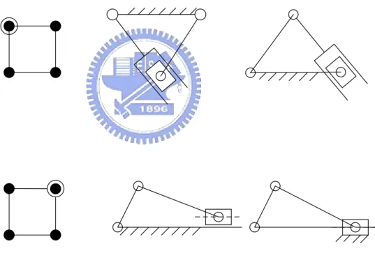
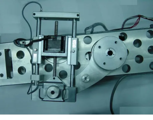
Figure 21 presents kinematic inversions associated with various selections the of ground link of the RRRP kinematic chain [32]. Both the swinging block and the turning block are much less well-known than the slider-and-crank from the same RRRP family, since the output cylinder must swing, which raises manufacturing difficulties. However, current technological advances of the linear motor and the helical motor have greatly simplified the swinging cylinder, such as in the sensor pedestal design, shown in Fig.22.
The typical design of such a rotational control member may involve a gear head with the servomotor, which suffers from excessive weight and backlash problems. The alternative design adopts a direct-drive motor, which however, requires a higher electric power than specified. There the design of the turning block mechanism is well conceived since it exhibits a low weight-to-power ratio.
Figure 23 illustrates the kinematic structures of the swinging-block and the turning-block mechanisms. L represents the length of the ground-link. R represents the length of the output-link. The slider-link, depending on the distance traveled by the motor, has a variable length S. With a single D.O.F., either the swinging block or the turning block mechanism is driven by the input variable S.
The simple trigonometric relation determines the input variable S 22
as a function of the internal angles
θ
andφ
as follows.φ
θ
sin sin ⋅ = L S (3.1) S⋅cosφ
+L⋅cosθ
= R (3.2)The cosine law yields,
S2 =R2 +L2 −2RL⋅cos
θ
(3.3)The internal angle
φ
is known as the transmission angle of theswinging block or the turning block mechanism. In Fig.23, Fi
represents the input force, exerted from the linear actuator. TK represents the output torque transmitted to the output link, and is a function of the transmission angle, as follows.
TK = Fo ⋅R
= Fi ⋅sinφ⋅R (3.4)
The mechanical advantage is maximum only when
φ
= 90± o,discouraging the use of swinging block or turning block mechanism to
beyond its positions of singularity,
φ
= 180o.3.3 Maximum Average Mechanical Advantage
In practice, the swing angle of the output link is specified in the design of the swinging block or turning block mechanism; that is, on
the range of
θ
is specified. A set of dimensions of the swinging blockor the turning block mechanism must be determined to optimize the
mechanical advantage over the specified range ±
ε
, about themiddle-angle
θ
ο of the swing angleθ
, as shown in Fig. 24. Itsapplication must be limited to
ε
< 90o to avoid the singularity. Forexample, the turning block mechanism may be required to function 23
over a range of swing angle of
ε
= 25o, a typical value for radar applications. Nevertheless, the workspace of the swinging block mechanism must also be considered.According to Eqs. (3.1) and (3.2), the transmission angle
φ
relatesto the swing angle
θ
as follows.) cos sin ( tan 1
θ
θ
φ
⋅ − ⋅ = − L R L (3.5)The average mechanical-advantage E could be expressed as the
integral form of the torque with respect to the swing angle
θ
, over aspecified range
ε
with respect to the designing parameter, themiddle angle
θ
± o, as follows. =∫
θθ−+εεθ
ε
o o Td E 2 1 =∫
θθ −+εε ⋅ ⋅φ
θ
ε
o o Fi R sin d 2 1 (3.6)Substituting Eq. (3.5) into the above equation yields,
θ ε ε θ
θ
ε
+ − − + ⋅ = o o RL L R F E i [ 2 cos ] 2 2 2 (3.7)The maximum average mechanical-advantage with respect to the
design parameter
θ
o is obtained by finding the stationary value of theaverage output torque E, as follows.
sin( ) sin( ) 0 2 max min ⎭⎬ = ⎫ ⎩ ⎨ ⎧ − − + ⋅ ⋅ = S S R L F d dE i o o o
ε
θ
ε
θ
ε
θ
(3.8) where, 2 2 2 cos( ) max = R +L − RL⋅θ
o +ε
S (3.9a) 2 2 2 cos( ) min = R +L − RL⋅θ
o −ε
S (3.9b)According to Eq. (3.3), Smin and Smax are actually the minimum
and maximum length extended by the linear actuator, respectively.
In general cases, over a finite swing range
ε
, the input force Fi,the ground link length L, and the output link length R, must all be non-zero, (8), yielding,
(cos
θ
− cosε
)(cosθ
− cosε
)=0R L L R o o (3.10)
The optimal solution for
θ
o is obtained, yielding the maximumaverage mechanical-advantage as,
cos
θ
cosε
L R o = (3.11a) or, cosθ
cosε
R L o = (3.11b)The second derivative of Eq. (3.7), which equals the first derivative of Eq. (3.10) multiplied by a constant k, may be written as,
o o H k d E d
θ
θ
2 sin 2 ⋅ ⋅ = (3.12) where, 0 2 ⋅ ⋅ > = F L R k iε
and, 8 cos 4 cos (1 ( )2) L R L R H = ⋅ ⋅θ
o − ⋅ε
+ (3.13)The middle-angle
θ
o is selected to be positive, as shown in Fig.24; such that sin
θ
o > 0. Hence the sign of Eq. (3.12) depends on thesign of H(
θ
o). For a design free of any singularity,ε
< 90o, that is cosε
> 0, is required. Substituting Eq. (3.11a) into Eq. (3.13), yields, 4 ( )2 1⎟⋅cosε
⎠ ⎞ ⎜ ⎝ ⎛ − = L R H (3.14a)However, substituting Eq. (3.11b) into Eq. (3.13), yields,
4 1 ( )2 ⋅cos
ε
⎟ ⎠ ⎞ ⎜ ⎝ ⎛ − = L R H (3.14b)The maximum value is obtained from either Eq. (3.11a) or Eq. (3.11b) by setting H < 0, which parameter depends on the R/L ratio of the design. That is, the result of Eq. (3.11a) for L > R and that of Eq. (3.11b) for R > L are used to obtain the maximum value.
3.4 Optimal Design
Assuming no energy loss due to friction in the joints or any other viscous damping, the energy output to the output link equals the energy input from the linear actuator, since the total energy is conserved. That is,
∫
=∫
θθo−+εε θ (3.15) o max min TKd ds F S S iwhere Smin and Smax are defined in Eqs. (3.9a) and (3.9b),
respectively. Given a constant input Fi, Eq. (3.15) may be
reformulated as follows.
E Fi D
ε
2= (3.16)
where D denotes the required travel span of the linear actuator, D =Smax − Smin
E is the average mechanical advantage, which was previously
defined in Eq. (3.6). Equation (3.16) shows that the average mechanical advantage E is proportional to the distance traveled by the
linear actuator D. Therefore, a linear actuator that can be extended farther is always preferred for its greater mechanical advantage.
According to Eq. (3.1), the transmission angles
φ
min andφ
max aredefined as follows. max min ) sin( sin S L
θ
oε
φ
= ⋅ + (3.17a) min max ) sin( sin S Lθ
oε
φ
= ⋅ − (3.17b)Where
θ
o fulfills one of Eqs (3.11a) and (3.11b) to yield themaximum average mechanical advantage. According to Eqs. (3.8), (3.17a) and (3.17b),
sinφmin =sinφmax (3.18)
Thus, the travel span of the linear actuator D can be related to the link length L, as follows.
{
sin(θ
ε
) sin(θ
ε
)η
⋅ + − −= L o o
D
}
(3.19)where
η
represents the minimum mechanical advantage and,R F K T sinφ η i min = ⋅ =
The design problem concerns five design parameters, D, L, R,
η
and
ε
. These five design parameters uniquely determine the fourturning block mechanism link lengths and one the middle swing-angle.
Of the five design parameters, the swing angle span
ε
is provided as adesign specification. This set of design parameters can again by normalizing the link length. Consequently, only three normalized
design parameters are to be determined; they are
η
, D/R and L/R.Optimal design problems may be separated into two categories. 27
The first is for L R. Equation (3.11a) is applied to find the
optimal solution. Manipulating and simplifying Eqs. (3.17a), (3.11a) and (3.9a) yield,
≥
η
=cosε
(3.20)For L R, the design parameters
η
andε
are not independent.In design procedure,
η
can not be freely specified for a given swingspan
ε
. Substituting Eq. (3.11a) into Eq. (3.19) and combining withequation (3.20) yields, ≥ =2⋅sin
ε
R D (3.21)The second category of problem has L < R. Equation (11b) is applied to find the optimal solution. Manipulating and simplifying Eqs. (3.17b), (3.11b) and (3.9b) yields,
for R⋅sinθ0 > L⋅sinε :
η
= ⋅cosε
R L
(3.22a)
for R⋅sinθ0 < L⋅sinε :
η
=− ⋅cosε
R L
(3.22b) Since Eq. (3.22a) (3.22b) contradicts the condition that L < R, no
optimal solution exists. The second category is discarded because of the need to obtain a good mechanical advantage.
3.5 Design Procedure:
The design procedure is summarized as follows.
Step 1: Specify
ε
.Step 2: Set the L/R ratio to no less than 1.
Step 3: Obtain
η
and the D/R ratio from Eqs. (3.20) and(3.21), respectively.
For the configuration illustrated in Fig. 25, R = 1, L = 2 and
ε
= 30o are set. The optimal value of the design parameterθ
ο is
obtained from Eq. (3.11a), yielding
θ
ο = 64.34o and D/R = 1. Figure 26presents more general cases subjected to different
ε
versus D/R andε
versusη
. Figure 27 plots the curved surface ofε
and R/L versusθ
ο.Chapter 4 Robotic Safeguard System and Workspace
Analysis
4.1 Reviews
The conventional robotic safeguard systems have been developed from the mechanical hardware safeguard systems to the systems involving electrical hardware devices (such as emergency stop switch, dead-man switch, limit switch, etc.), and the safeguard systems inside and outside the robot working areas. The existing sensor warning systems for the robotic safeguard can be divided into the follows [39]: warning sign system, safety barrier device, pressure pad, inferred, capacitor, microwave, ultrasound, magnetic field, video image, etc. Sensors as defined in this context as the devices that detect if there anyone exists, based on the physical features. These methods have been used for a long time, and work well, however the robot application becomes wider, the conventional sensors warning method show its insufficiency of flexibility and impotence. The robot static positioning problem can be solved via the forward and backward kinematics [40], therefore the robotic movement can be displayed as the animation, and the collision detection can be performed by the computers.
Three levels [41, 42] of the robotic safety envelopes are defined. Level 1 is the maximum envelope, Level 2 is the restricted envelope, and Level 3 is the operating envelope. The robot’s virtual boundary is defined as the Level 3 area, which is dynamically varied with the
operating conditions of the manipulator. The active robotic safeguard system involves not only the static protection areas (Level 1 and Level 2), but also the dynamic area (Level 3). The robot language is implemented for the robot movements, which involve the three levels of the robotic safety commands.
The International Standards Organization (ISO) introduced the Open Systems Interconnection (OSI) Reference Mode [43], the layered network architecture, with the goal of international standardizing protocols governing the networking communication. However Transmission Control Protocol/Internet Protocol (TCP/IP) [44, 45, and 46] doesn’t directly follow the OSI model. Although each network model has the goal of facilitating communication among different types and models of computers, and operating systems, the implementations of each network model present a variety of aspects. Whereas the OSI model was driven by a large standards organization, it took a long time to formulate a draft and adopt it as a standard. In a different situation, TCP/IP was driven by the immediate need of the United States government. The development of TCP/IP isn’t burdened with the same stringent requirements as OSI. Local Area Network (LAN) [47] is a data communication network, typically a packet communication network, limited in geographic scope. A local-area network generally provides high-bandwidth communication over inexpensive transmission media. A local-area network is composed of hardware elements and software elements. Hardware elements belong to three basic categories: a transmission medium, a mechanism for control of transmission over the medium, and an interface between the network and devices that are connected to the network. The software
elements are the sets of protocols, implemented in the devices connected to the network, that control the transmission of information from one device to another via the hardware elements of the network. These protocols function at various levels from data-link layer protocols to application layer protocols. Also, LANs are characterized by a large and often variable number of devices requiring interconnection. LANs have a high bandwidth channel with short propagation delays, however shared by many independent users. A Web server [48] does a great deal of work in making Web pages and sites available to browsers. They are the linking mechanism between you and the Web, between people and pages. Web servers consist of special hardware and software that make it possible to carry out browser request. In this thesis, the client-server architecture is defined as the basis for communication between two robotic programs called the client and the server. A server is any application that provides a service to a network user. A client is any program that makes a request to a server. In general, a client and a server run on different computers. Client-server architecture contrasts with the classical centralized architecture popularized by typical mainframe installations. In a centralized environment, the “clients” are little more than dumb terminals that act as simple data entry / display devices. There’s a minimum of work done at the terminal. The user typically fills in the fields of a form before sending the field data to the central computer. All processing and screen formatting are done on the central computer, and dumb terminal simply displays the preformatted data. In a client-server environment, the client has much greater ability and more freedom with the final visual presentation of the data to the user.
Instead of the data being preformatted to match the way it will be viewed, they are transferred in its “raw” format to the application running on the client computer, which “decides” itself how to display that data. Thus, the “front end” that the user sees can be customized while the “back end” remains unchanged. The Centralized Monitoring and Control Computer is the “client” and the individual robot is the “server”. Any program can be opened to handle several connections simultaneously, to play both client and server at the same time.
4.2 The Active Multi-Robotic Safeguard System
Architecture
The traditional safeguard system is integrated with sensors, and then installed into the hazard areas statically. However, with the application of the robot increases, the traditional safeguard system shows its insufficiency of flexibility and efficiency. The intelligent safeguard system is generated, with some kinds of the high accuracy and performance devices integrated, and the software can be controlled for setting up the hazard areas dynamically, with the different operation types and locations of the robot. The omni-direction magnetic position trackers are integrated with the robots and the operator, with the client-server based networking system, software and hardware integrated, the complete real time data of the multi-robot kinematics and operator movement can be obtained, as shown in Figure 28.
The 3D space objects can be represented in the coordinate relative to the absolute coordinate system, and their position and orientation is in terms of the 4 by 4 homogeneous transformation
matrix which combines both rotation and translation process in a single matrix. During the time t, the point Loc in object A relative to the absolute coordinate can be represented as
) A ( 0 A (0)(t) T (t)Loc Loc = → (4.1)
For calculating the collision detection between object A and object B, the point Loc on object A relative to the local coordinate of the local coordinate can be represented as
) 0 ( 0 B (B)(t) T (t)Loc Loc = → (4.2)
Substitute equation (4.1) into (4.2), then
[
]
(0) A B 1 0 A ) B ( (t) T (t) T (t)Loc Loc = → − → (4.3)Assume the end point Loc is inside the range of object B, then the object A and object B are in the collision condition.
As the depicted previously, the hazard areas determination for the intelligent safeguard system may vary from the robot operational conditions. In order to fortify the safeguard, the hazard areas may be enlarged. Figure 29 shows the coordinate system for the robotic collision detection. Object A refers to the operator, other people, or the robot’s manipulator “wearing” the positioning sensor, and object B represents the main robotic system with positioning sensor also. Referring to this figure, the robot movement will be in slower speed when any objects are falling inside the safety envelope Level 2 (hazard zone), and the robot will be fully stopped when any objects are inside the safety envelope Level 3. The safety envelope Level 3 is defined as the robot’s virtual boundary in this thesis.
With the 3D monitoring display implemented, the robot false movement can be detected, then the three-level robotic safeguard system is functional, and the robot speed is slowed down, or the brake
system works with the control system, to attain the emergency stop function. The real time robotic collision avoidance function can be used as the safeguard system eventually.
4.3 The Robot System Installation and the Kinematics
Analysis
The robot systems have been installed with various safety-sensing devices for the complete safeguard system test. There are two kinds of robot systems used in this research. First, the U-type robot is a non-Cartesian coordinate kinematics mechanism, as shown in Figure 30. This type of the robot is widely used for the industrial field. The U-type robot mechanism entity has a three- D.O.F. manipulator with a two- D.O.F. robot wrist. This open-chain robot system is easy to be assembled, and is convenient for performing its manipulator control in the laboratory. The other type of the robot system, as shown in Figure 31, is the parallel-linked robotic system designed for the laboratory used, in order to verify the system theory. The kind of robot platform belongs to the six- D.O.F. Cartesian coordinate kinematics mechanism system, with feedback, high compliance and stability.
For obtaining the robot motion in the space, the kinematics is a very common problem to discuss the relation between robot joint space and Cartesian space. The kinematics analysis for the robot system is significant in this thesis, to integrate the robot virtual reality real time display with the real robot mechanism precisely. For instance, if we choose the U-type robot system as case of the motion mechanism for the robotic safeguard, its forward kinematics can be
described as follows: (4.4) ⎥ ⎥ ⎥ ⎥ ⎦ ⎤ ⎢ ⎢ ⎢ ⎢ ⎣ ⎡ = 1 0 0 0 p r r r p r r r p r r r T z 33 32 31 y 23 22 21 x 13 12 11 base ker trac where
(
2 3)
1 11 =cosθ cos θ +θ r(
2 3)
1 21 = sinθ cos θ +θ r(
2 3)
31 = sin− θ +θ r 1 12 = sin− θ r 1 22 = cosθ r 0 32 = r(
2 3)
1 13 =cosθ sin θ +θ r(
2 3)
1 23 =sinθ sin θ +θ r(
2 3)
33 = cos θ +θ r(
)
⎟ ⎠ ⎞ ⎜ ⎝ ⎛ θ + θ +θ θ = 2 3 arm lower 2 arm upper 1 L cos L cos cos x p(
)
⎟ ⎠ ⎞ ⎜ ⎝ ⎛ θ + θ +θ θ = 2 3 arm lower 2 arm upper 1 y sin L c L cos p os(
2 3)
arm lower 2 arm upper z L L s p =− sinθ − in θ +θIts inverse kinematics can be limited into a three D.O.F. mechanism, and if the input is position, then:
) p , p ( tan a − y x = θ1 2 ⎟ ⎟ ⎠ ⎞ ⎜ ⎜ ⎝ ⎛ − − + ⎟⎟ ⎠ ⎞ ⎜⎜ ⎝ ⎛ θ = θ − 2 2 2 2 1 1 3 arm lower arm upper z x p L L cos p cos 36
⎟ ⎠ ⎞ ⎜ ⎝ ⎛ + θ − θ − = θ − 3 3 1
2 cos p atan2 L L cos L sin
arm lower arm lower arm upper z (4.5)
If the arm lengths, robot end effector movements are known, then the robot joint rotation angles can be derived from equation (4.5). Therefore, the robot central monitoring system can use of the robot kinematics to implement the 3D real time display, trackball control, position tracker control, and other sensor’s control functions, interactively. The kinematics calculation for a parallel robot mechanism is in a similar way.
4.4 The Robotic Operation and Control Interface
Program
The robotic operation and control interface program is written in C++ for Windows. This program contains four control panels: graphic display control, robot multi-axis control buttons, controllable parameter settings, and control status display. The position tracker driver program is added into this program, in order to process the tracker data for the robot upper arm. The interface program for the industrial robot is shown in Figure 32.
The Graphic Display Control window shows the robotic motion. With the command for each axis, the direct kinematics calculation, and the related graphics calculation, the accurate 3D robotic motion display can be obtained. The controller is in the “wait state” for the control system, and the high-level commands are issued from the client (Windows NT) VR control panel, and the motion program is sent out from the fiber network to control the server - the robot. Figure 33 shows the networking for the industrial robot controller interface.