碼同步之相量獲取方法

國立交通大學

電信工程研究所

碩士論文

碼同步之相量獲取方法

A Phasor Domain Acquisition Method

for Code Synchronization

研究生：林群明 Student: Chiun-Ming Lin

指導教授：高銘盛 博士 Advisor: Dr. Ming-Seng Kao

碼同步之相量獲取方法

A Phasor Domain Acquisition Method for Code

Synchronization

研究生：林群明 Student: Chiun-Ming Lin

指導教授：高銘盛 博士 Advisor: Dr. Ming-Seng Kao

國立交通大學

電信工程研究所

碩士論文

A Thesis

Submitted to Institute of Communication Engineering College of Electrical Engineerinring and Computer Engineering

National Chiao Tung University In partial Fulfillment of the Requirements

For the Degree of Master of Science

In

Communication Engineering

July 2012

Hsinchu, Taiwan, Republic of China

碼同步之相量獲取方法

學生：林群明 指導教授：高銘盛 博士

國立交通大學

電信工程研究所

摘要

「碼同步」在展頻通訊系統中是一項重要且值得探討的議題，而傳統的作法是在時域 上做序列比對。 藉著快速傅立葉轉換(FFT)，我們可以將碼序列轉變為相量，接著利 用逆傅立葉轉換(IFFT)，即可找到輸入序列和本地序列的相位差。當碼序列長度增加 時，所耗費的運算量也隨之增加。 本論文中，我們提出一個新的「碼同步」方法，它不需作逆傅立葉轉換以減少運算 量。這個方法主要利用複數相量之間的相位關係，藉此可以擷取所需的相位差。在分 析複數相量的統計特性之後，我們提出一個簡單的方法求相位差。接著， 我們進一步 提出一個進階的方法以提升系統的準確度。最後，我們利用電腦模擬驗證所提的理論， 其中分析的重點在於相位變異數的變化以及估測的準確度。模擬的結果顯示，所提方 法可減少許多運算量並在高 SNR 的環境下可以獲致良好的結果。

A Phasor Domain Acquisition Method for

Code Synchronization

Student: Chiun-Ming Lin Advisor: Dr. Ming-Seng Kao

Institute of Communication Engineering

National Chiao Tung University

Abstract

Code synchronization is a critical issue in spread spectrum communication systems. The traditional method to achieve code synchronization is via serial search in the time domain. By performing Fast-Fourier-Transform (FFT), the code sequence can be projected to the phasor domain. Then, code phase between local sequence and input sequence can be found via Inverse-Fast-Fourier Transform (IFFT). However, as the code length increases, the computation increases considerably.

In this thesis, we propose a new method for code synchronization in the phasor domain without IFFT. The method is based on the phase relationship of complex phasors, whereby we can extract code phase via phasor phases. We analyze the statistical property of complex phasors and design a simple method to extract the code phase. Moreover, we further design an improved method to enhance the accuracy under noisy condition. Computer simulation is performed to verify the proposed scheme, which focuses on variance reduction and estimation accuracy. It can be demonstrated that the proposed method works well without much computation while acceptable accuracy is achievable in high SNR environment.

誌 謝

在本論文中，首先我最感謝的是我的指導教授，高銘盛 博士。不論在課業或是研 究，甚至是人生規劃方面，他總是在旁指導著我。並且老師的指導相當細心且有耐心， 不論是多小的問題他都能很有條理的教導我們。因此，老師就像父親也像朋友。從老 師身上可以學習到許多做人處事的態度及方法，包括老師的好教養以及做事謹慎的態 度。相信這是能從老師身上學到且受用一生的好習慣。 另外，感謝所有實驗室的同學及學長姐們。有問題能一起討論真的很好，使我在 求學方面減少許多困難。也非常感謝我的家人，能給予我優良的求學佳境，在讓我全 心全意的攻讀碩士學位。感謝我的姊姊，因為他非常疼我這個弟弟。也感謝我的姊夫-陳建銘 大夫，希望他能好好對待我姊。最後，特別感謝一個重要的人-「洗濾鏡」小 姐。他在我的研究所生涯中，給予我一個良好的管道宣洩我的情緒，激發我的潛能。 感謝她，希望人生會因此而更美好。 謹將此論文獻給所有幫助過我的人們，共勉之。 2012/07/09

Contents

中文摘要

i

English Abstract

ii

誌謝

iii

Contents

iv

List of Figures

vi

Chapter 1 Introduction

1

Chapter 2 Properties of Phasors

4

I. Noiseless Condition……….……...4

II. Noisy Condition………...7

A. Signal Model………..7

B. Vector Analysis………11

Chapter 3 The Proposed Method

14

I. Noiseless Condiotn...14

III. A Simple Phase Estimation Method………..17

IV. An Improved Method………..19

V. New Local Sequence………...25

Chapter 4 Simulation Results

28

I. First Estimation...28

II. Second Estimation...30

III. Third Estimation...33

IV. Recursive Algorithm...36

Chapter 5 Conclusions

40

List of Figures

Figure 1.1: The traditional communication system………3

Figure 2.1: The vector concept of W ………..11 i

Figure 3.1: The estimation flow chart………24

Figure 3.2: A new local sequence ZL………...25

Figure 3.3: The vectors concept of P and i G ………...27 i

Figure 4.1: The flow chart in simulation………...28

Figure 4.2: The standard deviation of _i in terms of SNR………...29

Figure 4.3: The standard deviation of q1………30

Figure 4.4: The standard deviation of _i and ' under different SNR conditions……...31

Figure 4.5: The standard deviation of q2………33

Figure 4.6: The standard deviations of _i and _i………..34

Figure 4.7: The standard deviations of  ' and

1

'

k



………...35

Figure 4.8: The standard deviation of q3………...36

Figure 4.9: The standard deviation of  ' and

2

'

k



Figure 4.10: The standard deviation of 1 ' k  and 2 ' k  ………..……. 38

Chapter 1

Introduction

I. Overview

In the traditional digital communication system as shown in Fig-1.1, the information source generates particular symbols at a specific rate. The source encoder translates these symbols into sequences of 0's and 1's. Next, the channel encoder further translates the obtained sequences into another sequences of 0's and 1's, so as to realize high transmission reliability and efficiency. Following the channel encoder, the modulator accepts the encoded bit stream and converts them to signal waveforms suitable for transmission. After passing through the channel, the waveform suffers from amplitude/phase distortion due to the noise, transmission delay and multipath effect. Therefore, the waveform we get at the receiving end might not be the same as the transmitting one. So the primary objective of a communication system is to suppress the bad effects coming from the channel as much as possible.

The inverse process takes place at the destination side. The demodulator converts the signal waveforms to sequences of 0's and 1's, and then the channel decoder translates this sequence to the original one. It also performs error correction and clock recovery. The source decoder finally translates the sequence of into original signals. Recovering the information sequence from the distorted waveform is the main purpose of a communication receiver.

Synchronization in telecommunications networks is the process of aligning the time scales of transmission and switching equipment so equipment operations occur at the correct time and in the correct order. Synchronization requires the receiver clock to acquire and track the periodic timing information in a transmitted signal. The transmitted signal consists of data that is clocked out at a rate determined by the transmitter clock. Signal transitions between 0’s and 1’s contain the clocking information and detecting these transitions allows the clock to be recovered at the receiver.

II. Our work

Our work will not focus on how to recover the information sequence from the distorted waveform, instead the main objective we are interested in is the “code synchronization”, i.e. to find the code phase shift between the incoming sequence and the local sequence at the receiver. This issue is critical in spread spectrum systems where code synchronization must be achieved before signal demodulation.

In order to simplify the problem, we consider the noiseless condition first. When there is no noise accompany with the input sequence, some phase delay exists between the input sequence and the local one. We denote q as the particular shift between them. If the accurate value of q is got, the synchronization is completed. Assume SI (x0,x1,....,xN1) is the input sequence and S_L (y₀,y₁,...,y_N1) is the local sequence, wherey_k x_kq and N is the code length. Our goal is to find the code-phase shift between S and _I S , i.e. the value _L

of q. We’ll introduce the classic way on dealing with this problem, i.e. the Fast Fourier Transform (FFT) method. By transforming the sequences to the frequency domain via FFT, we find that “q” is imbedded in the phases of complex phasors. Thus we can get it accurately by performing Inverse Fast Fourier Transform (IFFT). In general, N is a large number so that the computation of FFT and IFFT grows rapidly when N increases. To reduce the computation

load, we propose a new scheme which can accurately estimate “q” without IFFT.

The main idea is a little bit tricky. Because the information of q is embedded in the phase of each phasor in frequency domain, we can estimate the code phase via inner product of different phasors. However, even though in high SNR condition, we can’t be sure if the observed phase is close enough to the correct one because of the disturbance coming from noise. The intuitive solution is to reduce the noise variance to some extent such that the estimated code phase will have little probability to be erroneous. Therefore, we design a simple but effective method to decrease the noise variance. It can be proved that the proposed scheme can reduce the computation without losing much accuracy.

The thesis is organized as follows. In Chapter 2, we will introduce the phasor concept of FFT and analyze its properties. Next, the details of the proposed system will be described in Chapter 3 and simulation results will be demonstrated in Chapter 4. Finally, we present the conclusions of this study in Chapter 5.

Chapter 2

Properties of Phasors

Suppose that S is the input sequence and _I S is the local sequence, given as _L

0 1 1

( , ,...., )

I N

S  x x x _ and S_L (y₀,y₁,...,y_N1), wherex_i,y_i (1,1). We assume q phase shift between these two sequences, i.e.y_k x_kq.

I. Noiseless condition

In the beginning, we consider the noiseless condition which is easy to be analyzed. For the two sequences of interest, when FFT is performed we get

jNik k N k i x e X  2 1 0   



 ,i0,1,2,...,N1 (2.1) jNik k N k i y e Y  2 1 0   



 ,i0,1,2,...,N1 (2.2) Let | | ji i i X  X e (2.3) | | j i i i Y Y e (2.4)

where i and i denote the phases of X and i Y , respectively. i

iq N j i iq N j q k i N j q k N k ik N j q k N k ik N j k N k i e X e e x e x e y Y      2 2 ) ( 2 1 0 2 1 0 2 1 0                  







(2.5)

Note that X and _i Y share the same amplitude but differ by_i 2 iq N



in their phases, where

N i0,1,2,..., . Thus we have |Xi||Yi| (2.6) _{i i} 2 iq N     (2.7) Next, we define * i i i V  X Y = 2 2 | | jNiq i X e    (2.8) Assume S and _I S are maximum-length sequences (m-sequences), it can be proved that _L

0 1 0 1 | | | |       i if N i if Y X_{i i} (2.9) Using (2.9) we get

0 , ) 1 ( 0 1 2       i if e N i if V iq N j i  (2.10)

From (2.10) we know that the code phase “q” is embedded in the phase of V . Note that _i V ₀

contains no information about q , which is ignored in the following analysis.

Using (2.10), we can get the value of q via IFFT. Letv denote the IFFT of _k V , given as _i

follows: jNik i N i k Ve v  2 1 0



   , k=0,1,2…..,N-1 (2.11) When k q, we get 2 2 1 0 2 2 2 1 0 2 1 0 ) 1 )( 1 ( 1 | | | | N N N X e e X e V v i N i iq N j iq N j i N i iq N j i N i q         







          (2.12) When k q, we get

N N e N e X X e X e e X e V v k q i N j N i k q i N j i N i k q i N j i N i ik N j iq N j i N i ik N j i N i k                              











) 1 )( 1 ( 1 ) 1 ( 1 | | | | | | | | ) ( 2 1 1 ) ( 2 2 1 1 2 0 ) ( 2 2 1 0 2 2 2 1 0 2 1 0       (2.13)

Therefore, by looking for the maximum among{v , the correct code phase can be got. k}

II. Noisy condition

A. Signal model

Under noisy condition, a gaussion noise denoted as k is added to the transmitted sequence.

In this case, the input sequence becomesS_I (w₀,....,w_N1) and w is given by _k

w_k s g n (x_k _k) (2.14)

where “sgn()” denotes the sign function, i.e.sgn(z)1 if z0,sgn(z)1, if z0. To ease the analysis, we modelw as k

wk xkkxk (2.15)

w_k  x_k (2.16)

which means error occurs due to_k. When_k 0, we have

w_k  x_k (2.17)

which means no error occurs.

Let P denote the chip error probability. From (2.15), it is easy to have the following _e

probabilities:

e

k P

P( 2) (2.18)

P(_k 0)1P_e (2.19)

Thus, ifP is known, the statistical property of_e w can be derived. _k

For the input sequence(w0,w1,...,wN1), we perform FFT to get

ik N j k N k i we W  2 1 0   



 , i0,1,....,N1 (2.20)

2 1 0 2 1 0 2 2 1 1 0 0 2 1 0 2 1 0 [ ] [ ] [ ( ) ] [ ] [ ] [ ] N _{j ik} N i k k N _{j ik} N k k k k N _{j ik} N _{j ik} N N k k k k k N _{j ik} N i k k k N _{j ik} N i k k k E W E w e E x x e E x e x e E X x e X E x e            _   _   _  _    _   _          













(2.21) Since E[k]2Pe0(1Pe)2Pe (2.22) Thus i e i e i ik N j k N k e i i X P X P X e x P X W E ) 2 1 ( ) )( 2 ( ) 2 ( ] [ 2 1 0           



 (2.23)

Let A denote the mean of _i W , then _i

i e

i P X

A (12 ) (2.24)

UsingA , we can model _i W as _i

where n is a zero-mean complex random variable. _i

The variance of n , denoted as _i _n2, can be derived as follows:

2 * * * * * * * 2 | | ] [ ] [ ] ) )( [( ] [ i i i i i i i i i i i i i i i i i n A W W E A A W A W A W W E A W A W E n n E            (2.26)

It can be proved that

E[W_iW_i*]|X_i|2 4P_e|X_i|2 4P_eN (2.27) Thus 2 2 2 2 2 2 2 | | 4 4 | | ) 2 1 ( 4 | | 4 | | i e e i e e i e i n X P N P X P N P X P X         (2.28) From (2.9) , we get _n2 4P_eN4P_e2(N1)4P_e(1P_e)N (2.29) When N is large, we can model n as a zero-mean gaussian random variable whose _i

B.. Vector analysis

Now, we would like to apply the concept of vector to help analysis. Let

j i i

i W e

W | |  (2.30) where _i is the phase of W . As shown in Fig. 2.1, if we look _i W ,_i A and _i n as vectors in _i

the complex plane, from (2.25) the following relationship holds:

Wi Ai ni      (2.31) Im n i W i _i A _i _i Re Fig. 2.1: The vector concept of W i

In Fig. 2.1, we have

_i _i _i (2.32)

angle between W_i and A_i. Note that _i is a random phase caused by noise. Let * ( ) 2 | || | | || | i i i i i i j i i j iq N i i V W Y W Y e W Y e   _          (2.33)

Obviously, the phase of V still contains the information of_i q, but is disturbed by_i. When IFFT is performed, we obtain:

jNik i N i k Ve v  2 1 0



   , k 0,1,...,N1 (2.34) If k q, then iq N j j i i N i iq N j j i i N i iq N j i N i q e e Y W e e Y W e V v i i i i i        2 ) ( 1 0 2 ) ( 1 0 2 1 0 | || | | || |               







(2.35) From (2.7) we get _{i i} 2 iq N      (2.36) Hence

) s i n | | c o s | | ( 1 | | 1 | || | 1 0 1 0 1 0 1 0 i i N i i i N i j i N i j i i N i q W j W N e W N e Y W v i i    









                (2.37)

Owing to the symmetric property of FFT, the imaginary part of v_q is zero so that

i i N i q N W v 1 | |c o s 1 0



     (2.38)

Note that for a given W , because i i is a random variable so that |Wi|cosi is random

Chapter 3

The Proposed Method

Since the computation of FFT and IFFT is proportional toNlogN, it results in considerable computation when N is large. Therefore, we intend to reduce the computation by using the phase information of complex phasors. It is found that the proposed method can much reduce the computation in high SNR condition. The details of our method are described below.

I. Noiseless condition

First, we review the formulas got in the previous chapter under noiseless condition. Assume

0 1 1

( , ,...., )

I N

S  x x x _ is the input sequence and SL (y0,y1,...,yN1) is the local sequence, wherey_k x_kq. When FFT is performed, we get

jNik k N k i x e X  2 1 0   



 ,i0,1,2,...,N1 (3.1) jNik k N k i y e Y  2 1 0   



 ,i0,1,2,...,N1 (3.2) iq N j i i i i e X Y X V  2 2 * | |     ,i0,1,2,...,N1 (3.3)

When i0, it is obvious that the phase of V contains the information about q. Note that _i

2 2 ( 2 ) j iq j iq n N N e e   _     (3.4) for any integer n , there is phase ambiguity in the phase of V . This fact should be carefully _i

considered in estimating q. From (3.3) we get 2 * 2 1 1 1 | 1| j q N V X Y X e      (3.5) Because 0qN1 so that 0 2 q2

N , there is no phase ambiguity presents in the

phase of V . Thus we can obtain q directly from the phase of 1 V under noiseless condition. 1

However, the problem becomes complicated when noise presents.

II. Noisy condition

In noisy condition, the input sequence becomes S_I (w₀,w₁,...,w_N1), where w_k  x_x _k

and k is a gaussian noise. As before, we perform FFT to get

jNik k N k i we W  2 1 0   



 , i0,1,....,N1 (3.6) We can express W as _i j i i i W e W | |  (3.7) where i is the phase of W . Let i

j i i i i i WY V e V  * | |  (3.8)

From (2.34), the phase of V is given as _{i i} iq _i N   _    2 (3.9)

where _i is a random phase caused by noise. Apparently,_icontains the information of q, which can be employed to estimate the code phase.

Under noisy condition, from (3.9) we get

₁ 2 q ₁ N

 _

    (3.10)

where 1 is the random phase caused by noise. Define

) 2 ( ₁ 1     N r o u n d q (3.11)

where “round(z)” denotes the closest integer of z. We may take q as the 11

st

estimation of

q and define

  q1 q q1 (3.12)

where q₁ indicates the error between q1 and q.

It is noteworthy to mention that 2

N

 is a huge number when N is large, which means

the error phase in 1 could possibly be amplified by a large factor in (3.11). In other words,

III. A simple phase estimation method

Using the phases of V given in (3.10), we can get the 11

st

estimation and then obtain q1.

However, the random phase ₁ and a large value of N may result in unacceptable estimation error. This problem can be resolved with the help of other phases of V . _i

The intuitive way to improve the estimation accuracy is to reduce the variance caused by

1

 as much as possible. According to the Law of Large Numbers, the average of random variables obtained from a large number of trials is close to their expected value, and tends to become closer as more trials are performed. It is obvious that the terms Vi (for i>1) can be

used since they do contain the information of q. However, we can’t employ them directly due to the inherent phase ambiguity accompanied with their phases. In order to overcome phase ambiguity, we propose the following approach. Let

0 1 2 ( ) * 0 0 1 | 0| | 1| j q N F V V V V e  _{  }     2 3 2 ( ) * 1 2 3 | 2| | 3| j q N F V V V V e  _{  }     4 5 2 ( ) * 2 4 5 | 4| | 5| j q N F V V V V e  _{  }     ‧ ‧ ‧ 2 1 2 ( ) * 2 / 2 2 1 | 2 | | 1| N N j q N N N N N N F V V V V e  _{ }              (3.13) In general, 2 2 1 2 ( ) * 2 2 1 | 2 | | 2 1| i i j q N i i i i i F V V V V e  _{ }          (3.14)

where each _i in (3.13) is an independent random variable. Eq. (3.14) could be rewritten as ) 2 ( 1 2 2 | | | | j Nq i i i i V V e F   _     (3.15) where_i _2i _2i1. Note that the phase of Fi can be divided into two terms, i.e. the

co-phase term iq N



2

and the random phase term_i.

When the set of {F_i,i0,1,...,N2} is available, we define

i M i F M f



    1 0 1 (3.16)

where M is an integer. We may express f as

j

f  f e (3.17)

where  is the phase of f . When N is sufficiently large, according to the Law of Large

Numbers we get

2 q N



  (3.18) Therefore, could be expressed as

' 2 _    q N (3.19)

than of βi, which will result in more precise estimation of 2 q N  . We will demonstrate it with the simulation to be presented in Chapter 4.

After  is got, we define

) 2 ( 2    N r o u n d q (3.20) where q denotes the 22

nd

estimation of q. Obviously,q will be more accurate than q2 1.

Moreover, the error of the 2nd estimation is given as

q₂ qq₂ (3.21)

IV. The improved method

As shown above, we may apply the Law of Large Numbers to lower the variance in phase estimation. However, the estimation error may not be small enough since it should be less than 2/N in order to get a correct estimate of q. When N is large, as is usually the case, q₂ may not be small enough. Therefore, we are obliged to further reduce the variance by using the special relationship given in (3.8).

In probability theory, ifXis a random variable and a is a constant, we have the

following equality: ( ) 1₂ V a r(X) a a X V a r   (3.22) where “Var(z)” denotes the variance of a ransom variablez. When a1, the variance of

a

After the 2nd estimation, we take  as the estimate of q N



2

, which may deviate from

q N



2

by a random phase '. Assume k is an integer and k 2. If  is close to q N



2

, it

is expected that k is close to 2 kq N



. The idea is: if we can get a good estimate of

2 k

q N



, then a better estimate of q N



2

is got due to the multiplication factor of k. However,

the phase ambiguity problem possibly occurring in the term 2 kq N



should be carefully considered.

Now, we begin to describe the proposed method. Assume k 2 is a given integer. Let

0 2 ( ) * 0 0 | 0| | | k j kq N k k G V V V V e  _{  }     1 1 2 ( ) * 1 1 1 | 1| | 1| k j kq N k k G V V V V e  _{ }          2 2 2 ( ) * 2 2 2 | 2| | 2| k j kq N k k G V V V V e  _{ }          ( 3.23) ‧ ‧ ‧ ( 2 ) / 2 ( 1 ) / 2 2 ( ) * ( 1) / 2 ( 1) / 2 ( 1) / 2 | ( 1) / 2| | ( 1) / 2| N k N j kq N N N k N N k N G V V V V e  _{ }                 In general, 2 ( ) * | | | | j Nq i k i i i k i i k i G VV V V e  _{ }          (3.24)

Note that due to the symmetric property of FFT, we only take i=1~ 1 2

N

in the above equation.

Asαi, i=0,1,2,…, N-1, are independent random variables, the term ( i i k ) could be

expressed as a random variable _i whose variance is the same as _i. Then we obtain

2 ( ) * 1 | | | | , i=1,2,3,..., 2 i j kq N i i k i i i k N G VV V V e  _        (3.25) where _i  _i _{i k} and ) ( ) ( _i Var _i Var    (3.26)

Next, by summing G_i we get

i M i G M g



   1 0 1 (3.27) Assume j g  g e (3.28) where 2 ( k q ') mod 2 N      (3.29)

In (3.29), the variance of ' will be much smaller than of i. Note that because of the

mod-2 operation, in general  is not equal to 2 kq '

N

 _

 . This fact should be taken into account in estimating q.

For a given , from (3.29) we have the following equality:

2 k q ' 2n N

 _{  }

   (3.30)

where n is an unknown integer sinceq is still unknown. Suppose that n is known, then

2n 2 ' q k N k   _  _ (3.31) Let h 2n 2 q ' k N k         (3.32)

We take h as the estimation of 2 q N



, whose mean is given by

_h 2 q E[ ' ] 2q

N k N

  

    (3.33)

whereE[ '] 0 is assumed. On the other hand, the variance of h is given by

2 2 2 2 ' 2 ' [( ) ] [( ) ] 1 h E h h E k k          (3.34)

where _2_' denotes the variance of '. It is easy to see the variance of h can be much reduced if k is large.

It’s noteworthy to mention that in estimating the phase of 2 kq N



k, where q N



2



 . When we multiply  by k, the error phase accompanied with  is also amplified. As a result, although a large k is desired to reduce the variance of h, it also increases the risk of erroneous mod-2 operation. Therefore, choosing an appropriate value of k is a critical issue.

When k is close to 2n , it is probably for erroneous mod-2 operation to occur. Accordingly, we choose k to be around (2n1) to avoid it. Because the larger of k, the more risk of erroneous mod-2 operation, for safety reason in the beginning we take

k  3 (3.35) In turn k is calculated as

k round(3)

 . (3.36)

When k 3 is taken, we get n1 in (3.30). After a more accurate value of 2 q N



is got, we can increase k by taking a larger n so as to further reduce the error phase. Thus,

we may design a recursive algorithm to gradually increase k. The algorithm is shown in Fig. 3.1, whose operation is described below.

Assume q

N



2



 has been obtained. First, we take n1 and get k k₁ with (3.36). After a more accurate estimate of q

N

h2 is got, we set nn1 and get k k₂

to obtain a more accurate estimate of q N



2

. The process can be repeated until the required accuracy is met.

Xi,Yi Recursive Process n=n+1 The nth estimation

Fig 3.1: The estimation flow chart

1 2 1 N j i i

f

F

f e

  









(2 1) n n k round h      _{ }   1 2 1 = N j i i g G g e   



 2n h k    Vi=XiYi* * 1 i i i

F



V V

_ * n i i k i G V V _ i V i F Let h= n k i G 

V. New local sequence

In the above method, when q is small the estimated q N



2



 will be close to zero, in this case k will be a rather large number to make k 3. Under this circumstance, it has high risk for erroneous mod-2 operation. Therefore, we have to design a scheme to resolve this problem.

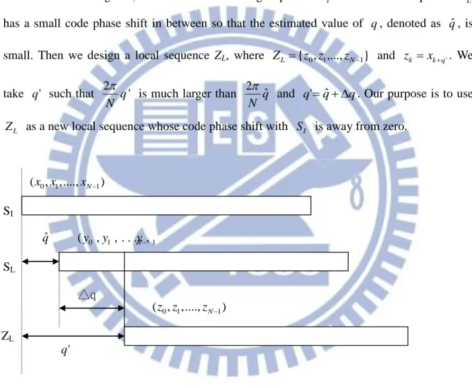
As shown in Fig. 3.2, we assume the incoming sequence S and the local sequence I S L

has a small code phase shift in between so that the estimated value of q, denoted as qˆ, is small. Then we design a local sequence ZL, where ZL {z0,z1,...,zN1} and zk xk q '. We

take q' such that 2 q'

N



is much larger than q N ˆ

2

and q'qˆq. Our purpose is to use

L

Z as a new local sequence whose code phase shift with S is away from zero. I

( , ,....,x x0 1 xN1) SI qˆ (y₀ ,y₁ , . . . . ,_Ny_{ 1} ) SL △q q'

Fig 3.2: A new local sequence ZL.

Under noiseless condition, we have qˆq. When FFT is performed, we get the following equation:

0 1 1

( , ,....,z z z_N) ZL

2 1 0 2 1 ' 0 2 2 1 _{( ') '} ' 0 2 ' N _{j ik} N i k k N _{j ik} N k q k N _{j i k q j iq} N N k q k j iq N i Z z e x e x e e X e       _   _    _{ }        







(3.37) Let U be defined as _i U_i  X Z_i *_i ,i0,1,2,...,N1 (3.38) The relationship between V and _i U is given by _i

* 2 ' 2 2 ( ) 2 2 2 2 2 | | | | | | i i i j iq N i j i q q N i j iq j i q N N i j i q N i U X Z X e X e X e e V e                        (3.39)

It’s obvious that there is 2 i q N

 _

phase difference between Vi and Ui. In (3.25), we have

2 ( ) * 1 | | | | , i=1,2,3,..., 2 i j kq N i i k i i i k N G VV V V e  _        (3.40)

q k N j i q k N j k i i q k i N j k i q i N j i k i i i e G e V V e V e V U U P                     2 2 * ) ( 2 * 2 * (3.41)

As shown in Fig 3.3, the two phasors G and i P have a phase difference of i 2 q

N

 _

in

between. By choosing an appropriate value of q, it is easy to make 2 q'

N



away from zero. Thus, when Z is used as the new local sequence, the same algorithm can be applied to get L

the estimate of q'. After q' is got, it is easy to obtain qq'q, while q is a known parameter which represents the code phase between S and L Z . L

Im Re Fig 3.3: The vectors concept of Pi and Gi

2 q N   2 i q N    i G i P

Chapter 4

Simulation Results

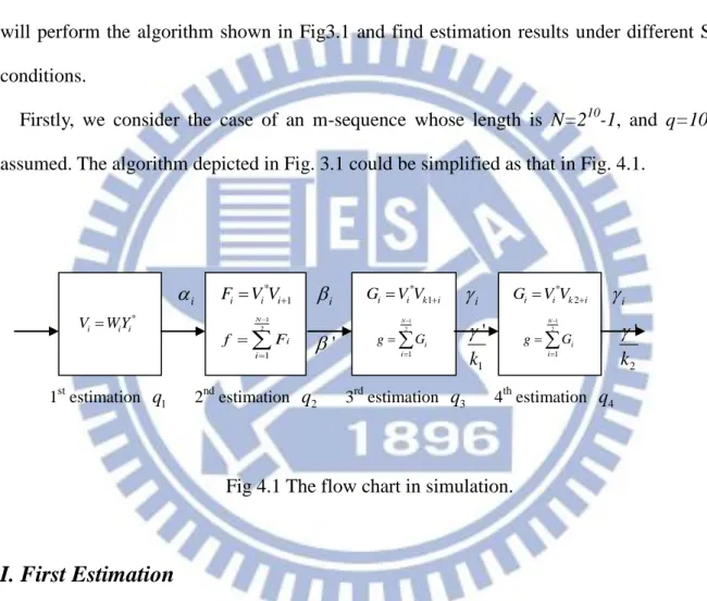
After introducing the proposed algorithm, we will show simulation results in this chapter. We will perform the algorithm shown in Fig3.1 and find estimation results under different SNR conditions.

Firstly, we consider the case of an m-sequence whose length is N=210-1, and q=100 is

assumed. The algorithm depicted in Fig. 3.1 could be simplified as that in Fig. 4.1.

i i i i ' 1 ' k  2 ' k 

1st estimation q₁ 2nd estimation q₂ 3rd estimation q₃ 4th estimation q₄

Fig 4.1 The flow chart in simulation.

I. First Estimation

Recall that in the first step, we employ V which contains information of q without phase 1

ambiguity as the initial guess, and then obtain q1 as the 1st estimation. The equations involved

in this estimation are given as follows:

* 1 1 1 1 | |1 j V W Y V e (4.1) * i i i V WY * 1 i i i F V V_ 1 2 1 N i i f F   



* 1 i i k i G V V  1 2 1 N i i g G    * 2 i i k i G V V _ 1 2 1 N i i g G   

₁ 2 q ₁ N  _     (4.2) ) 2 ( ₁ 1     N r o u n d q (4.3)   q₁ q q₁ (4.4)

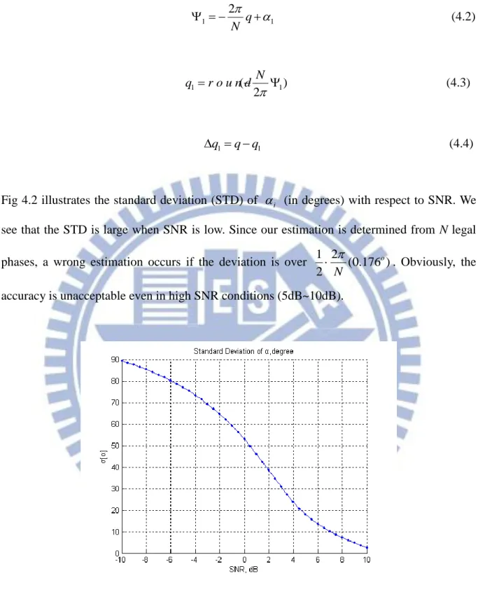
Fig 4.2 illustrates the standard deviation (STD) of _i (in degrees)with respect to SNR. We see that the STD is large when SNR is low. Since our estimation is determined from N legal phases, a wrong estimation occurs if the deviation is over 2 (0.176 )

2

1 o

N



 . Obviously, the

accuracy is unacceptable even in high SNR conditions (5dB~10dB).

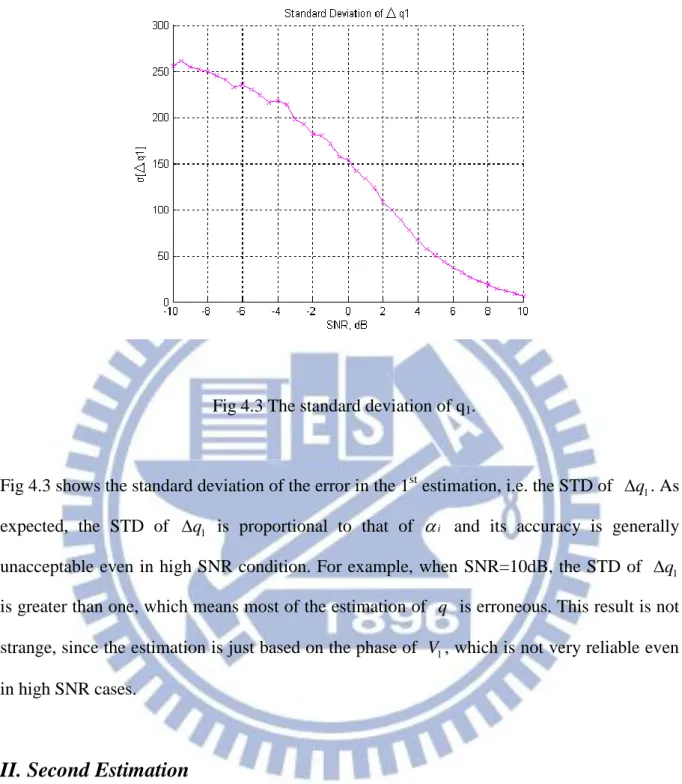
Fig 4.3 The standard deviation of q1.

Fig 4.3 shows the standard deviation of the error in the 1st estimation, i.e. the STD of q₁. As expected, the STD of q1 is proportional to that of i and its accuracy is generally

unacceptable even in high SNR condition. For example, when SNR=10dB, the STD of q₁

is greater than one, which means most of the estimation of q is erroneous. This result is not strange, since the estimation is just based on the phase of V , which is not very reliable even ₁

in high SNR cases.

II. Second Estimation

In the second estimation, we transfer V to be i F which contains the information of q as i

well. Since the random phase of F , denoted as _i _i, is equal to  _i _i1, the variance of _i is larger than of i. However, we may apply the Law of Large Number to lower the variance

by summing phasors. The equations involved in this procedure are shown as follows:

2 ( ) * 1 | | | 1| i j q N i i i i i F VV V V e  _       (4.5)

1 2 ₍2 _') 1 N q j j _N i i f F f e f e  _     



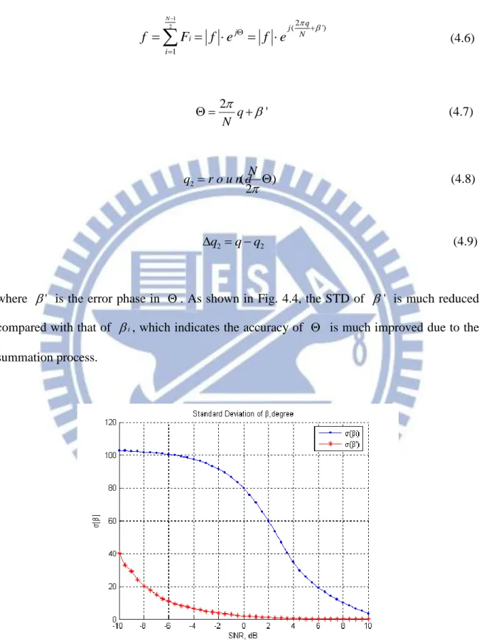
    (4.6) 2 ' q N  _    (4.7) ) 2 ( 2    N r o u n d q (4.8) q2 qq2 (4.9)

where ' is the error phase in . As shown in Fig. 4.4, the STD of ' is much reduced compared with that of i, which indicates the accuracy of  is much improved due to the

summation process.

Fig 4.4 The standard deviation of _i and ' under different SNR conditions.

theory, if X , _i i1,2,...,n, are independent and identically distributed random variables, we have ) ( 1 ) 1 ( 1 i i n i X Var n X n Var



  (4.10) Substituting 1 2 N

for n in (4.1) and take square root in both sides, the relationship

between the STDs of ' and _i are given by

1 ( ' ) ( ) 1 2 1 ( ) 22.616 i i N            (4.11)

Because i and ' are random phases in the complex domain, there are two special

properties of them:

(1) The range of phase is [ , ], (2) j j( 2k )

e e   .

These two properties make the relationship between (') and (i) becomes nonlinear, but not the linear one given in (4.11). However, Eq.(4.11) is still an important reference for our simulation, because it is close to the simulated result when SNR is high.

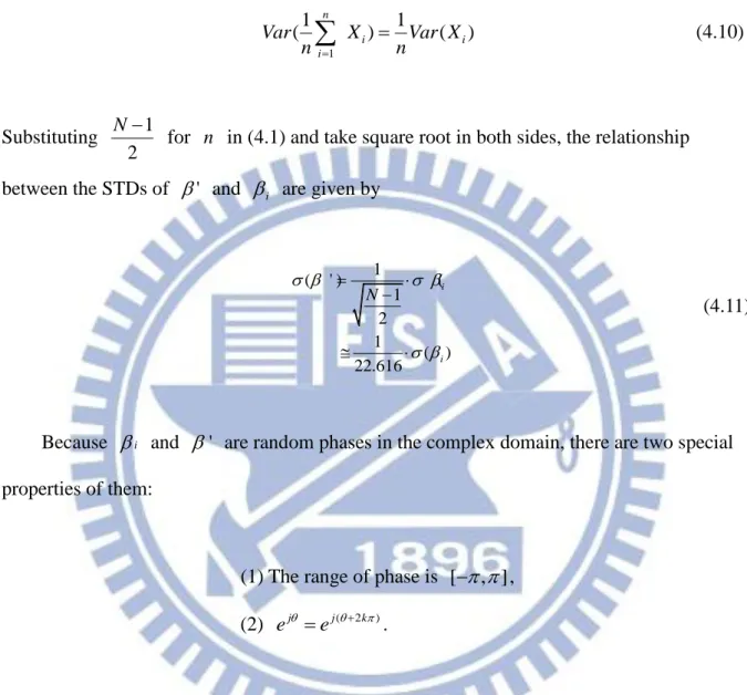
Fig 4.5 shows the STD of q2 in terms of SNR. Obviously, the STD of q2 is much

improved in high SNR cases due to the reduced variance of '. Therefore, after the 2nd estimation we would have an accurate estimation of q for SNR5dB.

Fig 4.5: The standard deviation of q2.

III. Third Estimation

In the third estimation, we use the prior estimation to get a more accurate result. The corresponding k is obtained from₁ round(3)

 , which means the accuracy relies on the prior

estimation of . The equations involved in the third estimation are listed as follows: k₁round(3)  (4.12) 1 1 1 2 ( ) * | | | | j Nk q i i i k i i i k G V V V V e  _       (4.13) 1 1 2 ( ' ) 1 = M _{j k q} j N i i g G g e g e  _   _  



   (4.14) 1 1 2 2 ' h q k N k         (4.15)

For the case of q100 assumed in the simulation, the parameter k is calculated as ₁ 1 3 ( ) 2 3 ( ) 2 3 1023 ( ) 15 2 100 k round q N N round q round         (4.16)

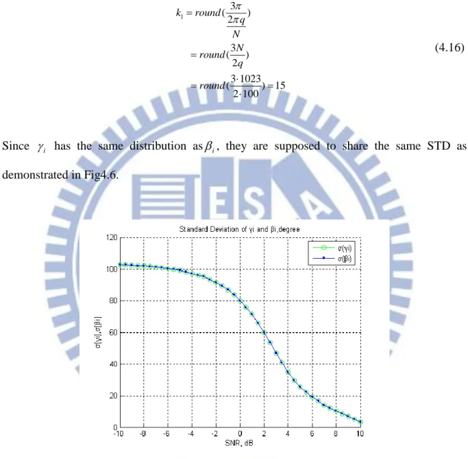
Since _i has the same distribution as_i, they are supposed to share the same STD as demonstrated in Fig4.6.

Fig 4.6: The standard deviations of _i and _i.

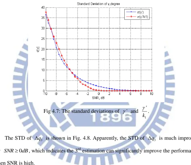
Next, we focus on the ratio of  ( ') to  ( '/k1). The simulation result is shown in Fig 4.7,

where the STD of ' k/ ₁ is reduced when SNR > -5dB. But it even increases when SNR < -5dB. It is because of the undesired mod-2 operation that leads to the increase of  ( '/k1)

in low SNR cases. Recall that k1 is obtained from 3 ( ) round   , which means if 1 2 q k N   is larger than 4 or smaller than2 , the undesired mod-2 operation occurs. From (4.15), we could infer that it will result in increased STD since we add or subtract a factor of

1 2 k  in the calculation.

Fig 4.7: The standard deviations of  ' and

1

'

k



.

The STD of q₃ is shown in Fig. 4.8. Apparently, the STD of q₃ is much improved for SNR0dB, which indicates the 3rd estimation can significantly improve the performance when SNR is high.

Fig 4.8: The standard deviation of q3.

IV. Recursive algorithm

In the third estimation, we figure out that the improvement in estimation accuracy is closely relate to k . And the reliability of 1 k depends on the accuracy of prior estimation. Now, 1

since we have more accurate result after the third estimation, we can proceed to improve the accuracy with the recursive algorithm described before.

In the beginning, we take k k₂ and repeat the process similar to the 3rd estimation as follows: k₂ round(11 ) h   (4.17) 2 2 2 2 ( ) * | | | | j Nk q i i i k i i i k G VV V V e  _       (4.18) 1 2 2 ( ') 1 = M _{j k q} j N i i g G g e g e  _   _  



   (4.19)

2 2 2 2 ' h q k N k         (4.20) The corresponding k should be ₂

2 1 1 ( ) 2 11 ( ) 2 11 1023 ( ) 2 100 56 k round q N N round q round         (4.21)

Fig 4.9: The standard deviation of  ' and

2

'

k



As depicted in Fig 4.9, we find that the performance is still bad when SNR is low, but it is improved for SNR5dB. This result is similar to the 3rd estimation.

The comparison between ('/k1) and ('/k2) is shown in Fig 4.10. Since the

proposed method relies on the accuracy of prior estimation, the relationship between )

/ ' ( k1

 and ('/k2) is not meaningful in low SNR condition. Thus, we merely show the simulation result for SNR010dB. From Fig 4.10, the ratio of ('/k₁) to ('/k₂)

is pretty close to the expected value of 15

56. Recall that a wrong estimation occurs once the deviation is over 2 (0.176 )

2

1 o

N



 , the correct probability of the 4th estimation is much better than that of the 3rd.

Fig4.10: The standard deviation of

1 ' k  and 2 ' k 

Finally, we present the correct probabilities in detecting the code phase with the recursive algorithm with n3,4,5,6 in Fig. 4.11. As shown in the figure, the correct probability is enhanced with the recursive algorithm. Since the recursive algorithm is based on the prior estimation, we can’t increase the correct probability even if we increase the number of iterations in low SNR cases. The result reveals that a more accurate estimation method is needed for the 1st estimation when SNR is low.

Chapter 5

Conclusions

In this thesis, we propose an effective method to achieve code synchronization. In Chapter 2, we introduce basic principle of the FFT method to achieve code synchronization. By performing FFT, the input sequence is projected to the phasor domain, where we get Xi. Then

we compare the phase ofX with the local phasor Yi i. It is found that there is a regular phase

difference within which the code phase q is embedded. Thus we define a factor Vi as the

inner product of Xi and Yi, and it contains information of q. However, due to the inherent

phase ambiguity, we could not interpret the code phase q directly from Vi. Furthermore, we

employ the phasor concept and perform analysis to understand the statistic properties of these phasors.

In general, the sequence length N is a large number. It is known that the computation of FFT and IFFT is in the order of N log N, which means considerable computation is required when the sequence length is long. Therefore, we intend to reduce the computation by using the phase relationship between phasors. By the mathematic analysis, we find every term of Vi

contains information of q, but it can’t be used to get q directly due to inherent phase ambiguity. If we can solve the phase ambiguity problem, the computation caused by IFFT can be saved. Then, by observing the phase of inner product of Vi and Vi+1, we find it contains

information of q without phase ambiguity in noiseless condition. However in noisy condition, the estimation will be strongly affected by noise, which leads to erroneous estimation. In order to improve it, we propose a simple solution to reduce error phase by using the Law of

Large Number.

deviation is larger than 2

N



, a wrong estimation occurs. From the simulation result, even a tiny phase deviation may lead to incorrect value of q. Thus, we propose an improved method to further reduce error phase. By referring to the simple estimation before, we can get the approximated phase angel of Vi*Vi+k. Likewise, when all the terms Vi*Vi+k are summed, we

can obtain a phase whose value is k multiple of q N



2

, and it has the same noise variance as

Vi*Vi+1. Then the variance of error phase is divided by k so that a more accurate estimate is got.

Note that the idea of the improved method can be recursively operated to get more accurate estimation. However, the more estimation the more computation required, so the number of calculations in the recursive algorithm should depend on the SNR.

In Chapter 3 we also design a method to overcome the problem occurring when q is small. It is equivalent to shifting the estimated phase angle to a large value such that the multiplication factor k will not be too large. This method does not reduce noise variance, but requires additional computation. Thus, it is not a necessary process, which is applied only when the estimated phase is close to zero.

In chapter 4, we demonstrate our theory by simulation under different SNR conditions. By analyzing the performance in each step of estimation, we interpret the simulation results and try to overcome the difficulties when SNR is low. Since our method is based on the prior estimation, which means the error may propagate through the process, the only way to enhance the accuracy in low SNR is doing more estimations and costing more computation. In the future, we may design a more accurate method for the 1st estimation, which will improve the performance of the recursive algorithm in low SNR conditions. Moreover, when SNR is known, we can determine the optimum k so as to have the least computation. This n

References

[1] C. Yang, "FFT Acquisition of Periodic, Aperiodic, Puncture, and Overlaid Code Sequences in GPS," Proceedings of the ION GPS 2001, Sept., 2001, Salt Lake City, UT, pp. 137-147.

[2]S. M. Spangenberg, I. Scott, S. McLaughlin, G. J. R. Povey, D. G. M. Cruickshank and P. M. Grant, “An FFT-based Approach for Fast Acquisition in Spread Spectrum Communication Systems,” Wireless Personal Communications, vol. 13, no. 1-2, pp. 27–55, May 2000.

[3] L. Zhao, S. Gao and Y. Hao. “Improved Fast Fourier Transform Processing on Fast Acquisition Algorithms for GPS Signals,’ The Ninth International Conference on Electronic

Measurement and Instruments, vol. 4, pp. 221-224, August 2009, Beijing, China.

[4] N. C. Shivaramaiah, A. G. Dempster and C. Rizos, “Application of Mixed-radix FFT Algorithms in Multi-band GNSS Signal Acquisition Engines ,”Journal of Global Positioning

Systems, vol.8, no.2 .pp174-186, 2009

[5] G. Kolumban, M. P. Kennedy and L.O. Chua, “The Role of Synchronization in Digital Communications Using Chaos - Part I: Fundamentals of Digital Communications, ” IEEE

Transaction on Circuits and Systems—I: Fundamental Theory and Applications, vol. 44, no.

10, pp. 927-936, Oct. 1997

[6] N. F. Rulkov and L. S. Tsimring, “Synchronization Method For Communication With Chaos Over Band-Limited Channel”, International Journal of Circuit Theory and

Applications, vol. 27, pp. 555-567, 1999.

[7] H. Li, X. Cui, M. Lu and Z. Feng , “Dual-Folding Based Rapid Search Method for Long

PN-Code Acquisition,” IEEE Transactions on Wireless Communications, vol. 7, no. 12, pp. 5286-5296, Dec 2008.

[8]H. Li, M. Lu and Z. Feng, “Improved Zero-Padding Method for Rapid Long PN-Code Acquisition,” IEEE Transactions on Signal Processing, vol. 56, no. 8, pp. 3795-3799, Aug. 2008.

Presence of Doppler Shift and Data Modulation,” IEEE Transactions on Communications, vol. 38, no. 2, pp. 241-250, Feb 1990

[10] I. Periˇsa and J. Lindner, “Code Acquisition in Direct Sequence Spread Spectrum Communication Systems Using an Approximate Fast Fourier Transform,” 2006 IEEE Ninth