The effects of environmental factors on the design of master production scheduling systems

(1)

JOURNAL

OF

OPERATIONS

MANAGEMENT

ELS EVIER Journal of Operations Management 11 (1994) 367-384

The effects of environmental factors on the design of master

production scheduling systems

Neng-Pai

Lin

*>a ,

Lee Kraje wskib, G. Keong Leongb, W.C. Bentonb

aNational Taiwan University, 21 Hsu-Chow Road, Taipei, Taiwan

‘Department of Management Sciences, College of Business. The Ohio State University, I775 College Road, Columbus, OH 43210, USA

(Received 10 October 1992; accepted in revised form 1 December 1993)

Abstract

In uncertain environments, firms often use a rolling schedule to implement a master production schedule (MPS). The rolling schedule involves replanning the MPS periodically and freezing a portion of the MPS in each planning cycle. Two important decisions which have a significant impact on the cost performance of a rolling schedule are the choice of a replanning interval (R), which determines the replanning frequency of the MPS, and the selection of a frozen interval (F), which represents the number of periods the MPS is frozen in each planning cycle. The determination of the appropriate F and

R

values has been an important research issue, especially in an uncertain environment.

This paper examines the effects of environmental factors such as cost structure, bill of material (BOM) structure, cumulative lead time, magnitude of MPS change costs, and the magnitude of forecast error on the choice of Fand R for a single end item in an uncertain environment where a rolling schedule is used. Results of our investigation show that the choice of

F

affects total system costs per period (TC) but the effects of the choice of

R

on TC is situational. In addition, the analysis indicates that the magnitude of the MPS change costs, the BOM structure, and the cumulative lead time of the product are important considerations in the design of MPS systems. Results also show that the magnitude of the forecast errors and the cost structure play relatively minor roles in the choice of F and

R.

We also show that even when MPS change costs are high, greater freeze intervals and more frequent replanning may be cost effective.

1. Introduction

The development of a cost-efficient master production schedule (MPS) in uncertain environments is an important issue in many firms that utilize a formal planning system such as material requirements planning (MRP). In an uncertain environment, demand forecasts provide an important input to the MPS. When there are forecast errors, actual demands may not be fully satisfied by production outputs based on the MPS. Two basic options have been proposed to handle problems

*Corresponding author

associated with forecast errors in master production scheduling. The first option is a “rolling schedule” procedure that replans the MPS every period using the newest updated demand data (Baker, 1977). In this approach, MPS changes in each planning cycle induce unstable schedules of components and raw materials through the MRP system, and may incur additional costs. Yano and Carlson (1985) suggest a second option, called “fixed” scheduling, that freezes the timing of production quantities over the entire MPS and keeps enough safety stock to cover the expected forecast errors. Their approach avoids MPS timing changes but increases the inventory holding cost.

(2)

368 N.-P. Lin et al./Journal of Operations Management II (1994) 367-384

Many firms prefer to combine the principles from these two basic options by replanning periodically and freezing a portion of the MPS in each planning cycle. This procedure is also referred to in the literature as a “rolling schedule”. In this paper we adopt the broader definition of rolling schedule defined in Lin and Krajewski (1992). The rolling schedule procedure not only allows for MPS changes but also carries some safety stock for the master schedule item (MSI) to reach a desired customer service level. Two important decisions that affect the performance of the rolling schedule procedure are the choice of a replanning interval (R), which determines the replanning frequency of the MPS, and the selection of a frozen interval (F), which represents the number of periods the MPS is frozen in each planning cycle. The determination of the appropriate values of F and R for an MPS has been an important research issue (Baker, 1977; Lin and Krajewski, 1992; Sridharan et al., 1987, 1988; Sridharan and Berry, 1990a, ‘b; Yano and Carlson, 1987; Zhao and Lee, 1993). However, most studies focus on deterministic environments, and those that consider uncertain environments typically assume that the frozen interval is equal to the replanning interval. Exceptions include Lin and Krajewski (1992) Zhao and Lee (1993), and Sridharan and Berry (1988).

Moreover, several researchers have studied the impacts of the choice of forecast window on total inventory costs of an MS1 in a deterministic environment (Baker, 1977; Carlson et al., 1982; Chung and Krajewski, 1989). The forecast window is defined as the time interval over which the MPS is determined using newly-updated forecast data. The assumption is that both the replanning and frozen intervals are one period. They concluded that the appropriate forecast window for an item depends on its cost structure. Chung and Krajewski (1984) and Sridharan et al. (1987, 1988) addressed the frozen interval issue and show that, in some situations, the MPS should be frozen for more than one period.

Several other articles focus on the MPS in uncertain environments. Sridharan and Berry (1990b) extended the research of Sridharan et al. (1987, 1988) to an environment with uncertain demands.

Specifically, they studied the impact of the forecast window, frozen interval, replanning interval, and methods of freezing the MPS on total cost and size and frequency of MPS changes. In their research they found that there is a tradeoff between safety stock level and MPS changes. Lin and Krajewski (1992) developed an approximation for the average system cost of a rolling schedule procedure for an MSI. The model expressed the average system cost as a function of frozen interval, replanning interval, and other environmental factors. It can be easily used to estimate the cost efficiency for any combination of frozen and replanning intervals, and find the best frozen and replanning intervals. Zhao and Lee (1993) per- formed a comprehensive simulation study and found that forecasting errors can influence the selection of freeze variabies but not replanning frequency and that less frequent replanning improves system performance.

The objective of this paper is to study cost implications of MPS design decisions in uncertain environments where a rolling schedule is used. Managers are concerned with the choices of F and R, and their effects on total expected system cost per period (TC) which includes the forecast error, MPS change, setup, and inventory holding costs. This study examines the effect of environmental factors such as cost structure, BOM structure, magnitude of MPS change cost, and magnitude of forecast error on F and R. A feature that distinguishes this paper from previous research is that an analytical cost model is used as the research vehicle rather than a simulation. This provides us with a more rigorous analysis of the tradeoffs involved.

The remainder of the paper is organized as follows. In the next section, we discuss the master scheduling problem and major decision variables. This is followed by a discussion of the research methodology. Then, we present results of our study. Finally, conclusions are provided.

2. The master scheduling problem

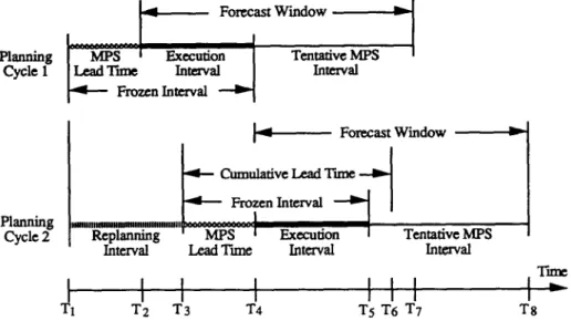
In this study we use a rolling schedule procedure which includes more time intervals than that

(3)

N.-P. Lin et al./Journal of Operations Management II (1994) 367-384

Planning

cycle 2 HIIUIUUlUU~II!IIuullllllll fipl-g ~IL‘;Y$-;-J

Interval Lead Tire Intervi3I Interval

l-ii I

I I I I I I

I I I I I *

Tl T-2 T3 T4 T5 T6 T-I T8

Fig. 1. MPS time intervals in a rolling schedule for a master schedule item.

369

used in past research such as Baker (1977) and Sridharan and Berry (1990a, b). These time intervals will be discussed to get a better understanding of the issues associated with implementing a rolling schedule procedure for the MPS. Figure 1 shows the various MPS time intervals in a rolling sche- dule. The replanning interval(R) is the time interval between two successive replannings of the MPS and determines how often the MPS is replanned. The frozen interval (F) is the time interval over which no schedule changes are allowed. The fore- cast window (T) is the time interval over which the MPS is determined using newly-updated forecast data. The cumulative MSZ lead time (CLT) is the minimum time period required to manufacture the MS1 and procure its raw materials. It is the longest time path of sequential operations and procurement activities in the MSI’s bill of materials, as measured by each component’s lead time. The MPS lead time (L) is the difference between the frozen interval and the replanning (or execution) interval (that is, L = F - R). Notice in Fig. 1 that the MPS lead time is the time interval that overlaps the frozen intervals of two successive planning cycles. Thus, the MPS specified for the intervals T3 to T, in planning cycle 1 remains frozen for planning cycle 2, giving planners a time interval of stability between planning cycles.

The tentative MPS interval is the portion of the

MPS that can be modified in the next planning cycle. An example is the time interval T, to T, in the first planning cycle. The execution interval is the portion of the tentative MPS which is added to the frozen schedule in moving from one planning cycle to the next. Since no updates to the MPS are made during the replanning interval, the con- sumed portion of the frozen MPS must be replaced at the next replanning cycle. Therefore, the execution interval must be equal to the replanning interval.

2.1. Decision variables

The performance of a rolling schedule depends on the choice of F and R. For example, to achieve a certain level of customer service, a firm can freeze a large portion of the MPS to reduce the cost of changes to the schedule and cover demand uncertainties with high levels of safety stocks, or it can freeze a small portion of the MPS and replan more frequently to reduce safety stocks but increase the likelihood of MPS changes. How- ever, the choice of T determines the amount of forward visibility the MPS will provide to the planners of lower-level components and purchased items. From Fig. 1 it is clear that if the firm is to avoid expediting an MPS order every planning cycle, the minimum value of T is a function of the

(4)

370 N.-P. Lin et al.lJournal of Operations Management II (1994) 367-384

cumulative lead time of the MS1 and the choice of to know the cost implications of choosing freeze

Fand R: and review intervals.

T + L L R + max(F, CLT) ₍₁₎

In this study we focus on the freeze and replan-

2.2. Manufacturing environment

ning interval decisions because of their importance to marketing and manufacturing. These functional areas may have different perspectives on the best choice of F and R. The freeze interval determines the stability of the MPS schedule and is a major factor in minimizing the costs of changing the MPS. Manufacturing would like longer freeze intervals to stabilize the environment in support of a market strategy that perhaps places high emphasis on low prices to get customer orders, while marketing might like shorter freeze intervals to allow customer orders to be added or changed on short notice if success in the marketplace depends not only on low prices but also on respon- siveness to customer order changes. The choice of R affects the accuracy of forecasted demand data and the levels of system inventories used to develop the MPS but also affects the frequency of changes to the MPS. Marketing might like more frequent reviews (smaller R) to reflect current market conditions, while manufacturing might favor less frequent reviews (larger R) with larger safety stocks to avoid too many changes. Managers need

This paper focuses on the master scheduling of a single item made to stock in an uncertain environment using a rolling schedule. Specifically, we examine the effect of F and R on the total system costs on the manufacturing environment described in Table 1. This environment is consistent with much of the literature in MPS system design (Benton and Srivastava, 1985; Blackburn and Millen, 1982; Lin and Krajewski, 1992; Sridharan and Berry, 1988; Sridharan et al., 1987; Yano and Carlson, 1985; Zhao and Lee, 1993).

There are several points of departure from the previous MPS research. First, a modified POQ (periodic order quantity) rule is used to determine the MPS quantities. It is modified to account for the effects of forecast errors on actual inventory levels in the first lot sizing decision in a planning session. This allows the system to refurbish lost safety stocks or avoid overproduction if expected demands did not materialize each planning session. We use the POQ rule because it has been proven to perform well in an uncertain demand environment (Lee and Adam, 1986) and

Table 1

The manufacturing environment Demand Forecast errors Capacity constraints Number of MS1 Service level MPS procedure Lot-sizing rule

Uncertain; discrete; follows a distribution with known mean and variance; identical and independent distribution from period to period; no trends or seasonalities.

Unbiased forecast; distribution of errors in each period has a mean of zero and a standard deviation that is an increasing function of the number of periods into the future.

No capacity constraints on the production of the master scheduled item (MSI) and its components; all purchased materials available.

One, made to stock.

Defined as the probability of not running out of stock over the freeze interval; determined a priori; is used to determine the safety stock of the MSI; demand backlogged in one period is satisfied on a first-come first- served basis in the next period.

MPS is developed using a rolling schedule procedure; lot size rule and the frozen, replanning and forecast window intervals are chosen a priori and fixed; forecast the demand within the forecast window; determine the MPS within the forecast window using the lot size rule; authorize the MPS in the execution interval; roll ahead in time to the end of the replanning interval to make the next forecast.

POQ rule for the lot sizes within the forecast window; the first lot size in a planning session is adjusted to account for backlogged demand in the previous review interval and current inventory levels; time between orders is based on the MSI’s natural cycle.

(5)

N.-P. Lin et al./Journai

of

Operations Management II (1994) 367-384 371

Wemmerlov (1979) found it to be one of the most popular lot-sizing rules of MRP users. In addition, differences between lot-sizing rules tend to be less significant as demand uncertainty is introduced (Sridharan et al., 1988; Benton and Whybark, 1982). Moreover, a preliminary study by Lin (1989) found that the POQ rule significantly reduced MPS changes when compared to the WagnerWhitin rule.

error costs, MPS change costs, and setup and holding costs. Details on the derivation of the MPS model can be found in Lin and Krajewski (1992) and Lin (1989). The cost functions, back- ground comments on each one, and a complete list of all the notation are contained in the Appendix.

Second, the lot-for-lot rule is used for all components and assembly lot sizes. This is a simplifica- tion, but allows us to directly reflect the effects of MPS changes on the components and subassemblies.

Forecast error costs

Third, our rolling procedure differs from past research such as Baker (1977) and Sridharan and Berry (1990a, b). The MPS is replanned every R periods. At the start of each replanning period, existing unfrozen orders are adjusted and new orders are placed to cover updated demand fore- casts within T. Both the timing and the quantities of production orders are frozen over the interval F. Safety stocks are used to satisfy unexpected demand. All component schedules supporting the frozen MS1 schedule are similarly frozen, but unfrozen schedules (both components and MSI) can be changed at a cost which is a function of the size of the change and the length of the time interval until the change is needed. The MPS procedure is given in Table 1. Details can be found in Lin and Krajewski (1992).

The forecast error costs are the costs of holding sufficient safety stock to satisfy a given cycle service level requirement. The safety stock needs to cover F periods and depends on the standard deviation of forecast errors over that time interval, which in turn depends on the forecast error variance function and the review interval, R. Consequently, the forecast error costs are a function of the per-unit holding costs, F, R, and the forecast error variance function, which can be any mathematical expression depicting the variance of forecast errors as a function of time.

MPS change costs

3. Research methodology

Estimating total system costs in the manufacturing environment described in Table 1 requires a specification of the complex relationships between the relevent environmental factors and the decision variables that define the master scheduling process. In this study we use a cost model developed by Lin and Krajewski (1992) that estimates the total system costs for any combination of F, R, and T and subject it to a variety of scenarios to gain insights to the tradeoffs involved in the design of MPS systems.

The MPS within the tentative MPS interval may be changed as the MPS is rolled ahead. In the MPS

model, these changes represent increases or

decreases in lot sizes and not changes in the timing of production lots. This is consistent with an environment where the product is made to stock and

unexpected demands are covered with safety

stock. In this situation, increases in MPS lot sizes can cause additional setups, expediting, increased

procurement costs, component shortages, or

“pirating” of components from another product. Decreases to MPS lot sizes can cause inventories of components to rise and increased idleness due to disrupted schedules. The MPS change costs

depend on a “unit” change cost function

(explained later) that is constructed from the MSI’s bill of material and routings, and the standard deviation of MPS quantity changes, which is a derived function of L, R, the forecast error variance function, and the time between orders.

3.1. MPS model

Setup and holding costs

The MPS model consists of three cost functions The expected setup and holding costs depend which comprise the total system costs: forecast on the time between orders of the POQ system,

(6)

312 N.-P. Lin et al./Journal of Operations Management II (1994) 367-384

setup costs, and the unit inventory holding Table 2

costs. Environmental factors

3.2. Evaluation of the MPS model

It is important to note that the MPS model contained in the Appendix utilizes cost functions derived from continuous probability distributions to estimate the expected costs of rolling schedules in an environment with discrete demands and order quantities. The quality of the MPS model’s estimates was thoroughly tested by comparing them to those generated from a simulation model using discrete demands and order quantities and the MPS procedure described in Table 1 (Lin, 1989). Sixteen manufacturing environments were generated by systematically adjusting factors such as cost structure, BOM structure, unit change cost functions and forecast error variance functions. The simulation of each manufacturing environment was replicated five times. The safety stocks recommended by the MPS model for a target cycle service level of 90 percent were used by the simulation model and the resultant cycle service levels were calculated after 4000 periods of steady-state simulation. The actual (simulated) service levels ranged from a low of 89.1 percent to a high of 90.7 percent. In addition, the MPS model’s cost estimate for the best combination of F and R was within 1 percent of the simulation’s cost and within 0.4 percent in all but one case. Finally, the MPS model matched the best combi- nation of F and R found with the simulation in all but one case. For that case, the total system costs were only 0.2 percent higher than that of the simulation.

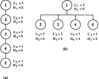
(a) BOM structure

Simple: as shown in Fig. 2(b); CLT = 12, and U(u) = (Yu, (u)

Complex: as shown in Fig. 2(a); CLT = 2 1, and U(u) = &J,(u)

(b) Magnitude of unit change cost Low: ru = 0.2

High: o/ = 2.0 (c) Magnitude of forecast error

Low: c,(u) = 0.15u High: D,(U) = O.l5u’3

associated with MRP nervousness induced by a one-unit change in the MPS. However, the degree of MRP nervousness depends on the BOM structure of an MSI. A complicated BOM structure with many levels may cause more system nervousness and more MPS change costs than a simple BOM structure. Consequently, the unit change cost function is dependent on the BOM structure. Therefore, the three environmental factors in our study are: BOM structure, magnitude of unit change cost, and magnitude of forecast error. Each factor has two levels, as shown in Table 2, yielding a total of eight environments.

BOM structure

Two MSIs with extreme BOM structures shown in Fig. 2 are selected for testing the MPS model. These two BOM structures have been used by Graves (1981) Blackburn and Millen (1982), and

Benton and Srivastava (1985). The two BOM

structures have their own CLTs and unit change cost functions (U(u)).

3.3. Environmental settings

The purpose of this study is to investigate a variety of scenarios so managers can have a better understanding of the cost implications of MPS process design strategies in a wide range of operating environments. Two important factors that have direct impact on the MPS change cost and forecast error cost are the unit change cost function and the forecast error standard deviation function. The unit change cost function describes the cost

In this study, the CLT of the MS1 is defined as the time interval from the planning of the procurement of raw materials to the completion of the MS1 and includes not only the lead time for procurement/manufacturing, as used in previous research (Baker, 1977; Sridharan and Berry, 1990a, b), but also the proper planning horizon for the lot-sizing decisions of the components. The reason is that without adequate forward visibility, the lot-sizing decisions of components may have high setup and inventory holding costs. The proper planning

(7)

N.-P. Lin et al./Journal

of

Operations A4anagement II (1994) 367-384 373 1

Q

L’, =3 H, =0

Q

1 _{HI =O}L’, =3 L’4=3 H4=0 L’s=3 H5 =6 (a)

Fig. 2. Bills of material (LJ is the manufacturing/procurement lead time for item j; H, is the planning horizon for item j).

horizon for an item depends on the demand pattern, lot-sizing rules used, and the associated cost structure for the entire operating system.

In Fig. 2, item 1 represents the MS1 in both cases. The planning horizons for the MS1 and all inter- mediate items in our example are zero because the lot-for-lot rule is used for all components and the standard lead time offsetting will allow sufficient forward visibility to make good lot sizing decisions. The planning horizons for the raw materials are also shown in Fig. 2. In Fig. 2(a), the cumulative lead time of the MS1 equals the sum of the manufacturing/procurement lead times (LI) and planning horizons (Hj) for items 1, 2, 3, 4, and 5. Thus, the CLT of the MS1 is equal to (3+ 3 + 3 + 3 + 3 + 6) which is 21. When the MS1 has more than one component, as shown in Fig. 2(b), the cumulative lead time of the MS1 equals:

Cumulative lead time

= maximum{l{ + Ht + (Lj + Hj)},

j = 2,3,4,5.

Consequently, the cumulative lead time of the MS1 in Fig. 2(b) equals [maximum ((3 + 3 + 6), (3 + 3 + 4), (3 + 3 + 4), (3 f 3 + 6)}], which is 12.

Magnitude of unit change cost

Even though the BOM structure is kept the

same, the unit change cost function of an MS1 may be affected by reducing the setup and inventory holding costs of its components. In order to include this situation, we let the unit change cost function, U(u), equal a fixed function multiplied by a factor, cr, called the magnitude of unit change cost. In the simple setting of the BOM structure, the unit change cost function is:

U(u) = oU1 (u), (2)

where

U,(u) =

10 - 1.27(u - 3) 3 < u < 10, l.lll-0.555(u-10) lO<u< 12,

12 < u. In the complex BOM setting, the unit change cost function is:

U(n) = QJJ2(u), (3)

where

(m u < 3,

U,(u) = 10 - 0.833(u - 3) 36u6 12, 2.5 - 0.278(u - 12) 12 < u < 21,

21 du.

The unit change cost function for an MS1 is developed by accumulating the change costs for each of its components, recognizing lead time offsets (Lin, 1989). Consequently, U(u) is a reflection of what it would cost to make a one-unit change to the MPS u time periods in the future. MPS change costs are calculated by multiplying the expected size of the MPS change by the unit change cost function. For example, in the simple setting of the BOM structure, the MS1 itself has a manufacturing lead time of three periods, but each of its components also have lead times of three periods plus varying planning horizon offsets. The total CLT is twelve periods, but the cost of changing the MPS is greater only a few periods in the future than it is closer to twelve periods out. The purpose of the unit change cost function is to reflect these cost differences. Suppose that Q = 0.2. The MPS change cost for increasing the MPS by fifteen units eight periods in the future would be 0.2[10 - 1.27(8 - 3)](15) = 10.95. Changes eight

(8)

374

Table 3

N.-P. Lin et a/./Journal of Operations Management I1 (1994) 367-384

Coefficient of variation ratios

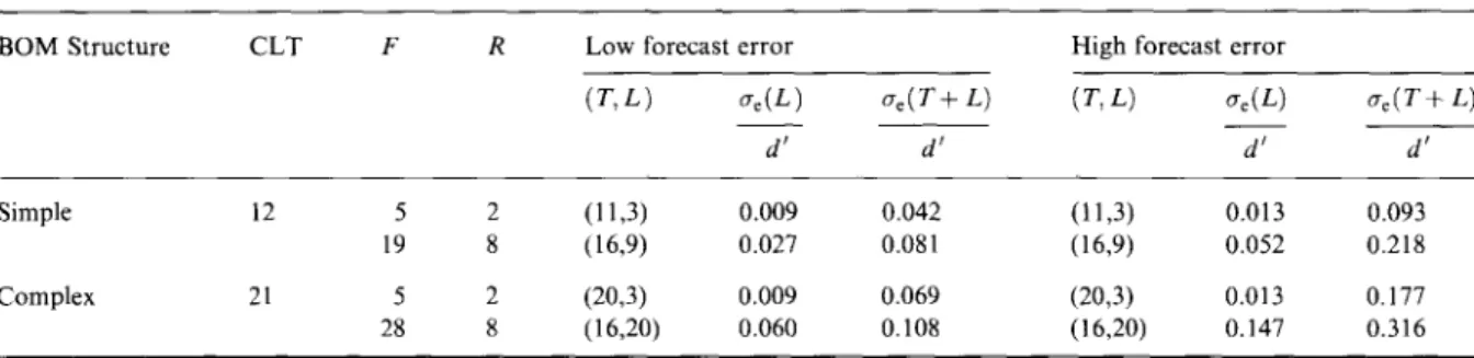
BOM Structure CLT F R Low forecast error High forecast error

(T>L) G(L) dT+ L) (T, L) G(L) dT+ L) d’ d’ d’ d’ Simple 12 5 2 (11,3) 0.009 0.042 (11,3) 0.013 0.093 19 8 (16,9) 0.027 0.081 (16,9) 0.052 0.218 Complex 21 5 2 ~3) 0.009 0.069 (20,3) 0.013 0.177 28 8 (16,201 0.060 0.108 (16,201 0.147 0.316

periods in the future affect the procurement quan- selected two functions to depict two very different tities of items two through five in this case. This is situations in Table 2. In both cases the forecast obviously an approximation to the actual costs in a standard deviation is a function of the time inter- situation which may involve fixed costs such as val u. The low setting depicts scenarios where the setups. Nonetheless, our approach of approxi- standard deviation of forecast errors increases mating these costs on a per-unit basis is analogous linearly as a function of u. The high setting repre- to the approach used in the capacity bills or resource sents high forecast error situations where the

requirements planning methods for capacity standard deviation of forecast errors increases

planning in MRP systems (Vollman et al., 1992). exponentially with u. In practice, many companies use time fencing to

establish guidelines for the kinds of changes that can be made in various period (Vollman et al., 1992; Berry et al., 1979; Pohlen, 1985). The cost of making changes within the first time fence of an item, which conceivably could be the components normal lead time, is set to an extremely large number (M) to discourage changes. In subse- quent time fences, the penalty for making changes becomes progressively less severe. The procedures to derive the functions U,(u) and U,(u) have been provided in Lin (1989).

Two values are selected for parameter CY. The value of cy equals 0.2 in the low setting, and 2.0, which is double of the normal situation, in the high setting. While the value of these parameters were chosen arbitrarily, we consider this range of (Y sufficiently large to cover many reasonable situations.

Magnitude of the forecast error

The magnitude of the forecast error is represented by the forecast error standard deviation function, gee(u). In this study, the standard deviation of forecast errors increases the farther in the future the forecast is projected. While the MPS model can use any function for a,(u), we have

This forecast error factor is different from previous research on master production scheduling where the forecast error standard deviation (S’) is assumed to be independent of time and fixed for all periods. Specifically, Yano and Carlson (1985, 1987) used three values for S’ such that the corresponding coefficient of variation ratios of

S//d’ equalled 0.05, 0.15, and 0.25 respectively. Sridharan et al. (1988) used two values of S’ so that coefficients of variation equalled 0.15 and 0.3. A single value for S//d’ is not appropriate in our study because a,(u) is a function of time. Specifically, the choices for F, R, and T and the factor setting for the BOM structure determine the range of forecast error distributions to be addressed by the MPS model. Refer to Fig. 1 and planning cycle 1. In period Tt a forecast must be made for each period in the interval T2-T,. For period T2, the forecast error standard deviation will be o,(L). For period T, it will be a,(T+ L),

the maximum value for the particular choice of T and L. The values of T and L must adhere to the relationship in (1).

Table 3 contains the coefficient of variation ratios for the extreme values of F and R explored for each BOM structure setting. The value of d’ is 50 units per period. Although the relationships

(9)

N.-P. Lin et al./Journal of Operations Management 11 (1994) 367-384 375

implied in Table 3 are more complex than those reported in other studies, the values for the coefficient of variation at the extremes compare favorably to the static values used by Yano and Carlson (1985, 1987) and Sridharan et al. (1988).

Fixed factors

In all eight environments studied, the cost structure, the standard deviation of the demand distribution (a), and the cycle service level (g) are fixed. The cost structure is selected such that the natural cycle of the MSI, as defined by Baker (1977) is equal to two. The value of 0 is based on previous research. For example, Blackburn and Millen (1982) select the value for u such that (o/d’) equals 0.2. Sridharan et al. (1987) use three values for 0 such that (a/d’ ) equals 0.1443, 0.2165, and 0.433. In our environment, D equals 10 and (a/d’) equals 0.2. The value of u is fixed because the forecast is unbiased and, therefore, it is forecast errors and not the standard deviation of demand that affect costs. Preliminary experiments indicate that the relationship between F, R, and total costs (TC) are unaffected by values of g ranging from 60% to 95% (Lin, 1989). Conse- quently, g is fixed at 90%.

3.4. Search procedure

The MPS model can estimate the total system costs for any combination of F and R subject to the logical condition that R must never be greater than F. The forecast window can be any value satisfying (1). The number of potential combina- tions is large. However, for the purposes of the discussion to follow, we will limit the search so that we can focus on the cost implications of the choice of F and R. In particular, we restrict T in each manufacturing environment to be the smallest value that is an integral multiple of the MSI’s natural cycle satisfying (1). This allows the forecast horizon to cover an integral number of production lots since the POQ rule we are using covers the MSI’s natural cycle (see Table 1). In addition, this allows us to focus on the choice of F and R while using a reasonable forecast window. We also restrict the values of R to be integral multiples of the MSI’s natural cycle. Preliminary

investigations (Lin, 1989) indicate that in uncertain environments the MPS changes increase signiti- cantly when R is not an integral multiple of the natural cycle. This is a consequence of the particular POQ rule used in this study. The MPS model is not restricted to these conditions on T, R, and the POQ rule.

4. Insights into the design of MPS systems

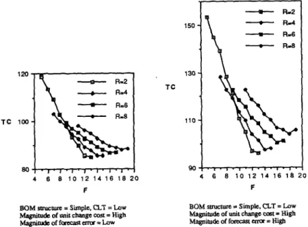
The effects of the choices of F and R on the total expected system costs per period (TC) for the eight

environments with the assumptions described

earlier are shown in Figs 3(a)-(d). Several generali- zations about the effects of the choices of F and R on TC can be observed. The factors that appear to have a considerable impact include the cumulative lead time of the product, the magnitude of the MPS change costs represented by o, and the

BOM structure. A summary of the findings,

based on comparisons of Figs 3(a) through (d), are presented below.

- Total expected system cost per period is more sensitive to the choice of frozen interval (F) than to the replanning interval (R).

- As the frozen interval decreases, the replanning interval tends to increase for complex BOM structures.

- The magnitude of forecast errors has no effect on the best combination of F and R, but the total expected system cost per period is more sensitive to the choice of F when forecast errors are high.

- When MPS change costs are high, the frozen interval (F) should be at least as long as the cumulative lead time of the product. When MPS change costs are low, make F as small as possible.

~ With a short cumulative lead time (BOM structure in Fig. 2(b)) and high MPS change costs, the choices of both the replanning and freeze intervals are critical. With a long cumulative lead time (BOM structure in Fig. 2(a)), the choice of the frozen interval alone is critical.

- When MPS change costs are low, the cumulative lead time of the product has little effect on the choice of optimal frozen and replanning intervals.

(10)

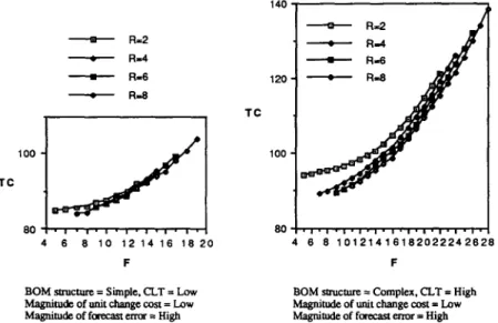
376 N.-P. Lin et al./Journal of Operations Management II (1994) 367-384 TC 100 - FL6 4 6 6 10 12 1416 16 20 F 130 TC 6 6 10 12 14 16 16 20 F

BOMSINC~IV= Siiple,CLT=Low BOM suuchue = Simple, CLT = Low h&@& ofunirchangecoa=High ~agnitudcofunitchangcccst=High

h.fa@nldeoff~wr=~ Mag&deoffo~tam= High

Fig. 3(a). Effects of F and R on TC for a change in the forecast error.

4.1. Discussion

The results from these environments may not hold

in other environments where there are capacity

constraints or demand patterns other than that

used in this study. Nevertheless, these results may

be helpful in understanding

the issues involved

in designing MPS systems. The fundamental

TC 60 TC - R-2 -R-4 --CR-6 -R-6 4 6 6 10121416162022242626 170 - R-2 - R-4 150 - R-6 - R=8 130- 110’

901

4 6 6 10121416162022242626 F F

BOM stature = Complex. CLT = High BOM structure = Complex, CLT = High MqniN&eofurlitehangecosl=Lw Magnitude. of unit change cosl = High Magnitudeoff-erru=l&v Maqimde of forecast error = Low

(11)

N.-P. Lin et al./Jomnal of Operations Managemen If (1994) 367-384 377 TC 180 160 140 120 4 6 8 10 12 14 16 18 20 F

BOM structure = Complex, CLT = High BOM smtcture f Simple, CLT 5 IXW Magnitude of unit change. cost = High Magnitude of unit change cost = High Magnitude of fonxast anx 9 High Magnitude of fotecast mur = High Fig. 3(c). Effects of F and R on TC for changes in BOM structure with high unit change costs

question is: Are the choices of

F

and R important?

The results show that the value of TC depends on

the value of

F

in all environments investigated in

this study. Also, TC is more sensitive to the choice

of

F

when forecast error increases. It appears that

managers need to choose an appropriate

F

for the

MPS.

The effect of the choice of R is complex, It

depends on the magnitude of unit change cost

and the values of

F

and CLT. When the magnitude

of unit change cost is high and CLT is low (see Figs

3(a) and 3(c)), the choice of

R

has important effects

on TC, regardless of the value of

F.

However, when

the magnitude of unit change costs is low

or

CLT is

high (see Figs 3(b)-(d)), the effect of the choice of

R

depends on the value of

F.

In either of these situa-

tions, when

F

is small relative to CLT, replanning

frequently (R = 2) causes relatively higher TC. This

result is consistent with the findings in previous

research, such as Yano and Carlson (1985) and

Sridharan et al. (1988). On the other hand, when

F

is large, the choice of

R

has minor effects on TC.

The results also demonstrate

the effects of

environmental

factors. The magnitude

of unit

change cost affects the best choice of

F

and R in a

significant way. When the unit change cost is

high, the results indicate that we should freeze

longer intervals to reduce the MPS change costs.

(12)

378 N.-P. Lin et al./Journal of Operations Management 11 (1994) 367-384 140 -. - F&z - R=2 _{. -} _R-4 - R-4 - R-6 - R-6 120- - R-8 - R-8 TC 4 6 8 10 121416 1820 4 6 8 10121416182022242628 F F

BOM s&ucturc. = Simple. CLT = Low BOM structure = Complex, CLT = High Magnitude of unit change cost = Low Magnitude of unil change cost = Low MagnibJde of fa-ecast errcu = High Magnihzde of f- error = High

Fig. 3(d). Effects of F and R on TC for a change in the BOM structure with low unit change costs Consequently, the optimal frozen interval for

the environments with a high value of LY is larger than that for the environments with a low value of a. On the other hand, the results from these experiments suggest that the magnitude of the forecast error has minor effects on the best choice of F and R. If the standard deviation of forecast errors changes modestly, managers can keep the same F and R for the MPS.

The result that the forecast error has minor effects on the best choice of F and R may surprise managers. Intuitively, managers may expect a shorter frozen interval for higher forecast errors because more safety stock is required for a given frozen interval when the forecast errors are higher. However, the best combination of F and R in an environment is the one that balances the MPS change cost and forecast error cost simultaneously. When forecast errors increase, they increase the required safety stock and the size of MPS changes, thereby increasing both the safety stock costs and the MPS change costs. Total costs therefore increase, but the best choice of F and R remains about the same.

5. The effects of MPS change costs on MPS system design

It is apparent from our previous analysis that

MPS change costs are an important consideration in the design of MPS systems. To explore this issue further, we conducted another experiment, retain- ing two of the factors from the first experiment and adding a new one: cost structure.

The values of cost structure and magnitude of forecast error are fixed in two settings: low and high. The cost structures are selected such that the natural cycle of the MS1 is equal to two in the low setting and four in the high setting. The settings for the magnitude of forecast error are identical to the low and high settings in Table 2. The BOM structure is fixed in all environments but the magnitude of the unit change cost is changed. The fixed BOM is similar to the high setting in Table 2 except that the value of CLT is 17, the average of the low and high settings for this factor. The new unit change cost function, U(u) is provided below:

U(u) = aU3(u), where (4) U,(u) = 1 M u < 2.4, 10 - l.O27(u - 2.4) 2.4 < u < 9.7, 2.5 - 0.343(u - 7.3) 9.7 < u < 17, 0 17 < I.4

The graph of the unit change cost function, U3 (u) is shown in Fig. 4.

(13)

N.-P. Lin et al./Journal of Operations Management 11 (1994) 367-384 319

0 5 10 15 20 25

u

Fig. 4. Unit change cost function U,(u)

The changes to the magnitude of the unit change cost are made by changing the values of the parameter cy by 0.2 each time from 0.2 through 2.0. The MPS model is used to determine the best combination of F and R for all resulting environments.

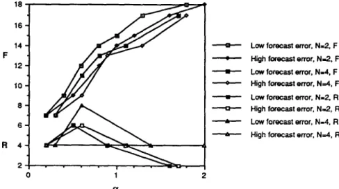
The results are displayed in Fig. 5. The horizon- tal axis demarks the values of cy while the vertical axis represents the number of periods for the best F and R for each value of CL Sometimes, several sequential values of o resulted in the same F or R. In these cases, we plotted a single point for F or R at the average of the value of Q that generated it. This approach simplifies the lines in Fig. 5 but still keeps the essence of the relationship we wish to examine.

The frozen interval (F) increases steadily as the

18

16

6 6 R 4

magnitude of the MPS change costs increases. This is a logical result given the desire to avoid changes in the MPS even though the resulting forecast errors will cause increased safety stocks (see Appendix, Forecast error cost).

The behavior of the replanning interval (R) is more difficult to explain. Intuitively, when MPS change costs are high, replanning should be kept to a minimum to avoid changing the MPS. How- ever, in our experiment, R increases for increases in the magnitude of MPS change costs, then decreases as the change costs get very large. There is a complex interaction of cost factors at work. Refer to Figs 1 and 4. Given the unit change cost function, if MPS changes must occur, it is desirable to make them in periods as far out in the future as possible. As R (the execution interval as well as the replanning interval) gets smaller for a given F, we add smaller pieces of the tentative MPS interval to the frozen part of the schedule. Furthermore, these additions occur further out in the future, where it is cheaper to make changes according to the unit change cost function. In our experiment U,(u) has a kink at 9.7 periods (see Fig. 4 and equation set (4)). The location of the kink is a function of the BOM we are using and the specific costs to make MPS changes at various points in the manufacture of the MSI. In general, there may be more kinks, or none at all, depending on the costs and BOM involved. In our present case, when MPS change

v Low forecast error, N=2, F

--t- High forecast error, Nd. F --m- Low forecast error, N=4, F - High forecast error, N=4. F --m- Low forecast error. N=2. R I High forecast error. N-2, R -)- Low forecast error, N-4. R - High forecast error, N=4. R

(14)

380 N.-P. Lin et al./Journal of Operations Management I1 (1994) 367-384

costs get too large, we will want to keep MPS lead time (L =

F - R)

above 9.7 to keep MPS change costs down. Consequenty, as MPS change costs increase (a),

F

increases and

R

keeps pace, leaving

L

unchanged. Further increases in a require a larger

L

(to move further down the unit change cost function to the kink) which can be accom- plished by increasing

F

and holding

R

constant. Finally, the MPS change costs get so high that

F

increases

and

R

decreases to increase

L

beyond the kink more quickly.

The behavior of

F

and

R

in Fig. 5 is a function of complex tradeoffs in the forecast error and MPS change cost elements of the MPS model (see Appendix). For our experimental settings, for a > 0.6,

R

decreases as MPS change costs rise

because the unit change cost function

(U(L + ( j - l)M)) decreases faster than the vari-

ance of the MPS change distribution (S,“)

increases. The net effect is a reduction in the expected MPS change cost (C,). In addition, reducing

R

regardless of the value of cy results in a lower variance of the safety stock distribution (0;) and hence lower safety stock costs. Combined, total costs go down. For CY < 0.6, increasing

R

is better because reductions in 5’: dominate the increases in U(L+ (j- l)M) and a:.

The implication for the design of MPS systems is clear. The magnitude of the MPS change costs as well as the shape of the unit change cost function play an important role in the choice of

F

and

R.

The shape of the unit change cost function depends on the BOM structure, including all component lead times. We have demonstrated that even when MPS change costs are high greater freeze intervals and more frequent replanning may be cost effective. This is a function of the product structure (BOM) and MPS change costs. In our experiments the cost structure factor did not play a noticeable role.

6. Conclusion

Most studies on MPS have focused on deterministic environments and those that consider uncertain environments typically assume that the

frozen interval is equal to the replanning interval. In this research, we have used a rolling schedule which included more time intervals than that used in past research. We examined several operating environments to provide managers with a better understanding of the implications of the design of MPS systems on costs.

We have investigated the effects of the choices of

F

and

R

on TC and found that the choice of

F

affects TC, but the impact of the choice of

R

on TC was situational. We also examined the impact of environmental factors on the design of MPS systems and found that the magnitude of the MPS change costs as well as the shape of the unit change cost function play an important role in the choice of

F

and

R.

Additionally, our analysis showed that even when MPS change costs are high, greater freeze intervals and more frequent replanning may be cost effective. While results from this study may not be generalized to other environments, they may be helpful in understanding the issues involved in the design of MPS systems.

Research into the design of effective MPS systems is still in its infancy. Models such as the one used in this study at best identify issues that should be explored in more realistic settings. Future research might address the limiting environment that the MPS model is based on. For example, models that include many end items, seasonal demand patterns, and recognize critical capacity constraints would be useful. Moreover, new work needs to be done on the MPS change cost function, identifying ways to reflect the costs of MPS changes in real manufacturing settings. Finally, the design of MPS systems needs to be better related to the market strategies of the firm, and be able to address make-to-stock as well as

assemble-to-order environments. We need to

address the issue of coping with widely different market segments.

References

Baker, K.R. 1977 “An experimental study of the effectiveness of rolling schedules in production planning”. Decision Sciences,

(15)

N.-P. Lin et al./.Journal

of

Operations Management II (1994) 367-384 381

Benton, W.C. and Srivastava, R., 1985. “Product structure complexity and multilevel lot sizing using alternative costing policies”. Decision Sciences, vol. 16, no. 4, 3577369. Benton, W.C. and Whybark, D.C., 1982. “Material Require-

ments Planning and purchase discounts”. Journal of Operations Management, vol. 2, no. 2, 1377143.

Berry, W.L., Vollmann, T.E., and Whybark, D.C., 1979. Master Production Scheduling: Principles and Practice. American Production and Inventory Control Society, 1979.

Blackburn, J.D. and Millen, R.A., 1982. “The impact of a rolling schedule in a multi-level MRP system”. Journal of Operations Management, vol. 2, no. 2, 125-135.

Carlson, R.C., Beckman, S.L., and Kropp, D.H., 1982. “The effectiveness of extending the horizon in rolling production scheduling”. Decision Sciences, vol. 13, no. 1, 1299146. Chung, C.H. and Krajewski, L.J., 1984. “Planning horizons for

master production scheduling”. Journal of Operations Management, vol. 4, no. 4, 389-406.

Chung, C.H. and Krajewski, L.J., 1986. “Replanning frequen- cies for master production scheduling”. Decision Sciences,

vol. 17, no. 2, 263-273.

Graves, S.C., 1981. “Multi-stage lot-sizing: An interactive procedure”. In: L.B. Schwarz (Ed.), Multi-level Production] Inventory Control Systems: Theory and Practice. North- Holland, Amsterdam, 1981, Chap. 4.

Lee, T.S. and Adam, E.E., 1986. “Forecasting error evaluation in Material Requirements Planning (MRP) production- inventory systems”. Management Science, vol. 32, no. 9,

118661205.

Lin, N.P., 1989. “Master production scheduling in uncertain environments”. Unpublished doctoral dissertation, The Ohio State University, 1989.

Lin, N.P. and Krajewski, L.J., 1992. “A model for master production scheduling in uncertain environments”.

Decision Sciences, vol. 23, no. 4, 8399861.

Pohlen, M.F., 1985. “The freeze fence: The balancing point between management strategy and operating control”.

APICS I985 Conf Proc., pp. 66-69.

Sridharan, V. and Berry, W.L., 1988. “An analysis of the cost-schedule stability trade-offs for freezing the master production schedule under uncertainty in a rolling schedule environment”. Decision Sciences Institute Nat. Conf. Proc.,

Las Vegas, 1988.

Sridharan, V. and Berry, W.L., 1990a. “Master production scheduling make-to-stock products: A framework for analysis”. International Journal of Production Research,

vol. 28, no. 3, 541-558.

Sridharan, V. and Berry, W.L., 1990b. “Freezing the master production schedule under demand uncertainty”. Decision Sciences, vol. 21, 977120.

Sridharan, V., Berry, W.L. and Udayabhanu, V., 1987. “Freezing the master production schedule under rolling planning horizons”. Management Science, vol. 33, no. 9,

113771149.

Sridharan, V., Berry, W.L., and Udayabhanu, V. 1988. “Measuring master production schedule stability under rolling planning horizons”. Decision Sciences, vol. 19,

no. 2, 1477166.

Vollman, T.E., Berry, W.L., and Whybark, DC., 1992,

Manufacturing PIarming and Inventory Control Systems.

Richard D. Irwin, Homewood, IL, 1992.

Wemmerlov, U., 1979. “Design factors in MRP systems: A limited survey”. Production & Inventory Management, vol. 20, no. 4, 15-35.

Yano, CA. and Carlson, R.C., 1985. “An analysis of scheduling policies in multiechelon production system”. ZZE Trans- actions, vol. 17, no. 4, 370-377.

Yano, CA. and Carlson, R.C., 1987. “Interaction between frequency of rescheduling and the role of safety stock in Material Requirements Planning systems”. International Journal of Production Research, vol. 25, no. 2, 221-232.

Zhao, X. and Lee, T.S., 1993. “Freezing the master production schedule for material requirements planning systems under demand uncertainty”. Journal of Operations Management, vol. 11, no. 2, 185-205.

Appendix-Costs included in the MPS model The expected system cost in the MPS model includes the forecast error cost, MPS change cost, and setup and inventory holding costs. A brief explanation of these costs is provided below. The notation we use is contained in Table A.1. A detailed explanation of the derivation of these costs is presented in Lin and Krajewski (1992).

A.I. Forecast error cost

(1) The forecast error cost is defined to be the cost of carrying the safety stock required to satisfy the cycle service level.

(2) The forecast error for some future period t has a normal distribution with mean of zero and standard deviation of Us, where u is the time interval between the current period and period t. The function a,(u) can be of any mathematical expression, however, we assume that the value of a,(u) gets larger as the time interval u increases.

(3) The standard deviation of total forecast error over the frozen interval is a function of F and R.

(4) Given a fixed cycle service level g, the forecast error cost per period, CF, is:

(16)

382 N.-P. Lin et al./Journal

of

Operations Management 11 (1994) 367-384

Table A. I. Notation

Time

T = Forecast window interval.

R = Replanning interval; also the execution interval

L = MPS lead time interval. F = Frozen interval; equals R + L.

M = Number of time periods between orders for the modified POQ rule; equals the MSI’s natural cycle. u = Number of periods between the current period and a specified future period.

L; = Production lead time for item j, where j = 1 is the MS1 and j # 1 are components.

Demand

d’ = Mean of the frequency distribution for demand.

o:(u) = Forecast error standard deviation function for forecasts of demand u periods in the future.

CF = Standard deviation of forecast errors for forecasts covering the frozen interval (F).

Inventory

h = Inventory holding cost per unit per year.

k = Setup cost.

g = Cycle service level

% = Standard normal deviate leaving (100 - g) percent of the probability in the tail of the distribution. CLT = Cumulative MS1 lead time.

4 = Desired safety stock level associated with a fixed cycle service level g. 4 = Inventory position at the start of planning cycle i.

0, = On-hand inventory at the start of planning cycle i (negative Oi represents backorders).

6, = Quantity adjustment for the first order in planning cycle i.

s: = Variance of the quantity change to the jth order within the tentative MPS interval. System costs

E,(u) =

U(u) = pi _ =

h =

YJ _ CF = CM =

cs

=

TC =

Echelon change cost; approximate cost to change the requirements of component j by one unit u periods in the future. Unit change cost function; specifies the cost to change the MPS of the MS1 by one unit 1( periods in the future. First time fence for item j.

Second time fence for itemj.

Change cost function for item j, where j = 1 is the MS1 and p, < u < r,.

Cost of making changes within the first time fence for item j, where j = 1 is the MSI. Forecast error cost per period.

Expected MPS change cost per period. Setup and holding costs per period. Total expected system cost per period.

where

a$ = ;

0 y&u),

u==L when F/R is an integer; F-l F-l 0; = A c a&f) + c &,, u=L u=(F-C) otherwise.

A.2. MPS change costs

(1) Nervousness is a function of lot sizing

rules, BOM structure, and the magnitude of MPS changes.

(2) Echelon change cost for item j which can be the MSI, a component, or a purchased item. Costs increase as changes occur closer to the present period.

i

ri

l.4 d Pj

Ej(U) =

.lj(u)

Pj <

u <

rj,

0 U > Yj,

wherepj and Yj are time fences and&(u) is a defined echelon change cost function. rj is the cost of making changes within the first time fence of item

(17)

N.-P. Lin et al./Journal of Operations Management II (1994) 367-384 383

j which conceivably could be the components normal lead time. An extremely large number could be used for 7 to discourage changes in this time interval. In practice, many companies use time fencing to establish guidelines for the kinds of changes that can be made in various periods (Berry et al., 1979; Pohlen, 1985; Vollman et al., 1992).

(3) Unit change cost function, U(u), is an accu- mulation of echelon cost functions from the lowest levels of the BOM to the MSI.

(4) The distribution of the size of the MPS change has a zero mean and a variance which is a function of F, R, and Us.

(5) The expected size of the change is found by computing the expected value of the absolute value of the change.

(6) There is an expected change cost for each production order in the tentative MPS interval.

(7) The expected MPS change cost per period is:

,

where F-l

+

c

&4 i

[ u=L

1

jM-1

S;7 = c {c&-t Rfa) +&(L+a)},

a=(j- I)M

j> 2.

A.3. Setup and inventory holding costs

(1) The expected setup and inventory holding costs depend on the time-between-orders of the POQ rule (or A4), and setup cost (k) and inventory holding costs per unit per year (h).

(2) There is one setup per time interval M. (3) The expected inventory level for the period that is h periods after the setup period can be approximated as (A4 - b)d’.

(4) The expected setup and inventory holding costs per period, Cs, exclusive of safety stock

costs, can be approximated as:

Cs=; k+hd’&-

h=l 1

1)

.

A.4. The MPS model

TC = hzgoF

where J is an integer such that JA4 d T - R < (J+ l&f;

if F/R is an integer;

F-l F-l a; = A c a:(u) + c &),

u=L u=(F-C)

if F = AR + C, where A and C are integers and R>C>l;

M-l

S: = ~{a:(L+ R+a) +&,+a))

a=0 F-l + c &4; u=L and jM-1 $= c {&+R+a)+&L+a)}, o=(j-l)M ifja 2.

The total expected system cost per period (TC) depends on the choices of R, F, and T, as well as other environmental factors such as setup cost (k), inventory holding cost (h), demand mean (d’), cycle service level (g), BOM structure of the MS1 (including the CLT, unit change cost function, and forecast error standard deviation function (o,(u)).

(18)

384 N.-P. Lin et al./Journal of Operations Management II (1994) 367-384

Neng-Pai Lin is Associate Professor of Management at National Taiwan University. He received his Ph.D. and M.A. in operations management from The Ohio State University, and his B.E. in civil engineering from National Taiwan University. His current research interests include manufacturing strategy, information system design, quality function deployment, and construction management.

Lee Krajewski is Professor of Operations Management in the Department of Management Sciences and Director of the Cen- ter for Excellence in Manufacturing Management at The Ohio State University. He received his B.S., M.S., and Ph.D. degrees from the University of Wisconsin-Madison. His research interests include manufacturing strategy; the design of multistage manufacturing systems; effects of environmental factors on inventory, productivity and customer service in manufacturing systems; and aggregate planning and master production scheduling interfaces. Dr. Krajewski is coauthor of the texts

Management Science: Quantitative Methods in Context and

Operations Management: Strategy and Analysis and has pub-

lished numerous articles in such journals as the Journal of

Operations Management, Management Sciences, Decision Sciences, Bell Journal of Economics, Interfaces, AIIE Trans- actions, and others. Dr. Krajewski serves as vice president at large for the Decision Sciences Institute and is the editor of the Decision Sciences journal. He is a member of the Instutute of Management Sciences, Operations Management Association, and APICS.

G. Keong Leong is Associate Professor of Operations Manage- ment in the Department of Management Sciences at The Ohio State University. He received a Bachelor of Engineering

(Mechanical) with Honors from the University of Malaya, and an MBA and a Ph.D. in Operations Management from the University of South Carolina. Dr. Leong is a member of the Decision Sciences Institute, Institute of Management Sciences, APICS, Academy of Management, Beta Gamma Sigma, and Institute of Engineers (Malaysia). His research articles have appeared in the Journal of Operations Management, Decision Sciences, European Journal of Operational Research, Interfaces, International Journal of Production Research, OMEGA, International Journal of Operations and Production Management,

and other professional journals. Dr. Leong has coauthored a textbook, Operations Strategy: Focusing Competitive Excel- lence, to be published in 1994. His current research interests include manufacturing strategy, international manufacturing, and production planning and control systems.

W.C. Benton, Professor of Operations and Systems Manage- ment at The Ohio State University, teaches courses in manufacturing planning and control, facilities design and materials management to MBA and doctoral candidates. Professor Benton received his Masters in Quantitative Business Analysis and Ph.D. in Operations and Systems Management from Indiana University. Dr. Benton has published over 60 articles in the area of facility design and materials management. Some of his research papers have appeared in the Journal of Operations

Management, Decision Sciences, Computers and Operations Research, Journal of the Operational Research Society, IEE

Transactions, European Journal of Operational Research, International Journal of Production Research, Quality Progress,

and Naval Research Logistics among others. His textbook entitled Purchasing and Materials Management will be available in 1994.