IMPLEMENTATION OF A DRIVING SIMULATOR BASED ON A
STEWART PLATFORM AND COMPUTER GRAPHICS
TECHNOLOGIES
Hung-Lung Tseng and I-Kong Fong
ABSTRACT
This paper describes works related to the development of a land vehicle driving simulator, which consists of a Stewart platform as its motion device and a computer graphical system as its visual component. The main task is to enable the pilot-experience the sensation of motion while driving the vehicle under the constraint of the platform’s finite working space. Involved are works such as establishment of the vehicle dynamical model, analysis of the forces acting on the pilot, and application of the washout algorithm and human motion sensation models. With the results from these works, appropriate motion trajectory commands for the platform can be generated. Besides the physical motion part, a computer graphical system is installed to generate scenes that give visual cues. While following the pilot’s steering signals and matching the platform’s motion, the visual system creates animation scenes of the environment, which are shown on a large screen in front of the pilot through an LCD projector. To test the completed system, different pilots operate it and give subjective assessments. Also, gyros are mounted on the platform to measure its responses to motion commands. Here some experimental results are summarized and discussed.
Keywords: Driving simulator, Stewart platform, computer graphics, control
system.
Manuscript received July29, 1999; revised October 20, 1999; accepted January 31, 2000.
Hung-Lung Tseng and I-Kong Fong are with Department of Electrical Engineering, National Taiwan University, Taipei, Taiwan 10617, Republic of China.
I. INTRODUCTION
Nowadays, vehicle driving simulators that provide motion and visual cues and have interactive capability are widely employed in pilot training and entertain-ment utilities. They are convenient and safe to use because they can be operated indoors and are unaffected by environmental factors, such as weather conditions. Moreover, for some large and expensive vehicles, the training scenarios of simulators can be richer than real process, so the training cost can often be reduced and effects improved.
This paper describes works related to the develop-ment of a land vehicle driving simulator, which consists of a Stewart platform as its motion device and a computer graphical system as its visual component. The Stewart
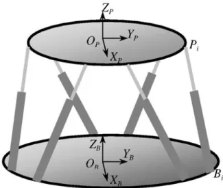
platform [1], as shown in Fig. 1, is a mechanical structure which has an upper platform and a lower base platform connected by six variable length links. When the length of each link is controlled properly, the upper platform is
capable of performing six degree-of-freedom motion within its working space. There are many research topics concerning this mechanical structure, including its construction, singular points and working space determination, forward and inverse kinematic problem solution, dynamic forces computation, motion control, and practical applications [2-12]. Here, we use the hy-draulic Stewart platform and its control system reported in [11] and [12] as the basic apparatus to develop a land vehicle driving simulator.
In addition to the motion generation device, a visual system is the other essential component in a driving simulator. It is needed not only because a virtual environment must be created in which the pilot of the simulated vehicle can drive around, but also because visual cues can greatly enhance the motion sensation of the pilot. Fortunately, computer graphics technologies are quite mature today, and many tools can be utilized to help build a reasonably good yet economical visual system. Foley, et al. [13] provided complete coverage of computer graphics theory, including topics such as appli-cation development, geometric transformation, model construction, devices, interactive skills, and the use of relevant software packages. Trujillo [14] discussed the background and use of the software Direct3D, a com-ponent of Microsoft DirectX. With the aid of this software, we have developed a visual system for our simulator, which creates animation scenes of the environment and shows them on a large screen in front of the pilot through an LCD projector. The scenes are designed to be synchronized with the pilot’s steering signals and the platform’s motion.
Below, we present the development details of the two main subsystems: the Stewart platform-based motion component and the computer graphics-based visual component. First, we define our symbols and conventions for three-dimensional coordinate frames in Section II, which will be used throughout the paper. Then, we briefly introduce the inverse kinematics of the Stewart platform in Section III and derive formulas for link lengths that will be needed to provide the specific upper platform position and orientation needed in the process of motion simulation. In Section IV, a simplified vehicle dynamic model is described, which mainly considers the influence of the vehicle suspension system. Based on this model, the motion of the pilot inside the vehicle is analyzed in Section V, and the part that the pilot is supposed to feel is extracted by means of a classical washout algorithm explained in Section VI, which generates the motion commands for the Stewart platform. After introducing the motion subsystem, we introduce in Section VII the visual component, which in cludes a big screen, an LCD projector, and a computer with an appropriate algorithm for generating suitable graphics. Finally, in Section VIII, we use a picture and a block diagram to present our experimental setup, and
give some experimental results obtained using the inte-grated system. Conclusions are given in Section IX.
II. RELATED COORDINATE FRAMES
First, we will define three right-hand orthogonal coordinate frames, FI, FC, and FV, needed to discuss the vehicle dynamics. For f = I, C, and V, let Xf, Yf, and Zf be the three principle axes of Ff with unit vectors If, Jf, and
Kf, respectively. The inertial frame FI is land-fixed, and
its z-axis is against the direction of gravity. The origin and the other two axes of FI are on flat ground on which the land vehicle moves. We assume that, initially, the vehicle is at rest and pointed toward the positive direction of XI. The origin of the vehicle frame FC is attached to the mass center of the vehicle, with its XC –YC plane always parallel to the XI –YI plane. The relation between FC and FI is a translation equal to the displacement of the vehicle’s center of mass, plus a rotation of angle θz about the ZC axis, depending on the yaw motion of the vehicle, so that the positive direction of XC keeps to be the vehicle moving forwards. The rotation matrix from FC to FI is, thus, given by RC I = Rz,θz= cz – sz 0 sz cz 0 0 0 1 , (1)
where cz and sz denote cos θz and sin θz, respectively. Similar notations will be used in the following. The origin of the coordinate frame FV is the same as that of FC, but its
XV and YV axes coincide with the forward longitudinal
and lateral body axes of the vehicle, respectively. More precisely, FV can be obtained by rotating FC by an angle θx about the XC axis, followed by rotating it by an angle θy about the YC axis, depending on the roll and pitch motion of the vehicle body, respectively. Obviously, the rotation matrix from FV to FC is RV C = Ry,θy⋅Rx,θx= cy 0 sy 0 1 0 – sy 0 cy ⋅ 1 0 0 0 cx – sx 0 sx cx = cy sxsy cxsy 0 cx – sx – sy sxcy cxcy , (2)
and the rotation matrix from FV to FI is RV I = RC I ⋅ RV C = cz – sz 0 sz cz 0 0 0 1 ⋅ cy sxsy cxsy 0 cx – sx – sy sxcy cxcy
=
cycz sxsycz – cxsz cxsycz + sxsz cysz sxsysz + cxcz cxsysz – sxcz
– sy sxcy cxcy
.
(3) In the sections that follow, we shall assume that with respect to FI, that FV has an angular velocity
ωIV=θxIC+θyJC+θzKC. (4)
At any fixed point A inside the vehicle body, we can further define a vehicle-fixed frame FA by trans-lating the origin of FV to the point A. This frame will be useful when we analyze the specific forces acting on the pilot and compute the pilot’s rotational velocity.
Finally, we need to mention two coordinate frames pertaining to the Stewart platform. In Fig.1, the base frame FB and the platform frame FP are defined with their origins located at the center of the base and the upper platform of the structure, respectively. The X-Y planes of the two frames coincide with the base and upper platform planes, respectively.
III. INVERSE KINEMATICS OF THE STEWART PLATFORM
The inverse kinematics problem for the Stewart platform is to determine link lengths given the relative translation and rotation of the upper platform with respect to the fixed base. Ignoring the translational difference for now, let the frame FP be obtained by rotating FB by an angle γ about the XB axis, followed by rotating it by an angle β about the YB axis, followed by rotating it by an angle α about the ZB axis. The rotation matrix from FP to FB is given by
RP B = Rz,α⋅Ry,β⋅Rx,γ = cαcβ cαsβsγ– sαcγ cαsβcγ+ sαsγ sαcβ sαsβsγ+ cαcγ sαsβcγ– cαsγ – sβ cβsγ cβcγ . (5)
Suppose the position vector from OB to OP, OBOP, has the following coordinate vector in the frame FB:
OBOPB = [x y z]T (6)
Note that, here, we adopt the convention of using a superscript after a vector to represent its coordinate vector in a certain coordinate frame. This convention will also be followed below, except for the superscript T, which is reserved for the transpose of column and row
vectors. From Fig. 2, we have BiPi B = OBOPB + OPPiB – OBPiB = OBOP B + RPB ⋅ OPPi P – OBBi B , (7)
in which OPPiP and OBBiB are constant vectors determined by the physical dimensions of the structure. Hence, the length of the i-th link is
li = BiPi B
2 . (8)
Note that the right side of (8) is a nonlinear function of the position and attitude variables (x, y, z, α, β, γ) of the upper platform. In other words, given any position and attitude of the upper platform within its working space, we can use (8) to determine all six link lengths that are required. For the Stewart platform in a driving simulator, (x, y, z, α, β, γ) of the upper platform must follow the trajectory commands generated by the system and the pilot. Thus, (8) is the key equation for motion realization, as link length changes can be imple-mented by controlling the hydraulic cylinder links appropriately.
IV. VEHICLE DYNAMIC MODEL [15]
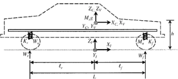
It is important to predict the vehicle dynamic re-sponses to the pilot’s inputs in an interactive driving simulator. In this section, we will introduce a simplified vehicle dynamic model, which considers mainly the dy-namic characteristics of the vehicle suspension system. For simplicity, all other sources of dynamic forces, such as engine vibration, structural flexibility, transmission ac-tions etc., are ignored. Consider the vehicle at rest on the
XI-YI plane as shown in Fig. 3.
When the vehicle is not moving, the static forces exerted by the ground on the front and rear wheels are
Wf= Mug + Msg r L , (9) Wr= Mug + Msg f L , (10)
respectively, where Ms is the mass of the vehicle body,
Mu is the mass of two suspension systems and wheels, g is
the gravitational acceleration, and f, r and L are
lengths shown in Fig. 3.
When the vehicle has forward acceleration ax at time t, we can take moments about points E1 and E2 in Fig. 4 to obtain the normal reaction forces on the front and rear wheels as Wf= Mug + Msg r L – Msax(h + sz) L , (11) Mr= Mug + Msg f L + Msax(h + sz) L , (12)
respectively, where h is the height of the vehicle’s center of mass when it is at rest, as shown in Fig. 3, and
sz is the shift of the vehicle’s center of mass along the
positive direction of ZC at time t. From (9)-(12), we know that the deflection of front and rear suspension is, respectively, ∆f= Msax(h + sz) LKf , (13) ∆r= Msax(h + sz) LKr , (14)
where Kf and Kr are the stiffness coefficients of the front and rear suspension systems, respectively. At the next instant t + ∆t, where 0 < ∆t << 1, the shift of the vehicle’s center of mass due to pitching of the vehicle body is
sz1= r
L∆f– f
L∆r, (15)
and the rotation angle of FV along the YC axis with respect to FC is
θy= – ∆f+∆r
L . (16)
For the lateral motion of the vehicle, consider Fig. 5. When the vehicle is not moving, the static forces ex-erted by the ground on the left and right wheels are, respectively, Wl= Mug + Msg drt D , (17) Wrt= Mug + Msg dl D , (18)
where drt, dl, and D are shown in Fig. 5. Suppose the vehicle has a velocity vx in the positive direction of XC and an angular velocity θz in the positive direction of ZC;
then, the centripetal acceleration is
ay=
vx 2
ρ = vxθz. (19)
Via similar derivation for the longitudinal case, we can obtain relative quantities at time t as
Wl= Mug + Msg drt D – Msay(h + sz) D , (20) Wrt= Mug + Msg dl D + Msay(h + sz) D , (21) ∆l= Msay(h + sz) DKl , (22) ∆rt= Msay(h + sz) DKrt . (23)
Consequently, we can determine the shift of the mass center at time t + ∆t due to the rolling of the vehicle body as sz2= drt D∆l– dl D∆rt (24)
Fig. 3. Side view of the vehicle at rest on the XI-XI plane.
θy
and the rotation angle of FV along the axis XC with respect to FC as
θx= ∆l+∆rt
D . (25)
Thus, at time t + ∆t, the total shift of the mass center is
sz = sz1 + sz2. (26)
V. PILOT MOTION ANALYSIS
In this section, we will analyze the motion of a fixed point A inside the vehicle body. In our simulator, this point will be the center of the pilot’s seat in the simulated vehicle, so we shall be able to describe the motion that the pilot will experience in appropriate frames. Let rVA be the
position vector from the origin of FV to point A; thus,
rVAV is a constant vector. Coordinate transformation gives rVA V = RIV⋅rVA I . (27) Hence, rVA V = RI V⋅ rVA I + RI V ⋅rVA I = 0 . (28) Symmetrically, we have rVA I = RI V⋅ rVA V + RV I ⋅rVA V = RV I ⋅ rVA V . (29)
According to the kinematics of non-inertial frames, we also have rVA I =ΩIV I ⋅ rVA V , (30) where ΩIV I = 0 –ωIV3 I ω IV2 I ωIV3I 0 –ωIV1I –ωIV2 I ω IV1 I 0 (31)
is skew-symmetric and [ω IV1I ωIV2I ωIV3I ] T
= ωIV
I
from (4). Based on (29) and (30), we see that
RV I ⋅rVA V =ΩIV I ⋅ rVA I =ΩIV I ⋅ RV I ⋅ rVA V . (32) Since rVA V
is arbitrary, it can be concluded that RV I =ΩIV I ⋅ RV I , (33) ΩIV I = RV I ⋅RI V . (34)
Now, if we treat FV as the fixed frame and FI as the rotating one with angular velocity –ωIV, we get
RI V ⋅rVA I = –ΩIV V ⋅ rVA V = –ΩIV V ⋅ RI V⋅ rVA I , (35) RI V = –ΩIV V ⋅ RI V . (36)
The orthogonality of FI and FV implies that RV I = (RI V )T= (RI V )– 1, (37) RV I = (RI V )T. (38)
Substitution of (36), (37), and (38) into (34) yields ΩIV I = (RI V )T⋅RI V = ( –ΩIV V⋅ RI V )T⋅RI V = RV I ⋅ Ω IV V ⋅ RI V , (39) which in turn can be substituted into (33) to produce
RV I = (RV I ⋅ Ω IV V⋅ RI V )⋅RV I = RV I ⋅ Ω IV V . (40) θz
Fig. 6. The vehicle turning right. Fig. 5. Rear view of the vehicle at rest.
From (29), (33), and (39), we get rVA I =ΩIV I ⋅ rVA I = (RV I ⋅ Ω IV V ⋅ RI V )⋅rVA I , (41)
which can be simplified as
RIV⋅ rVAI =ΩIVV ⋅rVAV . (42) The position vector rIA pointing from the origin of
frame FI to fixed point A can be expressed as the sum rIA I = rIV I + rVA I , (43)
where rIV is the position vector pointing from the origin
of frame FI to the origin of frame FV. If the vehicle has both translation and rotation motions in frame FI, then the first and second order time derivatives of the position vector rIA expressed in FI are, respectively,
rIA I = rIV I + RV I ⋅ Ω IV V ⋅ rVA V , (44) rIA I = rIV I + RV I (ΩIV V ⋅rVA V +ΩIV V⋅ Ω IV V⋅ rVA V ) , (45)
where (37), (40), and (42) are used to compute these derivatives. By taking RVI on (45) to the left side of the equation, (45) can also be used to express the second derivative of rIA in FV: RI V⋅ rIA I = RI V⋅ rIV I + (ΩIV V +ΩIV V⋅ Ω IV V )⋅ rVA V ) , (46)
where the first term on the right side can be changed to RI V⋅ rIV I = rIV V +ΩIV V⋅ rIV V (47) by taking the derivatives of both sides of the equation
rIVI = RVI ⋅rIVV (48)
and using (40).
For our simulator development problem, we can use (46) and (47) as well as (50) and(51) given in the next Section to compute the specific force and angular velocity on point A, the pilot’s seat. Note that the right hand sides of (46) and (47) are the vehicle angular and transla-tional velocities ΩIV
V
and rIV V
and the acceleration ΩIV V
and rIV V
represented in frame FV. These quantities can be easily determined from the information provided by the vehicle dynamic model introduced in Section IV.
VI. THE CLASSICAL WASHOUT ALGORITHM
To generate the sensation of motion for pilots driv-ing a simulator, a standard approach is to compute the specific force [16] acting on the pilot in the vehicle, which is defined as the nongravitational force per unit mass. Suppose from the vehicle dynamic model and the method described in Section V, we know that at a certain instant, the acceleration of the center of the pilot’s seat is a . Then the specific force acting on the pilot is
f ≡ a – g . (49)
Clearly, due to the motion capability and working space constraints, the Stewart platform can not re-create the specific force faithfully in the entire operational process. Thus, some adjustments are necessary so that only the part that can be sensed by the pilot is re-created. The principle human sensing organs for rotation motion and the specific force are the semicircular canals and otolith, respectively. The mathematical response models for the semicircular canals and otolith are shown in Fig. 7 and Fig. 8, and are active within the frequency region of 0.2 –10 rad/sec and 0.2 – 2 rad/sec, respectively. Exploiting the threshold and band-pass properties of the human motion sensation, the washout algorithms sug-gests how we can create a sensation of motion by per-forming translation and rotation of certain frequency bands only, and by replacing the sustained linear trans-lation with a tilt motion.
Consider the seat center point A on which the pilot sits. Because FA is merely a translation of FV, the specific force acting on point A has the same representation in both frames: fA A = fA V = RI V⋅ rIA I – RI V⋅ gI, (50)
and the angular velocity of point A with respect to FI is equal to that of the vehicle’s center of mass, i.e.,
ω δ
δTH
∆ Tas ωˆ
TLs
(TLs+1)(Tss+1) Tas + 1
Fig. 7. Mathematical response model of the semicircular canals [17,18].
f d dTH D (τ fˆ as+1) K (τLs+1)(τas+1)
ΩIA A =ΩIA V =ΩIV V . (51)
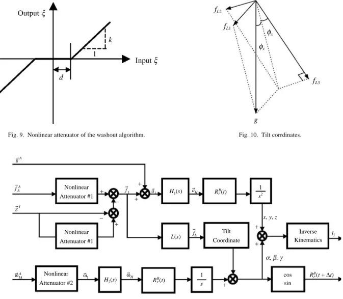
Note that the second equality in (50) comes from the results derived in Section V. To extract from (50) and (51) the parts that both need to and can be implemented on the Stewart platform, the classical washout algorithm [9,18] shown in Fig. 11 employs three functions. First of all, it generates platform translational motion commands x, y, and z by putting fAA through a nonlinear attenuator of the characteristics shown in Fig. 9 and a filter H1(s). The nonlinear attenuator is used to simulate the threshold effect of human sensation and to scale the amplitudes of the motion commands. The filter is used to eliminate the low frequency content of the motion commands to which the pilot is not sensitive. Secondly, it generates some of the platform rotational motion commands α, β, and γ by putting ωIA
A
from ΩIA A
in (51) through a nonlinear attenuator and a filter H2(s). Thirdly, it generates the remaining platform rotational motion commands. The purpose here is to implement the sustained linear
trans-Output ξ
Input ξ k
1 d
Fig. 9. Nonlinear attenuator of the washout algorithm.
gA ➞ fAA ➞ gI ➞ ω➞A IA ω ➞ 1 ω ➞ H f1 ➞ a➞1 a➞H fL ➞ Nonlinear Attenuator #1 Nonlinear Attenuator #1 Nonlinear Attenuator #2 H2(s) RP (t) B 1 s cos sin RP (t + ∆t) B + + + + + + + + − − L(s) Tilt Coordinate x, y, z Inverse Kinematics li 1 s2 RP (t) B H1(s) α, β, γ
Fig. 11. Classical washout algorithm.
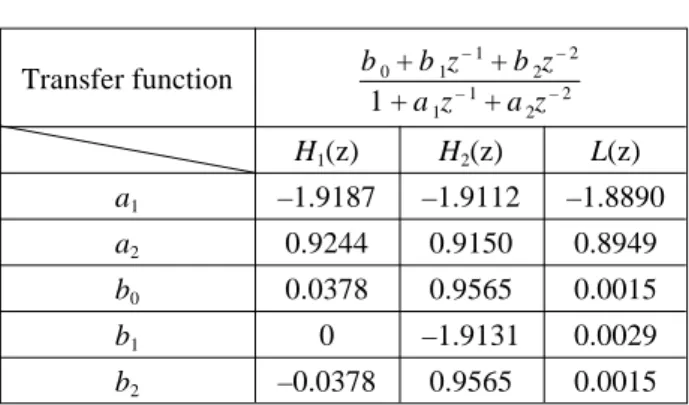
Fig. 10. Tilt corrdinates.
fL2 fL1 g fL3 φx φx
lational acceleration by means of tilt-coordinates shown in Fig. 10, where the relative tilt angles φ = [φx φy φz]T are φx= tan – 1 (fL2 fL3 ) , (52) φy= – tan ( fL1 fL3⋅cos (φx)) , (53) φz = 0, (54) and fL T = [fL1 fL2 fL3]T is obtained by putting fA A through a nonlinear attenuator in series with a low-pass filter L(s). Obviously, fL
T
is the specific driving force for the sensible part of the sustained linear translational acceleration, and if we tilt the upper platform with angles φx and φy around the axes XP and YP, respec-tively, then the gravity force will produce the first two
components of fL T
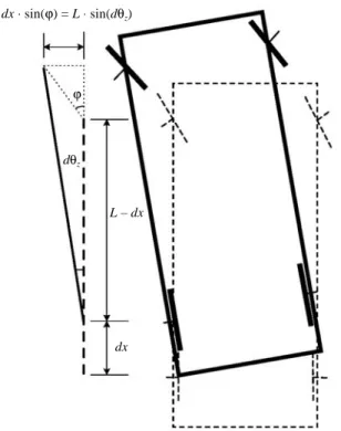
for us. The related parameters of the filters and nonlinear attenuators are listed in Tables 1, 2 and 3, respectively, in which the transfer functions of the filters are expressed by the z-transform because they need to be implemented by the digital computer.
VII. VISUAL SYSTEM
The visual system is needed not only to create a virtual environment for the pilot of the simulated vehicle to drive around in, but also to produce visual cues which greatly reinforce the sensation of motion experienced by the pilot. For our system, the image generation software was developed using the graphics tool package Direct3D on the operating system Windows 95. The environmental scenes, such as trees, road, and road signs, were con-structed using the method of texture mapping [13,14], as shown in Fig. 12. A typical scene like that shown Fig. 13, is displayed on a large screen in front of the pilot using an LCD projector. When the pilot inputs steering signals into the simulator through a joystick, we decide what the pilot should see by computing the position and orientation of the view port marked in front of the vehicle as shown in Fig. 12. In our system, two computers are
employed. The master computer receives/transforms commands, determines the view port, generates images in real time, and passes the transformed commands to the other computer, the slave computer, for the vehicle dynamics, utilizing the washout algorithm, and control-ling the Stewart platform.
Here, we will briefly describe how the position and orientation of the view port are computed. In response to steering signals, which are the axial acceleration ax and the front wheel turn angle ϕ, the master computer first determines the yawing velocity of the vehicle based on the relation given in Fig. 14, where L is defined in Fig. 3, dx is an infinitesimal translational displacement, dθz is an infinitesimal yaw angle, and
dx ⋅ sin(ϕ) = L ⋅ sin(dθz) ≈ L ⋅ dθz. (55) An infinitesimal time dt is divided on both sides to obtain dx dt ⋅sin (ϕ) = L⋅ dθz dt (56) or ωIC3 C =sin (ϕ) L ⋅vIC1 C , (57)
Table 1. Parameters of the filters.
Transfer function b0+ b1z – 1 + b2z – 2 1 + a1z – 1 + a2z – 2 H1(z) H2(z) L(z) a1 –1.9187 –1.9112 –1.8890 a2 0.9244 0.9150 0.8949 b0 0.0378 0.9565 0.0015 b1 0 –1.9131 0.0029 b2 –0.0378 0.9565 0.0015
Table 2. Parameters of nonlinear attenuator #1.
Surge Sway Heave
( x-axis ) ( y-axis ) ( z-axis)
Threshold value d
0.17 0.17 0.28
(m/sec2 )
Amplitude ratio k 0.4 0.4 0.4
Table 3. Parameters of nonlinear attenuator #2.
Roll Pitch Yaw
( x-axis ) ( y-axis ) ( z-axis)
Threshold value d
3.0 3.6 2.6
(deg/sec)
Amplitude ratio k 0.7 0.7 0.7
Fig. 12. Scene construction.
where ωIC3
C is the angular velocity of the vehicle about the
axis ZC, and vIC1 C
is the axial velocity of the vehicle. Note that vIC1
C
can be obtained by integrating the axial ac-celeration ax, which is the first component of aICC, i.e., aIC1
C . Clearly,
ωIC3C and vIC1
C together are sufficient to
define the position of the view port. As to the orientation of the view port, we use a simplified scheme to speed up the computation and graphics display. In Direct3D, every object in the scene belongs to some frame, and the view port is no exception. Also, a frame may be the “child” frame of some “parent” frame, which in turn may be the “child” frame of some other “parent” frame and, eventually of the “root” frame. We describe the transla-tional and yawing motion of the view port using a frame Z, which is the “child” frame of the “root” frame. Then, we describe the pitching motion of the view port using a frame Y, which is the “child” frame of the frame Z. Finally, we describe the rolling motion of the view port using a frame X, which is the “child” frame of the frame Y. Figure 15 shows the frame structure of the view port except that, actually, frames X, Y, and Z have the same origin. They are separated in Fig. 15 to facilitate presentation. For the view port, the pitching angle θy is the rotation angle of the Y-axis of the frame Y and is largely proportional to the axial acceleration aIC1
C
ac-cording to (13), (14), and (16). Therefore, θy=σy⋅aIC1
C
(58) where σy is a constant. Similarly, the rolling angle θx is the rotation angle of the X-axis of the frame X and is
largely proportional to the centripetal acceleration determined in (19) according to (22), (23), and (25). Therefore,
θx=σx⋅vIC1 C ⋅ω
IC3
C , (59)
where σx is a constant. Lastly, the yawing angle θz is the rotation angle of the Z-axis of the frame Z and can be obtained by integrating ωIC3
C .
VIII. EXPERIMENTAL RESULTS
Figure 16 shows the driving simulator assembled in the Advanced Control Laboratory of the Department of Electrical Engineering, National Taiwan University. The block diagram of its system configuration is shown in Fig. 17. In the system, the master computer generates
dx ⋅ sin(ϕ) = L ⋅ sin(dθz)
ϕ
dθz
dx L – dx
Fig. 14. Yawing velocity of the vehicle.
ax ωx az ωz ay ωy
Fig. 15. Frame structure of the view port.
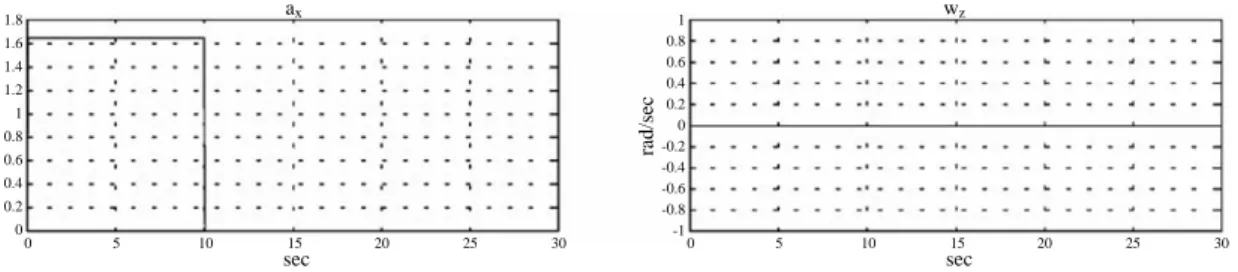
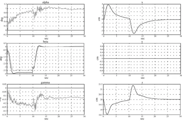
vehicle to accelerate constantly for 10 seconds without making any turns, and to cruise with zero acceleration afterwards. The resulting command signals for the plat-form orientation and position are the dark lines in each diagram in Fig. 19. Apparently, these command signals are correct, as the commands for α, γ, and y are all zero, and the commands for β, x and z reflect the motion that the pilot would experience at the beginning and end of a constant translational acceleration. Figure 19 also in-cludes the orientation responses (light lines) for α, β, and
γ of the platform measured by gyroscopes. These
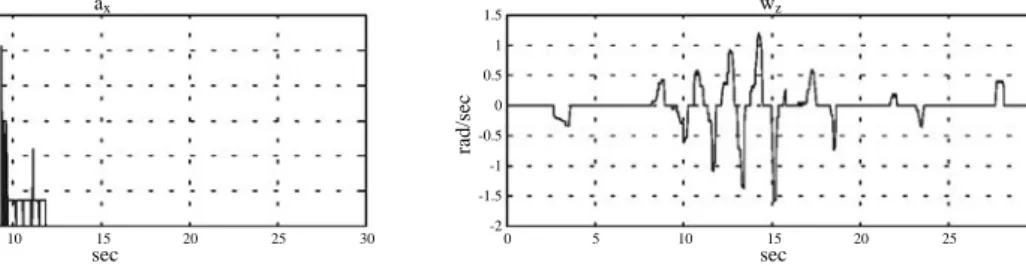
re-sponses contain some small tracking errors, which may be due to the bias of the gyroscope and to coupling between different degrees of freedom of platform motion. The second experiment was similar to the first one except that this time the simulated vehicle was required to make a turn while accelerating forwards. The steering signals are shown in Fig. 20. Note that it is the yawing velocity ωIC3C that is shown, not the front wheel turn angle ϕ received from the joystick. Again, we see that the resulting command signals for the platform orientation and position represented by the dark lines in Fig. 21 are reasonable, and that the orientation responses (light lines) measured by the gyroscope contain only small tracking errors. Finally, in the third experiment, a pilot tested the platform by steering it using the joystick and produced the steering commands displayed in Fig. 22. It is worth noting that even with these almost random inputs, the platform respondsed quite well, as the gyro-scopic outputs in Fig. 23 show. More detained results of these experiments can be found in [19].
IX. CONCLUSION
We have constructed a driving simulator by integrat-ing a realistic vehicle dynamic model and virtual reality technologies. The system has been tested thoroughly, and the performance has been found to be quite satisfactory. A video clip showing operation of the simulator and its components can be viewed at the Web site http://acl.ee. ntu.edu.tw. For more complex vehicles such as ships and aircraft, it will be possible to use the same approach to build simulators. More complex factors, such as road roughness, air resistance etc., will be introduced into our system in the future.
Joystick Input Pilot PCL-726 PCL-813 PCL-816
Gyro PlatformStewart LVDT Proportional Valve LCD Projector Display Area 150cm×100cm Pentium 200 Computer Graphic Generator (Master Computer)
Pentium Pro 180 Vehicle dynamics computation Stewart Platform Controller (Slave Computer)
Motion Cue
Visual Cue
16-bit A/D Converter 12-bit A/D Converter 12-bit D/A Converter
Fig. 17. Block diagram of the driving simulator.
1.8 1.6 1.4 1.2 1 0.8 0.6 0.4 0.2 0 1 0.8 0.6 0.4 0.2 0 -0.2 -0.4 -0.6 -0.8 -1 ax wz rad/sec m/s *s 0 5 10 15 20 25 30 sec 0 5 10 sec15 20 25 30
Fig. 18. Steering commands.
images at a rate of 25 pictures per second while the slave computer controls the motion of the Stewart platform based on the vehicle model at a rate of 400 Hz. This method of computational load sharing successfully satis-fies the real time operational requirements of the system. Also, because the steering commands received from the pilot are received by the master computer and used for signal processing, and are then passed to the slave com-puter which controls the motion part, visual cues and motion cues are well synchronized. Besides the computer part of the system, the mechanical part also plays an important role. As we mentioned above, the controller is based on the results reported in [11] and [12], where only LVDTs are meaning unclear feedback link lengths. Here, we add gyroscopes to record the real time orientation responses of the platform but do not feed the signals back to the controller, thus avoiding the bias effect of the gyroscopes. Use of the hydraulic Stewart platform en-ables us to carry heavy loads, such as human pilots, but also restricts the operational speed, compared with those of Stewart platforms driven by electric motors. However, the response time of the hydraulic actuators and controller adopted here is fast enough for this application project, as the test results to be presented below show.
Here, we will present three groups of experimental results obtained using this setup. In the first experiment, without putting a pilot on the platform, we let the master computer itself generate a set of steering signals shown in Fig. 18. These command signals asked the simulated
1.8 1.6 1.4 1.2 1 0.8 0.6 0.4 0.2 0 1.6 1.4 1.2 1 0.8 0.6 0.4 0.2 0 ax wz rad/sec m/s *s 0 5 10 15 20 25 30 sec 0 5 10 sec15 20 25 30
Fig. 20. Steering commands.
1.2 1 0.8 0.6 0.4 0.2 0 -0.2 4 3 2 1 0 -1 -2 -3 -4 alpha x cm de g 0 5 10 15 20 25 30 sec 0 5 10 sec15 20 25 30 0.5 0 -0.5 -1 -1.5 -2 -2.5 -3 -3.5 -4 1 0.8 0.6 0.4 0.2 0 -0.2 -0.4 -0.6 -0.8 -1 beta y cm de g 0 5 10 15 20 25 30 sec 0 5 10 sec15 20 25 30 0.05 0 -0.05 -0.1 -0.15 -0.2 -0.25 -0.3 -0.35 21.5 21 20.5 20 19.5 19 18.5 gamma z cm de g 0 5 10 15 20 25 30 sec 0 5 10 sec15 20 25 30
Fig. 19. Platform orientation/position commands and orientation responses.
REFERENCES
1. Stewart, D., “A Platform with Six Degrees of Freedom,” Proc. Inst. Mech. Eng., Vol. 180, Part 1, No. 5, pp. 371-386 (1965).
2. Yang, D.C.H. and T.W. Lee, “Feasibility Study of a Platform Type of Robotic Manipulators from a Kine-matic Viewpoint,” J. Mech., Transm. Autom. Design, Vol. 106, No. 1, pp. 191-198 (1984).
3. Fichter, E.F., “A Stewart Platform Based Manipulator: General Theory and Practical Construction,” Int. J. Rob. Res., Vol. 5, No. 2, pp. 157-182 (1986). 4. Do, W.Q.D. and D.C.H. Yang, “Inverse Dynamic
Analysis and Simulation of a Platform Type of Robot, ” J. Rob. Syst., Vol. 5, No. 3, pp. 209-227 (1988). 5. Liu, K., “Modeling and Control of a Stewart Platform
Manipulator,” Amer. Soc. Mech. Eng., Dyn. Syst. Contr. Division, Vol. 33, No. 1, pp. 83-89 (1991). 6. Liu, K., J.M. Fitzgerald and F.L. Lewis, “Kinematic
Analysis of a Stewart Platform Manipulator,” IEEE Trans. Ind. Electron., Vol. 40, No. 2, pp. 282-293 (1993).
7. Reid, L.D., “Motion Algorithm for Large-Displace-ment Driving Simulator,” Transpo. Res. Record, No. 1403, pp. 98-106 (1993).
8. Salcudean, S.E., P.A. Drexel, D. Ben-Dov, A.J. Tay-lor and P.D. Lawrence, “A Six Degree-of-Freedom, Hydraulic, One Person Motion Simulator,” Proc. IEEE Int. Conf. Rob. Autom., San Diego, CA, USA, pp. 2437-2443 (1994).
9. Grant, P.R. and L.D. Reid, “Motion Washout Filter Tuning: Rules and Requirements,” J. Aircraft, Vol. 34, No. 2, pp. 145-151 (1997).
10. Pouliot, N.A. and C.M. Gosselin, “Motion Simulator Capabilities of Three-Degree-of-Freedom Flight Simulators,” J. Aircraft, Vol. 35, No. 1, pp. 9-17 (1998).
Control of a Hydraulic Stewart Platform, Part I: Kine-matics and Dynamics Analysis,” J. Contr. Syst. Technol., Vol.6, No.3, pp. 177-184 (1998).
12. Wen, C., C.-C. Hsu and I-K. Fong, “Modeling and Control of a Hydraulic Stewart Platform, Part II: Modeling and Control of the Hydraulic Links,” J. Contr. Syst. Technol., Vol.6, No.3, pp.185-192 (1998). 13. Foley, J.D., A. van Dam, S.K. Feiner, J.F. Hughes and R.L. Phillips, Introduction to Computer Graphics, Addison Wesley, New York (1994).
14. Trujillo, S., Direct 3D Programming, The Coriolis Group, Scottsdale (1996).
15. Dukkipati, R.V., M.O.M. Osman and S.S. Vallurupalli, “Adaptive Active Suspension to Attain Optimal Per-formance and Maintain Static Equilibrium Level,”
2 1.5 1 0.5 0 -0.5 -1 4 3 2 1 0 -1 -2 -3 -4 alpha x cm de g 0 5 10 15 20 25 30 sec 0 5 10 sec15 20 25 30 0.5 0 -0.5 -1 -1.5 -2 -2.5 -3 -3.5 -4 4 3 2 1 0 -1 -2 -3 -4 beta y cm de g 0 5 10 15 20 25 30 sec 0 5 10 sec15 20 25 30 4.5 4 3.5 3 2.5 2 1.5 1 0.5 0 -0.5 23 22.5 22 21.5 21 20.5 20 19.5 19 18.5 18 gamma z cm de g 0 5 10 15 20 25 30 sec 0 5 10 sec15 20 25 30
Fig. 21. Platform orientation/position commands and orientation responses.
Int. J. Vehicle Design, Vol. 14, No. 5, pp. 471-496 (1993).
16. Pitman, G.R., Inertial Guidance, John Wiley, New York (1962).
17. Zacharias, G.L., “Motion Cue Model for Pilot-Ve-hicle Analysis,” AMRL-TR-78-2 (1978).
18. Reid, L.D. and M.A. Nahon, “Flight Simulator Mo-tion-Base Drive Algorithms: Part 1 – Developing and Testing the Equations,” UTIAS Report No.296, CN ISSN 0082-5255 (1985).
19. Tseng, H.-L., “Implementation of a Driving Simula-tor Based on Stewart Platform and Computer Graph-ics Technologies,” Master Thesis (in Chinese), Insti-tute of Electrical Engineering, National Taiwan Uni-versity (1999). 3 2.5 2 1.5 1 0.5 0 1.5 1 0.5 0 -0.5 -1 -1.5 -2 ax wz rad/sec m/s *s 0 5 10 15 20 25 30 sec 0 5 10 sec15 20 25 30
Hung-Lung Tseng was born in 1971 in Taipei and received his M. Sc. from Nationa Taiwan University in electrical engineering in 1999. Be-fore receiving his M.S. degree, he held a research position in the industry. In the Institute of Electrical Engineering at NTU, he was a mem-ber of the control group, and his main research topics included motion/visual cue technologies for virtual reality systems as well as the construction of a vehicle driving simulator using a Stewart platform in the Advanced Con-trol Laboratory of the Institute. Currently, he works for the Nanya Technology Corporation as a Computer Integrated Manufacturing engineer. 1.8 1.6 1.4 1.2 1 0.8 0.6 0.4 0.2 0 -0.2 3 2 1 0 -1 -2 -3 alpha x cm de g 0 5 10 15 20 25 30 sec 0 5 10 sec15 20 25 30 1.5 1 0.5 0 -0.5 -1 -1.5 beta y cm 0 5 10 15 20 25 30 sec 0.5 0 -0.5 -1 -1.5 -2 -2.5 -3 -3.5 -4 de g 0 5 10 15 20 25 30 sec 1 0.8 0.6 0.4 0.2 0 -0.2 -0.4 -0.6 -0.8 21.5 21 20.5 20 19.5 19 18.5 18 17.5 17 gamma z cm de g 0 5 10 15 20 25 30 sec 0 5 10 sec15 20 25 30
Fig. 23. Platform orientation/position commands and orientation responses.
I-Kong Fong received his B. Sc. and Ph.D. degrees, both in electrical engineering, from National Taiwan University, Taipei, in 1981 and 1986, respectively. From 1984 to 1986 and from 1987 to 1993, respectively, he was an instructor and Associate Pro-fessor in the Department of Electrical Engineering, National Taiwan University. During 1986, he conducted research at the University of California, Davis, as a Research Associate. Since 1993, he has been a Professor in the Department of Electrical Engineering, National Taiwan University. Currently, his research inter-ests include robust control theory, flight control systems, dynamic optimization methods, and decentralized control systems.

![Fig. 7. Mathematical response model of the semicircular canals [17,18].](https://thumb-ap.123doks.com/thumbv2/9libinfo/8856084.243832/6.892.466.802.919.980/fig-mathematical-response-model-semicircular-canals.webp)