Abstract
This paper proposes an adaptive learning method for tracking targets across multiple cameras with disjoint views. Two visual cues are usually employed for tracking targets across cameras: spatio-temporal cue and appearance cue. To learn the relationships among cameras, traditional methods used batch-learning procedures or hand-labeled correspondence, which can work well only within a short period of time. In this paper, we propose an unsupervised method which learns both spatio-temporal relationships and appearance relationships adaptively and can be applied to long-term monitoring. Our method performs target tracking across multiple cameras while also considering the environment changes, such as sudden lighting changes. Also, we improve the estimation of spatio-temporal relationships by using the prior knowledge of camera network topology.
1. Introduction
Camera networks are extensively used in visual surveillance systems because they can monitor the activities of targets over a larger area. One of the major tasks of camera networks is to track targets across cameras. Several papers have previously discussed multi-camera tracking with overlapping field of views (FOVs), such as [1, 2, 13, 24]. However, in practice, it is hard to expect that the FOVs of cameras are always overlapping to each other. In this paper, we focus on solving the multi-camera tracking problem that the FOV of cameras are not necessarily overlapping.
There has been some notable works in tracking objects across non-overlapping cameras. Huang and Russell [9] first presented a probabilistic approach for object identification across two non-overlapping cameras, and then Pasula et al. [19] extended this approach for tracking through more than two sensors. Kettnaker and Zabih [12] employed a Bayesian formulation of the problem to reconstruct the paths of objects across multiple cameras, and transformed it into a linear-programming problem to
establish correspondence. Porikli and Divakaran [20] proposed a color calibration model estimating the optimal alignment function between the appearance histograms of the objects in different views, and then combined spatio-temporal and appearance cues to track objects. Javed et al. presented a system [10] that learned the camera network topology and path probabilities of objects using Parzen windows. They proposed an appearance model in [11], which learned the subspace of inter-camera brightness transfer functions for tracking. Dick and Brooks [6] employed a stochastic transition matrix to describe the observed pattern of people motion, which can be used within and between fields of view. In the training period, the observations are generated by a person carrying an easily identified marker. The methods mentioned above either assumed that the camera network topology and transition models are known, or fit them with hand-labeled correspondence or obvious markers. In practice, they are difficult to implement for real situations due to the complicated learning phase; in particular, when the environment changes frequently (such as lighting changes), the above scenarios will fail to work.
Makris et al. [15] proposed a method which does not require hand-labeled correspondence and automatically validate a camera network model using within-camera tracking data. This approach has been extended by Stauffer [22] and Tieu et al. [25] by providing a more rigorous definition of a transition based on statistical significance. Gilbert and Bowden [7] extended Makris’s approach to incorporate coarse-to-fine topology estimations, and further proposed an incremental learning method to model both the color variations and posterior probability distributions of the spatio-temporal links between cameras.
Tracking targets across multiple cameras with disjoint views is generally a correspondence problem dependent on two visual cues: spatio-temporal cue and appearance cue. To learn the spatio-temporal relationship, the methods [7, 15, 22, 25] learn it automatically. In [15, 22, 25], they used batch learning procedures, and estimated the entry/exit zones in advance. However, there are some limitations with their methods. First, how much training data is required in the batch-learning procedure remains unclear. Second, if the environment changes, the only solution is to reboot the
An Adaptive Learning Method for Target Tracking across Multiple Cameras
Kuan-Wen Chen
1Chih-Chuan Lai
2Yi-Ping
Hung
2,1,3Chu-Song Chen
3,2 1Dept. of Computer Science and Information Engineering, National Taiwan University, Taiwan
2
Graduate Institute of Networking and Multimedia, National Taiwan University, Taiwan
3Institute of Information Science, Academia Sinica, Taiwan
whole system since a batch-learning procedure was used. The method of [7] learned the spatio-temporal relationship incrementally, but the spatio-temporal links are block-based instead of entry/exit zone based, where the later can usually be learned from a single image efficiently. Furthermore, the paper did not show when to split the block, which is an important issue for real applications. The number of blocks may grow quickly although a coarse-to-fine estimation method was proposed.
The appearance relationships are also called the brightness transfer functions (BTFs), which transfer the color distribution from one camera to another. To our knowledge, the method proposed in [7] is the only one that learns it without hand-labeled correspondence. It seems adaptive to lighting changes due to the incremental learning procedure. However, the method needs much learning data, and so it is difficult to handle sudden lighting changes. For example, a lamp in a passage may be turned on, and then turn off after three hours. However, the time to learn the BTF is much more than three hours, and hence we will never obtain a correct BTF.
In this paper, we propose a new method that learns both spatio-temporal relationships and BTFs adaptively. To learn the spatio-temporal relationships, we introduce two improvements, the employments of prior knowledge of camera network topology and adaptive spatio-temporal relationships, which help track targets among multiple cameras with better performance. To learn BTFs, we present an unsupervised learning method. The required training data is much less than that in [7]. Our method is thus adaptive to handle sudden lighting changes – a situation usually happens in indoor environments, unavoidable for long-term monitoring, but has not been handled by previous methods to our knowledge.
2. Learning Spatio-Temporal Relationships
In this section, we first introduce the prior knowledge of camera network topology which improve the estimations of spatio-temporal relationships. Then, we present a method to learn the spatio-temporal relationships adaptively.2.1. Prior knowledge of camera network topology
Prior knowledge of camera network topology is prior information, which can be easily obtained manually in practical applications. It was never used in previous works, but it helps improve the learning of spatio-temporal relationships. The prior knowledge is as follows:
(1) Knowledge describing which pairs of cameras are adjacent.
(2) Knowledge describing whether the blind regions are closed or open, where the blind regions are those regions not monitored by any cameras. A blind region is closed if there are no entries and exits inside it;
otherwise it is open.
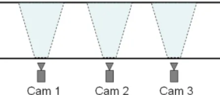
Advantages of employing prior knowledge of camera network topology are discussed as follows. First, the prior knowledge considerably decreases the computation complexity; we just need to learn the relationships between adjacent cameras. Second, they help remove the redundant links, which usually take much time to discover when we try to discover them automatically. As shown in Figure 1, there would be a redundant link produced between Cam 1 and Cam 3 for all of the automatically learning methods mentioned above. However, in real situations it is impossible to exit from Cam 1 and then enter Cam 3, without passing Cam 2. Third, there are some situations that can not be automatically learnt. For example, it is difficult to discover whether a blind region between cameras is closed or open, but this knowledge would help the non-overlapping camera network tracking. In particular, it is practically quite often that the blind regions are closed for indoor environments, such as buildings and parking garages.
Figure 1. A passage with three cameras and their fields of view.
2.2. An adaptive method for learning
spatio-temporal relationships
In our method, the spatio-temporal relationships are entry/exit zone based [15, 22, 25], and the learning procedures contain two phases: batch learning phase and adaptive learning phase.
In the batch learning phase, we estimate the entry/exit zones for each single image at first. We gather a lot of entry/exit points for each camera view with the results of single camera tracking. In each camera view, we model the entry/exit zones as a Gaussian Mixture Model (GMM) and use Expectation Maximization (EM) algorithm to estimate parameters of GMM [5, 14]. The number of clusters is determined automatically according to Bayesian Information Criterion (BIC).
After the estimations of entry/exit zones, the transition probability is learnt for each possible link according to the prior knowledge of camera network topology. Assume that there is a possible link between two entry/exit zones, zone a is in the view of camera A and zone b is in the view of camera B. Denote by pab(t) the transition probability that
someone moves from zone a to zone b at time t, and T is the maximum allowable reappearance period. The object i exits from the zone a with the time ti. The object j enters the zone
objects i and j, defined in our approach as the histogram intersection Sij =
∑
mh 1= min(Bih,Bjh), where m is the binnumber of the appearance color histogram, and Bih and Bjh
are the probabilities of the bin h in the histograms of objects i and j respectively. Then, the transition probability is calculated as: , 0 , 0 ) ( 1 ) (
∑∑
∀ ∀ ≥ < ∀ ⎪⎩ ⎪ ⎨ ⎧ − = = i j i j ij ab t T t otherwise t t t if S C t p (1) where∑
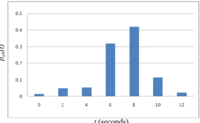
= = T t pab t C 0 () is a normalization term. An example of pab(t) is shown in Figure 2. After the transitionprobability estimation, we measure the noise floor level for each link. The noise floor level in our system is set as the double of the median value. If sufficient evidence has been accumulated and the maximum peak of the distribution exceeds the noise floor level, the possible link is set as a valid link between zones.
In the adaptive learning phase, we update the entry/exit zones and transition probability as time goes on. According to the definition of transition probability between zones, shown in Equation. 1, and learning it adaptively is simple.
Figure 2. An example of a transition probability distribution. There are some problems with the batch learnt entry/exit zones [15, 22, 25]. First, it is likely to misclassify two zones into one single zone when the two zones are close in the image, as shown in Figure 3(b). On the other hand, it could possibly divide a zone into several smaller zones. Second, the environment may change due to camera addition/removal. We may also lack the training data when there are no objects entering a room or passing some passages during the data-collection period of the batch learning phase. For solving the problem, we update the entry/exit zones by using on-line K-means approximation to update the mixture model [23] after the tracking correspondence being estimated. In addition, we propose some operators for learning zones adaptively: Zone Addition, Zone Merging, and Zone Split. The Zone Addition adds a Gaussian model with a slight weight for initialization into the GMM, and it is used when sufficient
evidence has been accumulated in a place. The Zone Merging merges two Gaussian models in GMM, which means two zones are seen as the same entry/exit zone. It is applied when two zones are near enough and found to have similar distributions and valid links to other zones. After each zone updating, we use Hotelling’s T-square test and W statistic test for testing the mean equality and covariance equality respectively [21], and then determine whether two zones are needed to be merged. When passing both tests, two zones are merged. The Zone Split is used for solving the problem, i.e. misclassify two zones into one single zone as shown in Figure 3. When a zone includes two valid links to different zones, it is split into two different zones. However, for lack of the information, it is hard to correctly initialize the parameters of the two zones. For the zone to be split, we generate a new Gaussian with the same covariance as the original one. Then we adjust the means of the two Gaussians along their principal axis in the opposite direction and reduce their mixture weightings by half assuming that they have an equal weighting. Due to the different spatio-temporal distributions, the two Gaussians will be adapted to isolated zones with time.
(a) (b)
Figure 3. An example of entry/exit zone estimation for Cam 3 in Figure 6. (a) the entry/exit zones, A, B, and C, after batch learning phase. (b) the entry/exit zones, A, B, C, and D, after adaptive learning phase. Note that zones C and D are very close. The zone C in (a) is split and adapted to zones C and D in (b) incrementally.
3. Learning Brightness Transfer Functions
In [7], the BTF is an m×m matrix, when the appearance is modeled as an m-bin histogram. Because the BTF is high dimensional and it is learnt without considering the correctness of each matching pair, learning it needs much data. The paper declares that the BTF would be refined as additional data is considered. However, this assumption is unsuitable for real environments where the light changes frequently. Javed et al. [11] showed that all BTFs from a given camera to another camera lie in a low dimensional subspace, but their method fitted them with hand-labeled correspondence. In this section, we propose an unsupervised learning method for a low dimensional subspace of BTFs by using the spatio-temporal information and Markov Chain Monte Carlo (MCMC) sampling. t (seconds) pab (t ) A B C C A B D
3.1. Brightness transfer functions
The appearance is modeled as a normalized histogram, because it is relatively robust to changes in object pose. Let fij be the BTF for every pair of observations Oi and Oj in the
training set, and assume that the percentage of image points in Oi with brightness less than or equal to Bi is equal to the
percentage of image points in Oj with brightness less than
or equal to Bj. If Hi and Hj are normalized cumulative
histograms respectively, then we have )) ( ( ) ( 1 i i j i ijB H H B f = − (2)
For learning the low dimensional subspace of BTFs, we use the probabilistic Principal Component Analysis PPCA [11]. Then, a d dimensional BTF, fij, can be written as
ω + + = ij ij Wy f f (3)
where y is a normally distributed q-dimensional subspace variable, q < d, and W is a d × q dimensional projection matrix.
ij
f is the mean of collection of BTFs, and ω is
isotropic Gaussian noise, i.e., ω ~ N(0, σ2I). Given that y
and ω are normally distributed, the distribution of fij is
given as ) , (f Z N fij= ij (4) Where Z = WWT+σ2I. More details can be found in [11, 26].
As shown in Figure 4, the reconstruction error, i.e. error of the transformed brightness histogram based on the reconstructed BTF, would decrease slowly if the number of data is larger than a bound. This means the BTF can be learnt with less data.
Figure. 4. The average reconstruction error decreases when the number of learning data increases. The Camera id is shown in Figure 6.
3.2. Criterion for BTF estimation
According to the discussion in [11], Javed et al. illustrated that when both the observations Oi and Oj belong
to the same object, the transformed histogram gives a much better match as compared to direct histogram matching. However, if the observations Oi and Oj belong to different
objects then the transformed histogram is reconstructed
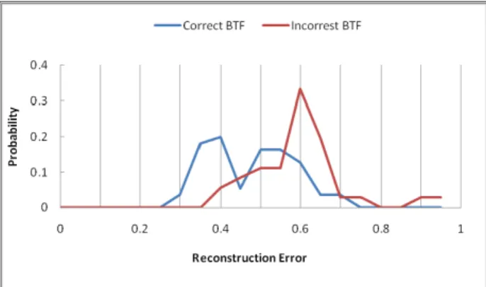
poorly, and the error either increases or does not change significantly. This is confirmed in our experiments. As shown in Figure 5, a correct BTF learnt by using correct correspondences would have a more diverse reconstruction error distribution and lower errors than the one learnt by using incorrect correspondences. Therefore, we propose a criterion p(π) for BTF estimation, where π is the sampled learning data set for BTF. We denote similarity(pairi) to be
the similarity score of the ith corresponding pair, which is calculated by (1-reconstruction_error(pairi)). Then, the
criterion is
(
( ))
)
( mean similarity pairi
p π = , (5)
for all i, if similarity(pairi)>Tc
where Tc is a threshold value, which is decided by Otsu’s
thresholding algorithm [18].
Figure 5. An example of the reconstruction error distribution estimated by testing the hand-labeled correspondencewith 50% matching accuracy.
3.3. Spatio-temporal information and MCMC
sampling
In this paper, the BTF is learnt without hand-labeled correspondence by sampling from the training data set and choosing the best BTF according to the criterion described in Section 3.2. However, it is not practical to sample all of the permutations directly, because the whole permutation-space is too large to search. For example, if there are n observations in both cameras, the number of matching permutations are n!, but the correct correspondences are at most n pairs.
Therefore, we use the spatio-temporal information to choose one possible solution from n! matching permutations. We get n pairs of target correspondences and their corresponding probability by using the spatio-temporal relationship. According to the experiments, the ratio of correct match is more than 60 percent by using the spatio-temporal cue only, which means that more than half of the n pairs are correctly matched. Then, we can sample k pairs, denoted by π, for learning the subspace of BTFs, where k (k < n) is the number of corresponding pairs
needed for learning. By sampling R times and k pairs per time, we choose the best one based on the criterion, Equation 5, to test the remainder data.
We sample by using Markov Chain Monte Carlo (MCMC) [4, 25] and use Metropolis-Hastings algorithm [8, 25] (see Algorithm 1). The initial sample π0 is based on the
corresponding probability. New samples π’ are obtained given the current one πr via a proposal distribution q(π’|πr),
where πr is the rth rounds of sampling results. We employ
four types of proposals for q(π’|πr). First, swap a pair, and
this swaps one of the k pairs chosen in the last time for one of the other (n−k) pairs. Second, jump, and this re-samples the whole k pairs. Third, add a pair, i.e., incrementing k by 1. Fourth, subtract a pair, i.e., subtracting k by 1. The third and fourth proposals are used for avoiding k being decided incorrectly. The new sample is accepted with a probability proportional to the relative likelihood of the new sample versus the current one. The likelihood is proportional to the criterion mentioned in Section 3.2. After executing the algorithm, the best sampling result recorded is chosen for learning the subspace of BTFs.
Algorithm 1. Metropolis-Hastings algorithm.
3.4. Adaptively learning BTF
It is always a problem that how many data is needed for learning a BTF in real applications, so we propose a method which updates the BTF adaptively. When gathering a constant number of data, we learn a BTF and then merge it with the old one. We use the method introduced in Sections 3.1-3.3 to learn the low dimensional subspace of BTF. We then merge two PPCAs by the method proposed by Nguyen and Smeulders [17]. In Figure 9, it shows that the reconstruction error decreases with more BTFs merged. Furthermore, it is adaptive to handling gradual lighting changes.
4. Target Tracking across Multiple Cameras
4.1. Problem formulation
Multi-Camera tracking with disjoint views seeks to establish correspondence between observations of objects across cameras. This is often termed as object “handover,” where one camera transfers a tracked object or person to another camera. The handover list is a set of observations having left from one camera view within the maximum allowable reappearance period or in the closed links. Suppose that a person E enters the view of one camera and denote this observation as OE, we could get from OE the
spatio-temporal cue st(OE) and the appearance cue app(OE).
The st(OE) includes the information of the arrival camera id,
location s(OE) and time t(OE). Then, the best corresponding
person with the observation Oh in the handover list is
selected. If the probability exceeds a threshold, we could decide that the newly arrival observation OE and the
observation Oh in the handover list are associated with the
same person. Otherwise, E is the new person arriving in the monitored environment. Denote the probability of the observation OE belonging to Oh in the handover list as
) ,
(E hOE Oh
p = ∣ . The most likely correspondence could be obtained as follows: )) , ( ( max arg E h H h O O h E p h s ∣ = = ∈ (6) where Hs is the handover list. Assume that the p(E=h) and
the observation pairs p(OE,Oh) are uniformly distributed,
and the spatio-temporal cue and appearance cue are independent. We take log likelihood and merge them by using a weight w, which is adaptive to the changes of environments. From Bayes Theorem, we have
)) ) ( ), ( ( ln ) 1 ( ) ) ( ), ( ( ln ( max arg )) ) ) ( ), ( ( ) ) ( ), ( ( (ln( max arg )) , | ( (ln max arg ) 1 ( h E O app O app p w h E O st O st p w h E O app O app p h E O st O st p O O h E p h h E h E H h w h E w h E H h h E H h s s s = × − + = × = = × = = = = ∈ − ∈ ∈ ∣ ∣ ∣ ∣ (7)
The p(app(OE),app(Oh)∣E=h)) is the probability of appearance similarity after color transformation by using the estimated BTF, which can be calculated as the histogram intersection SEh or Bhattacharyya coefficient [3].
Suppose that the entry/exit zones of OE and Oh are ZE and Zh
respectively, and pab(t) is the transition probability that
someone transits from zone a to zone b at time t. Then, we estimate
1. Initialize π0; r = 0. 2. loop
3. Sample π’ from q(.|π). 4. Sample U from U(0,1). 5. Let ⎟⎟ ⎠ ⎞ ⎜⎜ ⎝ ⎛ ′ ′ ′ = ′ ) | ( ) ( ) | ( ) ( , 1 min ) , ( r r r r q p q p π π π π π π π π α 6. if U ≦α(πr,π′) then 7. πr+1 = π’. 8. else 9. πr+1 =πj. 10. end if 11. r = r+1. 12. end loop
∑∑
∑∑
∀ ∀ ∀ ∀ = = = × = = = E h h E E h Z Z h h E E Z Z h h E E Z Z h E h E h E Z O s p Z O s p t p h E Z O s p h E Z O s p h E O t O t Z Z p h E O st O st p ) ) ( ( ) ) ( ( ) ( ) , ) ( ( ) , ) ( ( ) ) ( ), ( , , ( ) ) ( ), ( ( ∣ ∣ ∣ ∣ ∣ ∣ (8)wherepZEZh(t)is the transition probability distribution with t=t(OE)-t(Oh), and p(s(O⋅•)∣Z•) is the probability of the
observation O• entering or exiting from the zone Z , • which is GMM learned for the entry /exit zones. Note that, it considers all the entry/exit zones, and avoids classifying fault about adjacent zones.
4.2. Implementation
Initially, the prior knowledge of camera network topology is determined manually. Note that, in practical applications, this prior information can be easily obtained and the benefits are mentioned in Section 2.1. At bootup, the system collects observation data for a period of time, though this is not strictly necessary due to the adaptive learning procedure. Then, the entry/exit zones of each camera view are learnt first. Secondly, we learn the transition probability distribution of possible links. Finally, we learn the BTF for each pair of cameras, which depends on the spatio-temporal relationships, and treat each color channel separately.
When the system is processing, tracking targets across multiple cameras, as described in Section 4.1, is simultaneous with updating both the spatio-temporal relationships and appearance relationships. The transition probability distribution and entry/exit zones are updated for each arrival event. The BTF is learnt and merged after collecting a constant number of matching data.
4.3. Handling sudden lighting changes
The weight w, described in Section 4.1, indicates the confidence of learnt spatio-temporal relationship and BTF. It is adaptive to the changes of environments. To long-term monitoring, the changes of spatio-temporal relationships do not occur frequently. However, it usually occurs for appearance relationships, which are influenced by lighting changes. We have proposed an adaptive method to handle gradual lighting changes. Here, we use the weight w for handling sudden lighting changes, which occur regularly in indoor environments. In [16], Mittal and Huttenlocher proposed a method to detect sudden lighting changes in single camera view by taking a high normalized correlation and a high number of unmatched points. When detecting the event of sudden lighting change, we set the weight w to a higher value, which means that the spatio-temporal cue is more reliable than the appearance cue, and the BTF is
initialized as an identity matrix. It will decrease to half gradually with our adaptive learning procedure. Note that our method learns a BTF by using a few data only, and so it adapts to lighting changes soon.
5. Experimental Results
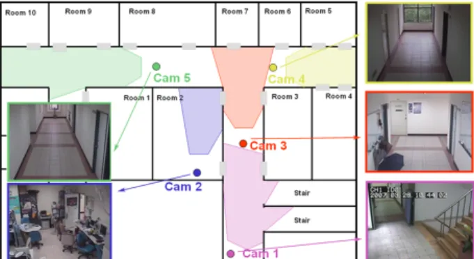
Our experimental environment is shown in Figure 6, and there are five cameras with disjoint views. We record for a 3-hour period. The manually specified camera network topology is shown in Figure 7.
Figure 6. The experimental environment includes five cameras. The colored circle means the position of camera, and the region with corresponding color is field of view of the camera.
Figure 7. The prior knowledge of camera network topology used in the experiment, given that all blind regions are closed. The camera id is shown in Figure 6.
5.1. Comparison
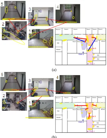
First, we compare our method with the method proposed by Makris et al. [15] for learning the spatio-temporal relationships. Figure 8.(a) shows the results by their method which is a batch learning method by using the whole 3-hour data. There are some valid links missed due to the lack of data, and it includes redundant valid links. Figure 8.(b) shows the results estimated by our method, and we use the data during the first hour for batch learning and the remaining data for learning adaptively. The correct valid links and entry/exit zones without clustering fault are learnt. The video sequence ( http://ivlab.csie.ntu.edu.tw /demodownload/LearnST.avi ) shows the adaptively learning process. We use varied lines to represent the strength of links, and the thick and red line means the valid links. It demonstrates that: (1) even lacking data when batch learning, the result is improved by adaptive learning
5 3 4
2
procedure, and (2) it overcomes the clustering fault of entry/exit zones incrementally.
(a)
(b)
Figure 8. The valid links and entry/exit zones estimated by using (a) Makris’s method, and (b) our method. The lower-right map shows the corresponding valid links and entry/exit zones. The red lines represent the correct valid links, and the blue lines are incorrect valid links estimated.
Second, we compare our method with the method proposed by Gilbert and Bowden [7] for learning the appearance relationships. The appearance is modeled as a 256-bin histogram in this experiment. Their BTF is therefore a 256×256 matrix learnt by using the incremental learning procedure. Our BTF is a learnt by adaptively learning method described in Section 3, with dimension q equal to 10. We test the camera pair of Cam 3 and Cam 4 and use the same correspondence determined by our spatio-temporal relationship, and compare the learning rate of BTF by calculating the average reconstruction error of 118 pairs of hand-labeled corresponding data. In the experiments, the period of passing 50 pairs of correspondences is about one and a half hours. As shown in Figure 9, our method has a faster learning rate, and their method never learns a stable BTF in the testing period. It demonstrates that our method learns well by using little number of data and can re-build the appearance relationship models soon after sudden lighting changes.
Figure 9. The reconstruction error with increasing number of passing correspondences for both Gilbert and Bowden’s method and our method.
5.2. Tracking results
The proposed system is trained for a 2-hour period, and evaluated by using unseen ground-truth of half an hour. The maximum allowable reappearance period T is set as 15 seconds, and appearance color histogram is 256-bin for each RGB color channels. The tracking accuracy is defined as the ratio of the number of objects tracked correctly to the total number of objects that passed through the scene, and is given in Table 1. We also compare the performance with the hand-labeled method, i.e. the entry/exit zones and the valid links between zones is determined manually and appearance histograms are matched directly (i.e. without transforming by BTF). It shows that our method has high tracking accuracy and considerable improvement in the following cases: (1) different lighting conditions between cameras, e.g. the pair of Cam 3 and Cam 4, and (2) long distance between cameras, e.g. the pair of Cam 3 and Cam 5. Camera Pairs: Tracking Accuracy 1-3 2-3 3-4 3-5 Overall Hand-Labeled Method 80% 78.9% 54.5% 69.6% 71.4% Our Learning Method 90% 94.7% 100% 87% 92.1%
Table 1. Tracking accuracy by using hand-labeled method and our learning method.
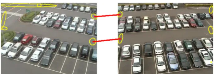
We also evaluate our method in an outdoor environment, a parking lot, with two cameras. Figure 10 shows the environment and the valid links determined by our method. The overall tracking accuracy is 89.4% by using unseen ground-truth of half an hour. It shows that our method performs well and achieves high tracking accuracy in both indoor and outdoor environments.
Figure 10. An outdoor environment, a parking lot, with two cameras, and the estimated entry/exit zones and valid links.
6. Conclusion
Unlike the other approaches assuming that the monitored environments remain unchanged, we have presented an adaptive and unsupervised method for learning both spatio-temporal and appearance relationships for a camera network. It can incrementally refine the clustering results of the entry/exit zones, and learns the appearance relationship in a short period of time by combing the spatio-temporal information and efficient MCMC sampling. We introduced a tracking algorithm, which takes advantage of the Gaussian mixture model learned for the entry/exit zones to enhance the tracking results. The experiments have shown that our method performs well, and high tracking accuracy can be achieved in both indoor and outdoor environments. Our method can re-build the appearance relationship models soon after sudden lighting changes, which is important for real situations and, to our knowledge, not achieved by the previous methods.
Acknowledgements
This work was supported in part by the Excellent Research Projects of National Taiwan University, under grant 95R0062-AE00-02, and by the National Science Council, Taiwan, under grants NSC 96-2752-E-002-007 -PAE.
References
[1] Q. Cai and J. K. Aggarwal. Tracking human motion in structured environments using a distributed-camera system. IEEE Trans. PAMI, 21(11):1241-1247, Nov. 1999.
[2] R. Collins, A. Lipton, H. Fujiyoshi, and T. Kanade. Algorithms for cooperative multisensor surveillance. Proceedings of the IEEE, 89(10):1456-1477, Oct. 2001. [3] D. Comaniciu, V. Ramesh, and P. Meer. Real-time tracking
of non-rigid objects using mean shift. In CVPR, 2000. [4] F. Dellaert. Addressing the correspondence problem: A
Markov Chain Monte Carlo approach. Technical report, Carnegie Mellon University School of Computer Science, 2000.
[5] A. Dempster, N. Laird, and D. Rubin. Maximum likelihood from incomplete data via the EM algorithm. Journal of the Royal Statistical Society, B-39(1):1-38, 1977.
[6] A. Dick and M. Brooks. A stochastic approach to tracking objects across multiple cameras. Proceedings of the Australian Conference on Artificial Intelligence, 2004. [7] A. Gilbert and R. Bowden. Tracking objects across cameras
by incrementally learning inter-camera color calibration and patterns of activity. In ECCV, 2006.
[8] W. K. Hastings. Monte Carlo sampling methods using Markov chains and their applications. Biometrika, 57, 1970. [9] T. Huang and S. Russell. Object identification in a Bayesian
Context. In IJCAI, 1997.
[10] O. Javed, Z. Rasheed, K. Shafique, and M. Shah. Tracking across multiple cameras with disjoint views. In ICCV, 2003. [11] O. Javed, K. Shafique, and M. Shah. Appearance modeling for tracking in multiple non-overlapping cameras. In CVPR, 2005.
[12] V. Kettnaker and R. Zabih. Bayesian multi-camera surveillance. In CVPR, 1999.
[13] S. Khan and M. Shah. Consistent labeling of tracked objects in multiple cameras with overlapping fields of view. IEEE Trans. PAMI, 25(10):1355-1360, Oct. 2003.
[14] D. Makris and T. Ellis. Automatic learning of an activity-based semantic scene model. In AVSS, 2003. [15] D. Makris, T. Ellis, and J. Black. Bridging the gaps between
cameras. In CVPR, 2004.
[16] A. Mittal and D. Huttenlocher. Scene modeling for wide area surveillance and image synthesis. In CVPR, 2000.
[17] H. T. Nguyen and A. W. M. Smeulders. Multiple target tracking by incremental probabilistic PCA. IEEE Trans. PAMI, 29(1):52 - 64, 2007.
[18] N. Otsu. A Threshold Selection Method from Gray-Level Histograms. IEEE Trans. on Systems, Man, and Cybernetics, Vol. SMC-9, NO.1, pp.62-66,1979.
[19] H. Pasula, S. Rusell, M. Ostland, and Y. Ritov. Tracking many objects with many sensors. In IJCAI, 1999.
[20] F. Porikli and A. Divakaran. Multi-camera calibration, object tracking and query generation. In ICME, 2003.
[21] M. Song and H. Wang. Highly efficient incremental estimation of Gaussian Mixture Models for online data stream clustering. Proceedings of SPIE Conference on Intelligent Computing: Theory and Applications III, 2005. [22] C. Stauffer. Learning to track objects through unobserved
regions. In WMVC, 2005.
[23] C. Stauffer and W. E. L. Grimson. Learning patterns of activity using real-time tracking. IEEE Trans. PAMI, 22(8):747-757, Aug. 2000.
[24] C. Stauffer and K. Tieu. Automated multi-camera planar tracking correspondence modeling. In CVPR, 2003.
[25] K. Tieu, G. Dalley, and W. Grimson. Inference of non-overlapping camera network topology by measuring statistical dependence. In ICCV, 2005.
[26] M. E. Tipping and C. M. Bishop. Probabilistic principal component analysis. Journal of the Royal Statistical Society, Series B, 61(3):611-622, 1999.