Analysis of Wave Propagation in Infinite Piezoelectric Plates

ANALYSIS OF WAVE PROPAGATION IN INFINITE PIEZOELECTRIC PLATES

C. Y. Wu * _{J. S. Chang} ** _{K. C. Wu} **

Institute of Applied Mechanics National Taiwan University Taipei, Taiwan 10617, R.O.C.

ABSTRACT

An analysis is presented for wave propagation in infinite homogeneous elastic plates of piezoelectric materials. The analysis is an extension to the work by Shuvalov [1] on wave propagation in general anisotropic elastic plates. A real form of dispersion equation is provided for a piezoelectric plate subjected to different boundary conditions on the plate surfaces. Perturbation theory [2] is exploited to obtain long-wavelength low-frequency approximation for physical quantities of wave propagation, including wave amplitude, stress, electric potential, electric displacement and velocity.

Keywords : Piezoelectric plates, Elastic waves, Stroh’s formalism, Perturbation method. 1. INTRODUCTION

Because of their unique ability to convert mechanical energy to electric energy and vise versa, piezoelectric materials are widely used as high-efficiency wave filter, voltage transformer, detecting device and actuator, etc. All these applications are connected with the vibration and wave propagation of piezoelectric materials. There are many papers related to wave propagation in piezoelectric plates under different boundary conditions. However, most works assumed either power series [3] or trigonometric series [4] for displacement field and electric field along the thickness direction. In this approach, multiple progression and superposition are needed in order to obtain the final results and the process becomes very tedious for materials of arbitrary anisotropy.

In this paper wave propagation in an infinite piezoelectric plate subjected to various boundary conditions is treated using an approach, which is an extension to the method developed by Shuvalov [1] for the same problem but without piezoelectricity. Shuvalov’s method is based on Stroh’s formalism for anisotropic elasticity. A distinctive feature of Stroh’s formalism is that the general solution is provided in terms of the eigenvalues and eigenvectors of an eigenvalue problem. Real-formed solutions can often be found by taking advantage of the orthogonality relations among the eigenvectors.

2. STROH’S FORMALSIM

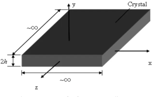
Consider a free disturbance harmonically propagating along x-direction parallel to the faces of an infinite

homogeneous piezoelectric plate with uniform thickness 2h (see Fig. 1). Elastic field and electro-magnetic field

are coupled in the piezoelectric plate. The corre- sponding vector fields of displacements u(x, y, t) and

potential ϕ (x, y, t) can be written as

( ) ( , , )_{x y t =} ( , )_{x y e}− ωi t ₌ ( )_{y e}i kx−ωt u u a (1) ( ) 4 ( , , )_{x y t} ( , )_{x y e}− ωi t _{a y e}( ) i kx−ωt ϕ ≡ ϕ = (2)

where k is the wave number, ω = kv is the frequency,

and v is the tracing velocity. The governing equation

under quasi-static approximation may be expressed as ,11+( + T) ,12+ ,22 = ρˆ QU R R U TU IU (3) where _{U u=[} T _{φ ≡]}T _{A( )y e}i kx( −ωt) _extended displacement, 1 0 0 0 0 1 0 0 ˆ 0 0 1 0 0 0 0 0 ⎡ ⎤ ⎢ ⎥ ⎢ ⎥ =_{⎢ ⎥} ⎢ ⎥ ⎣ ⎦ I .

Here the matrices Q, R, and T are given by

11 21 22 11 11 12 12 22 22 , , E E E T T T ⎡ ⎤ ⎡ ⎤ ⎡ ⎤ =_{⎢ ⎥} =_{⎢ ⎥} =_{⎢ ⎥} −ε −ε −ε ⎣ ⎦ ⎣ ⎦ ⎣ ⎦ Q e R e T e Q R T e e e (4) where QikE =Ci k1 1, RikE=Ci k1 2, TikE=Ci k2 2, i, k = 1, 2,

3, and Cijks are the elastic constants.; (eij)s = eijs, s = 1, 2, 3 and eijs are the piezoelectric stress constants; εij are the permittivity constants.

Fig. 1 Frame of reference coordinates Introduce the extended traction t2 as

( ) 2≡[ 2T D2]T = T ,1+ ,2 ≡ −ik y e( ) i kx−ωt

t σ R U TU B (5)

where σ2 is the stress vector on the plane normal to the

x2-axis, D2 is the x2-component of the electric displacement, and ( )_y T i d

k dy

≡ − + A

B R A T . In the

framework of the Stroh’s formalism, Eqs. (3) and (5) can be incorporated into a system of eight linear differential Eq. (5) as follows

( ) ( ) ( ) ( ) y y d _ik y y dy ⎡ ⎤₌ ⎡ ⎤ ⎢ ⎥ ⎢ ⎥ ⎣ ⎦ ⎣ ⎦ A A N B B (6)

Here the 8 × 8 real matrix N = N(v) is given by

1 2 2 3 ˆ 1 T T v ⎡ ⎤ ⎡ ⎤ ⎡ ⎤ =⎢ _{− ρ} ⎥ ⎢=_⎣ ⎥_⎦ ⎢_⎣ ⎥_⎦ ⎣ ⎦ N N 0 I 0 I N N I 0 I 0 N I N (7) where N1 = −T−1RT, N2 = −T−1, N3 = Q −RT−1RT, 0 and

I, respectively, are the 4 × 4 zero and identity matrices.

The matrices N1 and N3 have the following properties: [5]

1 2 = − 1, 3 2=0.

N e e N e (8)

where e1 = [1 0 0 0]T and e2 = [0 1 0 0]T. Let p and ξ be the Stroh eigenvalue and eigenvector,

respectively, of N, i.e., p =

Nξ ξ (9)

In consequence of the property (6) of N, linear

independent Stroh eigenvectors ξα, ξβ are orthogonal in the sense ξαTJξβ = 0, α≠β. If N is semi-simple, that is if it has a complete set of eight linear independent eigenvectors ξα (α= 1 ~ 8), then the solution of Eq. (6) is the superposition [5] 8 1 ( ) ( ) ikp y y C e y α= α α α ⎡ ⎤₌ ⎢ ⎥ ⎣ ⎦

∑

A ξ B (10)

where partial amplitudes Cα are determined (to within a common multiplier) by the boundary conditions. The

Stroh eigenvectors can be normalized such that 8

,

Τ Τ

αJ β= δαβ β αJ I=

ξ ξ ξ ξ (11)

where I8 is the 8 × 8 identity matrix.

3. DISPERSION RELATION

Equation (10) for y = −h becomes

8 1 ( ) ( ) ikp h h C e h α − α α α= − ⎡ ⎤₌ ⎢ ₋ ⎥ ⎣ ⎦

∑

A ξ B (12)

From Eqs. (11) and (12), Cα may be expressed as

( ) ( ) ikp h T h C e h α α= α ⎡⎢ − ⎤⎥ − ⎣ ⎦ A ξ J B (13)

Substitution of Eq. (13) into Eq. (10) leads to,

( ) ( ) ( , ) ( ) ( ) y h y h y h − ⎡ ⎤_{= −} ⎡ ⎤ ⎢ ⎥ ⎢ ₋ ⎥ ⎣ ⎦ ⎣ ⎦ A A M B B (14) where ( ) 8 1 2 3 1 1 ( , ) ( , ) ( , ) ( , ) ( , ) ikp y h T T y h y h y h e y h y h α + α α α= − − ⎡ ⎤ − = _{≡ ⎢ ⎥} − − ⎣ ⎦

∑

M M M J M M ξ ξ (15) Let the boundary conditions on the surface at y = − h

be given by

( )h ( )h

− − + − − =

X A Y B 0 (16)

where X− and Y− are constant matrices satisfying

, . T T T T − −+ − − = − − + − − = X X Y Y I X Y Y X 0 (17) It follows that ( )_h T , ( )_h T − − − = − = A Y g B X g (18)

where g is a nonzero constant column matrix.

Similarly let the boundary conditions on the surface at y

= h be given by

( )h ( )h

+ + + =

X A Y B 0 (19)

where X+ and Y+ are constant matrices. Substitution of Eq. (18) into Eq.(14), Eq. (19) yields

(X M+ 1( ,h h− )Y−T+X M+ 2( ,h h− )XT− 3( , ) 1( , ) ) T T T h h h h + − + − +Y M − Y +Y M − X g 0= (20)

Equation (20) gives the dispersion equation in the form det (X M+ 1( ,h h− )Y−T +X M+ 2( ,h h− )XT−

Consider the following three types of boundary conditions:

1. The mechanical boundary conditions are rigid and the electrical boundary conditions are short-circuit at the bottom and top surfaces. This is an extended definition of “fixed-fixed” boundary conditions for purely elastic plates. In this case X− = X+ = I, Y− = Y+= 0 and Eq. (21) reduces to

2

det (M ( ,h h− )) 0= (22)

2. The mechanical boundary conditions are stress-free and the electrical boundary conditions are open- circuit at the bottom and top surfaces. This is a definition corresponding to “free-free” boundary conditions for purely elastic plates. The boundary conditions are specified by letting X− = X+ = 0, Y− =

Y+= I and Eq. (21) becomes 3

det (M ( ,h h− )) 0= (23)

3. The mechanical boundary conditions are stress-free and the electrical boundary conditions are open- circuit at the bottom surface while the mechanical boundary conditions are rigid and the electrical boundary conditions are short-circuit at the top surface such that X− = Y+ = 0 and Y− = X+= I. This may be regarded as an extended definition of “free-fixed” boundary conditions for purely elastic plates. Equation (21) reduces to

1

det (M ( ,h h− )) 0.= (24)

4. CUT-OFF FREQUENCY

Consider normal incidence (k = 0, v→∞). Redefine

Eq. (1) as

( , )_{y t =} ( )_{y e}− ωi t

U A (25)

Substitution of Eq. (25) into Eq. (3) leads to 2 ,22= −ρω ˆ TA IA or 2 ,22 22 4,22 , E _{+ A = −ρω} T a e a (26) 22 ,22 22 4,22 0. T _{− ε A =} e a (27)

From Eq. (27), a4 can be expressed as

4 22 7 8 22 1 ( ) T ( ) , a y = y C y C+ + ε e a (28)

where C7 and C8 are constants. With Eq. (28), Eq. (26) becomes

2

,22 ,

E _{= −ρω}

T a a (29)

where TE =TE +e e22 22T /ε22 corresponds to the stiffened elastic constants. The solution of a(y) can be

expressed as 3 3 1 ( )_{y C e}ik yαy _{C e}−ik yαy , α α+ α α= ⎡ ⎤ =

∑

_⎣ + _⎦ a a (30)

where Cα are constants, kαy = ω/cα, α= 1 ~ 3, cα and aα, respectively, are the speeds and the corresponding polarization vectors of the stiffened acoustic plane waves propagating in the x2 − direction. Let

2= ,2= ( )y e− ωi t

t TU B (31)

Substitution of Eqs. (28) and (30) into Eq. (31) yields 3 3 22 7 1 ( )_{y C e}ik yαy _{C e}−ik yαy _{e C} α α+ α α= ⎡ ⎤ =

∑

_⎣ − _⎦ + b b (32) 4 22 7 B = −ε C (33) where bα = iρωcα aα.

The dispersion equations related to the three types of boundary conditions are discussed as follows:

1. “fixed-fixed” boundary conditions (A(−h) = 0 and A(h) = 0)

From Eqs. (28) and (30), the boundary conditions yield 3 3 7 8 0, 1, 2, 3, 0, 1, 2, 3, 0. y y y y ik h ik h ik h ik h C e C e C e C e C C α α α α − α α+ − α α+ ⎧ _{+ = α =} ⎪⎪ _{+ = α =} ⎨ ⎪ _{= =} ⎪⎩ (34) For nontrivial solutions of Cα, Eq. (34) gives

_ei k h2αy −_e−i k h2αy =₀ (35) The conditionforthecut-offfrequencies ( )n

α ω of standing- wave resonances is ( ) _{, 1, 2, 3, 0,1, 2,} 2 n n c _{n L} h α α π ω = α = = (36)

2. “free-free” boundary conditions (B(−h) = 0 and B(h) = 0)

From Eqs. (32) and (33), the boundary conditions yield 3 3 7 0, 1, 2, 3, 0, 1, 2, 3, 0. y y y y ik h ik h ik h ik h C e C e C e C e C α α α α − α α+ − α α+ ⎧ _{− = α =} ⎪⎪ _{− = α =} ⎨ ⎪ ₌ ⎪⎩ (37) From Eq.(37), the cut-off frequencies are the same as those given by Eq. (36) for type 1 boundary conditions. 3. “free-fixed” boundary conditions: (B(−h) = 0 and

A(h) = 0)

From Eqs. (28), (30), (32) and (33), the boundary conditions yield

3 3 7 8 0, 1,2,3, 0, 1,2,3, 0. y y y y ik h ik h ik h ik h C e C e C e C e C C α α α α − α α+ − α α+ ⎧ − = α = ⎪⎪ _{+ = α =} ⎨ ⎪ _{= =} ⎪⎩ (38) For nontrivial solutions of Cα, Eq. (38) gives

2 y 2 y ₀

i k h i k h

e α +e− α = (39)

The cut-off frequency related to free-fixed condition is

( ) (2 1) _{, 1, 2, 3, 0,1, 2,} 4 n n c _{n L} h α α + π ω = α = = (40)

Equations (36) and (40) are in the same form as those for purely elastic solids [1]. For piezoelectric solids, however, the wave speeds are calculated from the stiffened elastic constants.

5. LONG-WAVELENGTH APPROXIMATION

Consider the wave propagation in a “free” plate under the long-wavelength condition kh << 1. In the

following discussions h = 1 is assumed for simplicity.

When k<< 1, Eq. (15) may be approximated as

8 2 8 1 (1, 1) T _eikpα α α α= − =

∑

≈ M ξ ξ J I ₂ 1_{(2 )}2 2 1_{(2 )}3 3 2 6 ik ik ik + N+ N + N (41)

and the corresponding M3(1, −1) as 3(1, 1) 2− ≈ ik k( , )λ M D (42) where λ=ρv2, 2 3 2 ( , ) ( ) ( ) ( ) ( ) 3 k λ = λ +ik λ − k λ D N P Q (43) 3( )λ = 3− λˆ N N I (44) 3 1 1 3 ( )_{λ =} ( )_{λ +} T ( )_λ P N N N N (45) ( ) 2 3( ) 1 1T 3( ) 1 λ = λ + λ Q N N N N N 2 3( ) 2 3( ) ( 1T) 3( ) +N λ N N λ + N N λ (46)

From Eq.(42), Eq. (20) becomes

( , ) ( , )k λ k λ = D q 0 (47) where ( 1) ≡ − q A (48)

The limiting value of λ, denoted by λ0, as k → 0 is obtained by

0 0 0 3 0 0 0

(0, ) ( )λ λ = ( ) ( )λ λ =

D q N q 0 (49)

where q0( )λ ≡q(0, )λ . From Eq. (44), Eq. (49) can also be expressed as

3 0= λ0ˆ 0

N q Iq (50)

Equation (50) can be further written as 3 3 0 3 4 0 4 0 0 1 ( ) ( )ij j ( ) ( )i ( ) ,i 1, 2, 3, j i = + = λ =

∑

N q N q q (51) and 3 4 0 3 44 0 4 ( ) ( )N j q j+( ) ( )N q =0 (52)

where (N3)ij and (q0)j denote, respectively, the elements of N3 and q0. From Eq. (52), (q0)4 may be expressed as 3 4 0 4 0 3 44 ( ) ( ) ( ) ( ) j j = − N q q N (53)

Substitution of Eq. (53) into Eq. (51) leads to 3 3 0 0 0 1 ( ) ( )ij j ( ) ,i 1, 2, 3 j i = = λ =

∑

N q q (54) where 3 4 3 4 3 3 3 44 ( ) ( ) ( ) ( ) ( ) i j ij = ij− N N N N N (55)

It follows from Eq. (8) that (N3)i2 = (N3)2i = 0, i = 1 ~ 4 and hence ( )N3 2i =( )N3 2i =0. The eigenvalues of Eq. (54) are (2) (1) (3) 0 0, 0 , 0 1₂⎡ ( )3 11 ( )3 33 λ = λ λ = _{⎣ N} + N

(

)

2 ₂ 3 11 3 33 3 13 ( ) ( ) 4( ) ⎤ ± N − N + N _⎥⎦ (56)

The eigenvalues correspond to the limiting values of the speeds of the three fundamental waves in a free plate. The matrix ( )

0i

q , i = 1,2,3, can be obtained from the

eigenvector of Eq. (54) corresponding to ( ) 0i λ and Eq. (53). In particular, (2) 0 = 2. q e Define (4) 0 = 4= q e

[0 0 0 1]T. It may be shown that ( ) ( ) 0αT ˆ0β = δαβ, α =1 4, β =1 4 q q ∼ ∼ (57) where ( ) ( ) 0 ˆ 0 ˆ α ₌ α, q Iq α= 1, 2, 3,and (4) (4) 0 3 0 3 44 ˆ = /( ) q N q N .

4 ( ) ( ) 0 0 1 ˆ ( )T α α α= =

∑

q q I (58)

and N3(λ) admits the following representation 3 ( ) ( ) ( ) (4) (4) 3 0 0 0 3 44 0 0 1 ˆ ˆ ˆ ˆ ( ) ( α ) α( α )T ( ) ( )T α= λ =

∑

λ − λ + N q q N q q (59)

For future use, a pseudo-inverse of N3 (λ0(β)) is given by 3 ( ) 1 ( ) ( ) (4) (4) 3 0 ( ) ( ) 0 0 3 44 0 0 1 0 0 1 ( α <− >) β ( β)T ( ) ( )T β α β= β≠α λ = + λ − λ

∑

N q q N q q (60) The limiting value of the first derivative of λ with

respect to k, denoted by λ0′, as k → 0 can be derived by considering 0 { ( , ) ( , )} { ( , ) ( , )} d _{k k k k} dk k ∂ ∂ ⎛ _′ ⎞ λ λ =_⎜ + λ _⎟ λ λ = ∂ ∂λ ⎝ ⎠ D q D q 0 (61) at k = 0 and λ= λ0. Substitution of Eq. (43) into Eq.

(61) gives 0 0 0 3 0 0 3 0 0 0 ˆ ( ) ( ) ( ) k i k = λ=λ ⎛ ⎞ ∂ ∂ _′ λ + λ _∂ + − +⎜_⎜ λ _∂λ ⎟_⎟λ = ⎝ ⎠ q q P q N q N 0 (62) Pre-multiplying Eq. (62) by qT0 and using Eq. (49), we

get

( ) ( ) ( ) ( ) 0α′ i 0αT ( 0α) 0α 0

λ = q P λ q = (63)

With Eq. (63), Eq. (62) leads to 1 ( ) ( ) ( ) 3 0 0 0 0 ( ) ( ) ( ) 1 0 1 0 0 ( ) ( ) ˆ { [( ) ]} , k T i k i α <− > α α α = α α α ∂ _{= − λ λ} ∂ = − − q _{N P q} N I q N q q (64) where Eqs. (59) and (60) has been used.

Similarly, the limiting value of the second derivative of λ with respect to k, denoted by λ0″, as k→ 0 can be obtained by considering T 22{ ( , ) ( , )} d _{k k} dk λ λ q D q T 2{ ( , ) ( , )} 0_{k k} k ∂ ∂ ⎛ _′ ⎞ = _⎜ + λ _⎟ λ λ = ∂ ∂λ ⎝ ⎠ q D q (65)

at k = 0 and λ=λ0. With Eqs. (49) and (63), Eq. (65) yields ( ) ( ) ( ) ( ) ( ) ( ) ( ) 0 0 0 0 0 0 0 4 _{( ) 2 ( )} 3 T T k i k α α α α α α α = ∂ ′′ λ = − λ + λ ∂ q q Q q q P (66)

Equation (66) can be simplified by substituting Eq. (64) into Eq. (66) and using Eq. (49). The result is

( ) 3 ( ) ( ) ( ) ( ) 2 0 0 0 0 1 0 1 2 _{( )(ˆ )} 3 T α β α β α β= ⎧⎪ ′′ λ = ⎨ λ − λ ⎪⎩

∑

q N q (4) ( ) 2 3 44 ˆ0 1 0 ( ) ( T α) ⎫ + _⎬ ⎭ N q N q (67)

In particular, Eq. (67) for α = 2 can be reduced to a

remarkably simple form ( )

0α′′ 2 ( )₃ 3 11

λ = N (68)

where Eq. (8) has been used.

From Eqs. (56), (63), and (67), the velocities vα, α= 1, 3, are given by 2 ( ) ( ) ( ) 0 0 ( ) 0 1 4 k vα vα α α ⎛ λ ′′⎞ ⎜ ⎟ = _⎜ + _⎟ λ ⎝ ⎠ (69) where ( ) ( ) 0 0 vα ₌ λα ρ (70)

From Eqs. (56), (63), and (68) the expression for v(2) is given by (2) ( )3 11 3 v =k ρ N ₍₇₁₎

Equation (71) is in the same form as that for purely elastic solids.

The extended displacement and traction amplitudes

A(y), B(y) at k<< 1 can be expressed as 3 3 ( ) ( ) 1 1 ( )y D α ( ),y ( )y D α( )y α α α= α= =

∑

=

∑

A A B B (72)

where Dα are disposable normalization factors, A(α)(y) and B(α)_{(y), respectively, are the extended displacement} and traction amplitudes corresponding to the three fundamental waves. By Eqs. (14), (41), and (42), to the first order in k,

( ) ( ) ( ) 1 0 0 ( ) ( ) ( ) 3 0 0 ( ) [ ( 1) ] , ( ) ( 1) ( ) ( 1) ( ) . 2 k k y ik y k k ik y ik y v y v k k α α α α = α α α α = ⎧ _{= + +} ⎛ ₊ ∂ ⎞ ⎪ ⎜_{⎜ ∂} ⎟_⎟ ⎪⎪ ⎝ ⎠ ⎨ ⎛ ⎞ ⎪ _{= +} ⎡ _{+ +} ⎤_{⎜ +} ∂ _⎟ ⎪ ⎢_⎣ ⎥⎜_{⎦ ∂} ⎟ ⎪ ⎝ ⎠ ⎩ q A I N q q B N P q (73) Substitution of Eq. (64) into Eq. (73) gives

(2) 2 1 ( )y = −iky A e e (74)

(

)

(1,3) (1,3) (1,3) (1,3) (1,3) 0 1 ˆ0 1 0 4 0 ( )_{y = +ik y⎡ +} T _⎤ ⎣ ⎦ A q N q N q I q (75)

(2) 2 2 3 1 ( ) ( 1) 2 k y = y − B N e (76) (1,3) 2 2 (1,3) (1,3) 3 1 0 ( ) (1 ) ( ) 2 k y = −y v B N N q (77)

Equations (74) ~ (77) reveal the general property that, for any of the three fundamental wave branches, the extended traction taken in the leading approximation is orthogonal to the limiting polarization of the corresponding extended displacement,

( ) ( ) 0 ( )y 0, 1, 3, 1 y 1 α _⋅ α _{= α = − ≤ ≤} B A 　 　 (78) 6. CONCLUSION

A theoretical framework developed by Shuvalov [1] for wave propagation in infinite homogeneous anisotropic elastic plates has been extended to piezoelectric plates. Dispersion equations have been derived for general boundary conditions on the plate surfaces. Special cases corresponding to fixed-fixed, free-free, and free-fixed conditions for elastic plates were discussed and cut-off frequencies derived. Perturbation theory was exploited to obtain long- wavelength physical quantities of wave propagation

including wave amplitude, stress, electric potential, electric displacement and velocity for a “free” piezoelectric plate.

REFERENCES

1. Shuvalov, A. L., “On the Theory of Wave Propagation in Anisotropic Plates,” Proc. Soc. Lond. A., 456, pp. 2197−2222 (2000).

2. Stewart, G. W. and Ji-guang Sun, Matrix

Perturbation Theory, Academic Press, Inc. (1990).

3. Kaul, R. K. and Mindlin, R. D., “Frequency Spectrum of a Monoclinic Crystal Plate,” J.

Acoust. Soc. Am., 34, pp. 1902−1910 (1961).

4. Lee, P. C., Syngellakis, Y. S. and Hou, J. P., “A Two-Dimensional Theory for High-Frequency Vibration of Piezoelectric Crystal Plates with or without Electrodes,” Journal of applied Physics

61, pp. 134−141 (1987).

5. Ting, T. C. T., Anisotropic Elasticity, Oxford University Press (1996).

(Manuscript received March 4, 2005, accepted for publication May 18, 2005.)