Experiments on Deposition Behavior of Fine Sediment in a Reservoir

E

XPERIMENTS ON

D

EPOSITION

B

EHAVIOR OF

F

INE

S

EDIMENT

IN A

R

ESERVOIR

By Wei-Sheng Yu,

Hong-Yuan Lee,

and ShaoHua Marko Hsu

ABSTRACT: The deposition behavior of fine sediment is an important phenomenon, and yet it is unclear to engineers concerned about reservoir sedimentation. Laboratory experiments were conducted to produce both quasi-homogeneous flow and a turbidity current region divided by a plunge section. Silica powder (a noncohesive sediment) and kaolin (a cohesive sediment) were used as the suspended material. Because the effective gravi-tational force is the primary driving force for velocity in turbidity currents, the velocity profile was closely related to the concentration profile. The deposition rate of noncohesive coarser particles exponentially decays along the flow path. Most of the coarser particles were deposited in the quasi-homogeneous flow region or within a small distance downstream of the plunge section. The plunge did not carry those coarser particles further downstream. Deposition in the region of the turbidity current was found mainly by cohesive particles. Hydraulic sorting exists in the quasi-homogeneous flow region for noncohesive coarser particles, but becomes less significant in the downstream portion with deposition rates becoming mildly decayed. For fine cohesive particles, hydraulic sorting for the deposited gradation is not significant.

INTRODUCTION

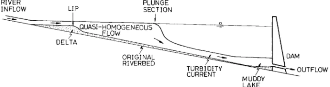
Depending upon the sediment supply from the watershed and flow intensity in terms of velocity and turbulence, river flows usually carry sediment particles within a wide range of sizes. When a river flows into a reservoir, the coarser particles deposit gradually and form a delta in the headwater area of the reservoir that extends further into the reservoir as deposi-tion continues (Fig. 1). Finer particles, being suspended, flow through the delta stream (Fig. 1) and pass the lip point of the delta, first entering a quasi-homogeneous (nonstratified) flow region and subsequently being deposited along the path due to a decrease in flow velocity caused by the increased cross-sectional area. The region of quasi-homogeneous flow is shorter in cases of smaller discharge and/or higher sediment concentration. On the contrary, the region of quasi-homoge-neous flow is longer in cases of larger discharge and/or lower sediment concentration. Until the section-averaged densimetric Froude number become about 0.6 – 1.0 (Lee and Yu 1997), the sediment-laden flow will plunge into the water body and move along the bed surface to form a turbidity current (or gravity current). The location of the plunge section can be easily iden-tified in experiments by a distinct clear upper layer of ambient water against a turbid layer beneath the ambient water. A re-verse flow, carrying suspended debris in the ambient upper layer, can also be observed. As it moves downward, the tur-bidity current can either deposit onto or erode the bed surface depending upon various factors.

For certain situations, the turbidity current, carrying silt and clay, can move for several tens of kilometers (Fan and Morris 1992). If the turbid inflow continuously flows into a reservoir, the turbidity current will sustain itself and arrive at the dam site. When it hits the dam, the turbidity current can soar up, and a muddy lake then forms. Fig. 1 is a schematic represen-tation for a deposition delta, quasi-homogeneous flow region, turbidity current region, and a muddy lake. The deposition behavior in quasi-homogeneous flow region is not usually

1

Assoc. Res. Sci., Environment Div., Agric. Engrg. Res. Ctr., Chungli 320, Taiwan.

2

Prof., Dept. of Civ. Engrg., Nat. Taiwan Univ., Taipei, Taiwan.

3_{Assoc. Prof., Dept. of Hydr. Engrg., Feng Chia Univ., Taichung 407,}

Taiwan.

Note. Discussion open until May 1, 2001. To extend the closing date one month, a written request must be filed with the ASCE Manager of Journals. The manuscript for this paper was submitted for review and possible publication on February 25, 1999. This paper is part of the

Jour-nal of Hydraulic Engineering, Vol. 126, No. 12, December, 2000.

䉷ASCE, ISSN 0733-9429/00/0012-0912–0920/$8.00 ⫹ $.50 per page.

Paper No. 20418.

mentioned in the existing literature. The writers believe that a description of the entire deposition system is not complete without this portion. According to the above description, the deposition behavior of reservoir sediment relates closely to the size of the particles and flow patterns in the reservoir. Four categories of deposition can be distinguished: (1) Coarse-par-ticle deposition in the delta; (2) fine-parCoarse-par-ticle deposition in the quasi-homogeneous flow region; (3) finest-particle deposition in the turbidity current region; and (4) finest-particle deposi-tion in the muddy lake region. Categories 2 and 3 are the focus of this paper.

In a pioneer experiment on turbidity current with a hori-zontal bed using plastic beads with a density of 1.52 g/cm3

and a median particle size of 0.18 mm, Middleton (1967) found that sorting exists in the longitudinal, vertical, and lat-eral directions. By creating turbidity currents inside a flume with a slope of 0.05, Garcia (1985) observed that in most cases of his experiments, the coarsest portion of the sediment could not be kept in suspension and tended to settle down near the inlet region. In a series of experiments with a slope between 0 and 0.056, using quartz flour with a median diameter of 0.014 and 0.032 mm, Altinakar et al. (1990) found that the deposition effect slows down the marching velocity and in-creases the thickness of the head portion of the turbidity cur-rent. Garcia (1993) studied the transition process (hydraulic jump) between supercritical and subcritical turbidity currents, in which the bed slope was 0.08 for the supercritical portion and horizontal for the subcritical portion. In a case presented by Garcia (1993) involving a silica-laden flow (with a density of 2.65 g/cm3

and a geometric mean of particles 0.004 and 0.009 mm, respectively), the amount of deposition in the two portions did not show any significant difference. While in a case involving glass beads (with a density of 2.50 g/cm3 _and

a geometric mean of particles 0.030 and 0.065 mm, respec-tively) of a larger size, deposition begins at the inlet of the supercritical region and decays exponentially with the distance traveled.

The flow fields of turbidity current in the aforementioned literature were all controlled using sluice gates, and no plunge phenomenon occurred. In nature, however, plunge is an essen-tial part in the whole system and cannot be overlooked. The effect of plunge upon the behavior of deposition in a reservoir is not clearly understood at present. Until now, only a few discussions have been conducted on the deposition of fine par-ticles in a quasi-homogeneous flow region and the turbidity current region. The difference due to the cohesive effects be-tween fine particles has not been discussed yet.

quasi-FIG. 1. Schematic Diagram for Flow Types of Sediment-Laden Water in Reservoir

FIG. 2. Grain-Size Distribution Curves for Kaolin and Silt, Re-spectively

homogeneous flow and the stratified turbidity current. Two types of sedimentary material were used: silica, a noncohesive material, and kaolin, a cohesive material. The topics focused upon are (1) comparison of the velocity and concentration pro-files among the quasi-homogeneous flow, depositing turbidity current and nondepositing turbidity current; (2) the deposition process and gradation of cohesive or noncohesive deposited materials in the quasi-homogeneous flow region; (3) the dep-osition process and particle gradation of both cohesive and noncohesive material in the stratified turbidity-current region; and (4) comparison of the deposition amounts and gradation of the deposited materials between the upstream and down-stream plunge sections.

EXPERIMENTAL APPARATUS AND PROCEDURE

Experiments were conducted in a transparent flume, 20-m long, 20-cm wide, and 60-cm high, with a bottom slope of 0.02. A cylindrical mixing tank with volume of 1.2 m3

was used for mixing sediment and water, which can supply all of the turbid-water inflow during one run.

Two head tanks, for clear water and turbid water, respec-tively, were installed. The turbid-water head tank has two con-centric cylinders. The turbid water was pumped from the mix-ing tank to the inner tank of the turbid-water head tank. When the inner tank was full, the turbid water overflowed from the inner tank into the outer tank of the turbid-water head tank, and then the turbid water within the outer tank was quickly drained, by bottom valves, into the mixing tank. Mixers with a variable-speed motor were used in the inner tank of the tur-bid-water head tank and the mixing tank to keep the sediment in suspension. Turbid water was supplied into the flume, after the inner tank overflowed, by several near-bottom valves under the inner tank of the turbid-water head tank. A receiving tank was installed on the downstream end to detain the turbid water and drain it through an overflow weir and a bottom valve. The 20-m-long flume was divided into two parts. A 4-m-long sec-tion for the open channel region, and a 16-m-long secsec-tion for the backwater region. The layout of the flume can be found in a work by Lee and Yu (1997).

A magnetic current meter, with an accuracy of⫾0.5 cm/s, was used to measure flow velocity. The diameter of the current meter is 0.9 cm, and the length is 2.8 cm. The magnetic field is interfered by the channel bottom and walls, and hence the current meters cannot be used in the near-wall region (2 cm from the channel walls and 1 cm from the channel bottom). Siphon-type suction tubes with a diameter of 3.5 mm were used to take concentration samples. During the sampling pro-cess, the withdrawal velocity was set to be approximately equal to the flow velocity. An electronic balance with an ac-curacy of 0.0001 g was used to weigh the samples.

The suspended materials used were silica and kaolin with a specific gravity of 2.66 and 2.65, respectively. The median particle diameter was 0.05 and 0.0068 mm, respectively. The average particle fall velocities were 0.3950 and 0.0106 cm/s, respectively. Grain sizes larger than 0.074 mm (dimension of #200 U.S. standard sieve) were measured using sieve analysis.

Grain sizes smaller than 0.074 mm were measured with a hy-drometer. The particle-size distribution curves for the silica and kaolin are shown in Fig. 2.

Dispersion agent was added in part of the experimental runs to inhibit the cohesive effects between fine particles, according to the ASTM D 422 hydrometer analysis method for analyzing size distribution for particles below sieve #200. For each 50 g of dry sample, a container with 200 cm3

of clear water should be used, and 1.5 g (or 3%) of dispersion agent should be added, mixed uniformly, and soaked for 18 h before the experiment. In other words, the mass ratio for dry sample, water, and dispersion agent is 100:325:3. For each run, a suf-ficient amount of turbid water should be prepared in the mix-ing tank for the whole run such that the concentration of the turbid water can be constant.

To begin the experiment, the flume was first filled with clear water to form a reservoir, and then turbid water was released from the head tank. The outflow discharge was set equal to the inflow discharge. The inflow discharge and its sediment concentration were kept constant during each experimental process.

Three groups of experiments were conducted. The experi-mental conditions for these groups are listed in Table 1, in which qi is the inflow discharge per unit width; C ,¯i

dimen-sionless by volume, is the inflow concentration of the sus-pended material; and T is the water temperature. All runs were depositing processes without erosion. Case A was designed to investigate the deposition behavior of silica in a quasi-homo-geneous flow region. Case B investigated the deposition be-havior of kaolin in a quasi-homogeneous flow region and a turbidity current region. Case C was conducted to investigate the difference in deposition between the upstream and down-stream plunge sections. A dispersing agent, sodium hexame-taphosphate, was added in all Case A runs as noncohesive behavior was being studied. For the same reason, a dispersing agent was also added in the three runs of Case C. In Cases B and C, quasi-homogeneous flow and turbidity current coex-isted in each experiment. In Case A, the discharge and con-centration were controlled to inhibit the occurrence of plunge. In all runs, the inflow discharge and inflow sediment concen-tration were recorded. The velocity of the marching head of the turbidity current was measured for calculating the

depo-TABLE 1. Experimental Conditions for All Cases Case (1) Flow type (2) Suspended materials (3) Run number (4) With dispersing agent (5) qi (cm2 /s) (6) ¯ Ci (dimensionless by volume) (7) Total sediment added in mixing tank (8) T (9)

A Quasi-homogeneous flow Silica HS1 HS2 HS3 HS4 ⻫ ⻫ ⻫ ⻫ 138.410 138.740 167.131 259.771 0.00185 0.00083 0.00170 0.00373 — — — — 23.2 23.4 23.4 22.0 B Both quasi-homogeneous

flow and turbidity cur-rent Kaolin HK1 HK2 X X 101.358 208.454 0.00144 0.00324 — — 18.0 19.8 C Both quasi-homogeneous

flow and turbidity cur-rent

Both silica and kaolin TP1 TP2 TP3 TP4 ⻫ ⻫ X ⻫ 68.989 68.263 68.653 68.842 0.00512 0.00748 0.00748 0.01596 20-kg silica 20-kg silica 10-kg kaolin 20-kg silica 10-kg kaolin 20-kg silica 50-kg kaolin 20.4 21.0 20.8 21.3

FIG. 3. Typical Concentration Profiles for Quasi-Homogene-ous Flow

FIG. 4. Typical Velocity and Concentration Profiles of Depos-ited Turbidity Current

sition time interval only on each sampling reach along the flow path. The velocity and concentration profiles were measured in some of the other runs, and the experimental conditions for those runs are not shown in Table 1. After each run was com-pleted, the water in the flume was drained slowly, and the amount and gradation of the deposition along the distance was measured.

RESULTS AND ANALYSIS

Velocity and Concentration Profiles

Quasi-Homogeneous Flow

The velocity and concentration profiles for the quasi-homogeneous flow are similar to the open-channel flow pro-files, in which the larger the Rouse number, Ws/␬U_* (where

Ws is fall velocity of the suspended sediment; ␬ is the von

Ka´rma´n constant, and U

* is shear velocity), the more non-uniform the concentration profile and the suspended sediments tend to concentrate toward the channel bed. For the experi-ments in Case A, the quasi-homogeneous flow with silica sus-pension deposition occurred along the entire flume. In the up-stream portion, the rate of deposition was significant, and therefore the concentration near the bed was large. Toward the downstream portion, the size of the suspended particles be-came finer due to the lack of coarse particles. The rate of deposition slowed down, and the concentration profile became more uniform, vertically. The typical concentration profiles for the quasi-homogeneous flow are shown in Fig. 3, in which X is the distance form the flume entrance; and H is the water depth.

Turbidity Current

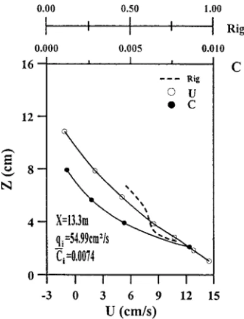
In the stratified flow, the kaolin turbidity current without a dispersing agent was deposited along the flow path due to its flocculation behavior. The velocity and concentration profiles in this deposition case are shown in Fig. 4, in which U, C, andRigare the velocity, concentration, and gradient

Richard-son number [definition referred to in (1)] at a local position, respectively; and Z is the vertical distance, normal to the bed, from the channel bed. On the contrary, kaolin with a dispersing agent (sodium hexametaphosphate) was not deposited. The ve-locity and concentration profiles for this nondeposition case are shown in Fig. 5. The difference between the profiles in Figs. 4 and 5 are obvious. The concentration profile gradient at the lower portion of the deposition case (Fig. 4) shows a highly nonuniform concentration with an increase near the bed. The corresponding velocity profile is also different from that of a normal open-channel flow. The high concentration

near the bed in Fig. 4 indicates an increase in the effective gravitational force quantified as g(s ⫺ 1)C sin ␪⌬Z, where g is the gravitational acceleration; s is the specific gravity of suspended solid;␪ is the angle of the bed slope; and ⌬Z is an element in the vertical direction, the gravitation term of the momentum equation for the turbidity current (Yu and Lee

FIG. 5. Typical Velocity and Concentration Profiles of Turbid-ity Current with Dispersing Agent

1993), increasing the velocity near the bed. This is a clear distinction between a stratified flow and an open-channel flow. In an open-channel flow, the velocity profile is not dominated by the concentration distribution. In addition, the lower portion of the concentration profile in the nondeposition case (Fig. 5) is nearly constant and is similar to that in an open-channel flow with a wash load. The velocity profile of the lower layer in Fig. 5 is also similar to that in an open-channel flow.

In a stratified flow, the gradient Richardson number is usu-ally a good indicator of the degree of unstableness at a local point. The definition of the gradient Richardson number is as follows: d␳m g dz Rig=⫺ 2cos␪ (1) dU ␳m

冉 冊

in which␳m = density of a point with a specified Z value;␳m

is equal to␳sC⫹ ␳a(1⫺ C) (where ␳sand␳aare the densities

of the suspended sediment and ambient fluid), respectively;

Rig is always positive. It is found that the larger the velocity

gradient dU/dZ, the smaller theRigbecomes, which indicates

greater instability and more local mixing. In Garcia’s super-critical flow experiments (Garcia 1993), the averaged value for

Rig is 0.16 at the interface between the ambient fluid and the

turbidity current, whereas, in the subcritical case, the similar value is 0.64. Garcia inferred that forRigvalues approximately

larger than 0.25, turbulence cannot be maintained against sta-ble stratification. He illustrated that his subcritical flows are stable, and mixing at the interface is negligible.

In Fig. 4 (the deposition case of turbidity current), theRig

values are between 0.46 and 0.78, which are all larger than 0.25. From Garcia’s inference as mentioned before, this indi-cates a stable condition in the deposition case, in which mixing between the clear and turbid water at the interface can be dis-regarded. In Fig. 5 (the case without deposition), the velocity and concentration decrease rapidly at the position above Z = 9 cm, at which the interface divides the turbidity current layer, and are obviously different as compared with the deposition case in Fig. 4.

Based on (1), which is the definition ofRig, point values of

Rig rely on the accuracy of the gradients for dC/dZ and

dU/dZ at each point. It is found that it is better to rely on the

fitted curve of C(Z) and U(Z) rather than measured point val-ues of C and U to obtain the gradients.

Eighteen runs of kaolin turbidity current with dispersing agent in a study by Lee and Yu (1997) showed that the simi-larity collapse is good for the velocity and concentration pro-files, and those can be fitted to (2) and (3), respectively

U _0.05 1 = 1.15(3␩) , 0 ⱕ ␩ ⱕ (2a) ¯ U 3 4 U 1 1 = 1.15 exp

冋 冉 冊册

where␩ = Z/h, in which h is the calculated thickness of tur-bidity current. The turtur-bidity current thickness, layer-averaged velocity, and layer-averaged concentration can be calculated from the measured velocity profile as follows (Ellison and Turner 1959, Parker et al. 1987):

␦ U dz

冕

冕

冕

冕

冕

in which␦ = distance between the channel bed and the posi-tion where the velocity equals zero; U¯ = layer-averaged tur-bidity current velocity; andC¯ = layer-averaged turbidity cur-rent concentration.

The bulk Richardson numberRi(Ellison and Turner 1959) can be defined as follows:

¯

g(s⫺ 1)cos ␪Ch

Ri= _¯2 (5)

U

Based on (1) and (5), the relationship betweenRig andRi

is as follows:

Rig= F (␩) ⫻Ri (6)

where F (␩) = function for the shape of gradient Richardson number ¯ d(C/C) d (Z/h) F (␩) = ⫺ 2 (7) ¯ d (U/U)

冋 册

Turner (1973) discussed the relationship between Rig and

Ri for several special circumstances. In this study, F(␩) can be specified based on the measured data. Selecting the zone across the interface (␩ ⬇ 1) and substituting (2b) and (3b) into (7), one can obtain

FIG. 6. Dimensionless Velocity, Concentration, and F(␩) Pro-files of Turbidity Current with Dispersing Agent

FIG. 8. Comparison of Deposition Patterns between Silica (Noncohesive) and Kaolin (Cohesive) Suspension in Quasi-Homogeneous Flow Region

FIG. 7. Deposition Rate and Median Diameter with Distance of Deposited Sediment (Run HS4)

1 (␩ ⫺ 0.6) _␣ F(␩) = 6e (8) 35.3511 (␩ ⫺ 0.3333) where ␣ = ⫺15.43(␩ ⫺ 0.6)2 ⫹ 15.4 (␩ ⫺ 0.3333)4 . Eqs. (2a), (2b), (3a), (3b), and (8) are plotted in Fig. 6. The deriv-ative of (8) is taken as follows:

dF(␩) 1 1

= ₇

d␩ 35.3511 (␩ ⫺ 0.3333)

5 4 3 2 ␣

⭈(61.6␩ ⫺ 119.1␩ ⫹ 59.5␩ ⫹ 13.6␩ ⫺ 22.2␩ ⫹ 6.5)e (9)

The minimum value of Rig can be found as ␩ = 1.01 by

solving (9) with␩ ranging between 0.6 and 1.2. This shows that the thickness of the turbidity current calculated by the velocity profile [(4)] is exactly at the position of the minimum

Rigvalue, in which the instability is maximum and the mixing

is nonnegligible. Hence,␩ = 1 can be used as a criterion to define the interface.

For the case of Fig. 5, the calculated thickness h is 12.8 cm; layer-averaged velocityU¯ is 8.93 cm/s; and layer-averaged concentrationC¯ in a dimensionless form by volume is 0.00291 (Lee and Yu 1997). Taking g = 980 cm2

/s, s = 12.65, and cos

␪ ⬇ 1, then substituting the above values of h, , andU¯ C¯ into (5), the calculated Ri value for the case of Fig. 5 is 0.76. Substituting theRivalue and the F(␩) of (8) into (6), one can obtain the profile of Rig at the region across the interface

(␩ ⬇ 1) for the case of Fig. 5. The calculatedRig is plotted

on Fig. 5, and theRig value is 0.17 at the interface. Because

the Rig value is smaller than 0.25, the mixing effect is not

negligible at the interface in the nondeposition case of turbid-ity current.

Deposition Rate

Definition of Deposition Rate

The deposition rate, WD, is the rate of the bed-elevation

increase within each flume reach without considering the po-rosity effect and can be calculated using the measured data as follows:

⌬W

W =D _{␥ B⌬x⌬t} (10)

s

where␥ = specific weight of the sediment; B = width of the flume; and⌬W = weight of the deposited sediment within the sampled segment ⌬X in the time interval ⌬t. The quantities on the right-hand side of (10) are all measurable. The

depo-sition rate for each size fraction can be obtained by multiply-ing (10) by the measured gradation of the deposited sediment.

Quasi-Homogeneous Flow

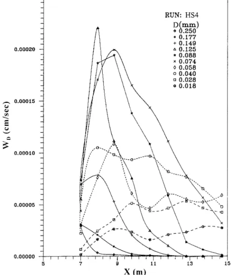
The quasi-homogeneous flow is between the downstream end of the deposition delta and the plunge section. Because the formation of a delta may take a long time, all of the ex-periments in Case A were terminated before a delta could be formed. A typical profile of the deposition rate for silica (Run HS4) is shown in Fig. 7, in which a peak value exists at X = 8.5 m and exponentially decays after the peak. The D50in Fig.

7 refers to the median diameters of deposited particles. In Fig. 7. the location of the peak deposition rate is 2 m downstream of the starting point of the backwater region. After the starting point, the deposition rate increased downward until the dep-osition-rate peak occurred. If sufficient time is permitted, a delta will gradually form between the starting point and the point of peak deposition rate (Yu et al. 2000). As a conse-quence, the effective sampling location for the quasi-homo-geneous flow is downstream of the peak. In Fig. 7, the dep-osition rate of quasi-homogeneous flow decays from 0.00107 to 0.00016 cm/s within a length of 8.9 m.

FIG. 10. Deposition Rate along Flow Distance in Case B FIG. 9. Deposition Rate along Flow Distance in Case C and noncohesive suspended sediments. The deposition rate for

noncohesive material decays exponentially along the path as previously stated. On the contrary, the deposition rate for co-hesive material increases along the path. The behavior of non-cohesive material is similar to cases of particle transportation without resuspension, which usually occurs in a settling basin (Camp 1946). Sumer (1977) also stated that the distribution of deposited particles follows an exponential decay function along the flowing path of a settling basin. The deposition of cohesive materials is due to the flocculation behavior between the sediment particles. As flow intensity decreases toward the downstream direction, the cohesive effect becomes relatively strong.

Plunge Effect on Deposition of Noncohesive Sediment In the homogeneous flow region, the deposition rate for noncohesive sediment follows an exponential decay as previ-ously stated. Under certain conditions, a plume occurs, and then a turbidity current forms. Runs TP1, TP2, and TP4 of Case C are cases for noncohesive suspended sediment. In these three runs, 20 kg of silica was used, but different amounts of kaolin were added. All of the sediment was added into the mixing tank and mixed with clear water using a variable speed motor. The sediment was kept suspended in the mixing tank, so that the inflow sediment concentration could be kept con-stant during each run. Run TP1 used no kaolin; Run TP2 used 10 kg of kaolin; and Run TP4 used 50 kg. In all three runs, a dispersing agent was used to eliminate the cohesive effects. From Lee and Yu (1997), the plunge criteria can be expressed as follows: 1/3 2 qp H =p ␤⭈

冉 冊

where Hp = water depth; ␤ = coefficient; qp = discharge per

unit width; g⬘p = effective gravitational acceleration; g⬘p = g(s ⫺ 1) ; andC¯p C¯p = cross-sectional-averaged concentration of the suspended sediment. The subscript p is just an index of the plunge section. Based on field and flume data, most re-searcher found that the〉 value was between 1.0 and 1.4 (Lee and Yu 1997), except for Wunderlich and Elder (1973), whose

␤ is 1.6. Based on flume experiments, Lee and Yu (1997)

stated that the downstream stage would affect the␤ value and make it larger than 1.4. Other factors are unsteady flow and reservoir geometry, as well as other minor factors. Based on the above statement, (11) could be used to approximately es-timate the plunging depth, even in the field.

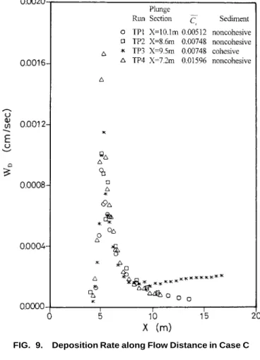
From (11), the location of the plunge section is obviously affected by the concentration. The higher the concentration, the earlier the plunge occurs. For Runs TP1, TP2, and TP4, the plunge section occurs at X = 10.1, 8.6, and 7.2 m, respec-tively. How the deposition behavior changes from the plunge section is shown in Fig. 9, in which the variation of deposition rates along the longitudinal direction of Case C are plotted. Fig. 9 indicates that the location of plunge has no affect upon the trend of deposition rate in the streamwise direction since each curve is smooth across its plunge section.

The peak value of the deposition rate for Run TP4 was the largest among these three runs because it possessed the greatest amount of coarser particles. Fig. 9 indicates that the plunge did not carry those coarser particles further down-stream. Most of the coarser particles were deposited in the quasi-homogeneous flow region or within a small distance downstream of the plunge section. This explains why in Gar-cia’s experiments (1985, 1993), in which turbidity currents were created by a submerged gate without a plunging process, the coarser particles all deposited near the entrance and de-cayed exponentially.

Plunge Effect on Deposition of Cohesive Sediment

In the homogeneous flow region, the deposition rate of the cohesive sediment increased along the path as stated before. The effect of the plunge section upon the cohesive sediment deposition is also shown in Fig. 9. Run TP3 is the only run in Case C in which no dispersing agent was added. As a result, the deposition rate for Run TP3 uniquely increased after the plunge section. In cases of turbidity currents without a dis-persing agent, the deposition after the plunge section, X = 9.5 m, was dominated by cohesive particles, and the deposition increased downstream. This is similar to the experiments in Case B.

Fig. 10 shows the deposition rate for Case B (with kaolin only) as well as the location of the plunge section. Although the deposition increased all the way downstream, the gradient of the deposition rate slowed down after the plunge section. This indicates that the decay of the flow intensity in a stratified flow case is mild compared to that in a quasi-homogeneous flow.

FIG. 11. Deposition Rate along Flow Distance for Each Size Fraction in Run HS4

TABLE 2. Profile of Median Diameters and Geometric Stan-dard Deviations of Deposited Sediment at Different Locations

Run (1) X (m) (2) D50 (mm) (3) ␴g (4) HS4 0.0 6.8 7.8 0.052 0.127 0.095 3.03 1.57 1.59 8.8 9.8 10.8 0.084 0.081 0.079 1.59 1.73 1.58 11.8 12.8 13.8 14.8 0.071 0.062 0.061 0.061 1.55 1.55 1.61 1.61 HK1 0.0 7.3 8.3 0.0068 0.0059 0.0054 — — — 9.3 10.3 11.3 0.0057 0.0051 0.0060 — — — 12.3 13.3 14.3 15.3 0.0057 0.0054 0.0063 0.0057 — — — — TP2 0.0 6.5 7.5 0.02 0.069 0.053 4.07 1.63 1.76 8.5 9.5 10.5 11.5 0.044 0.036 0.032 0.029 1.75 1.80 2.14 2.10

Size Gradation of Deposition

Noncohesive Sediment in Quasi-Homogeneous Flow

In Fig. 7, the median diameters, D50, of deposited particles

in Run HS4 are also plotted against WD with respect to the

longitudinal direction. It can be observed in Fig. 7 that hy-draulic sorting is more significant in the region with increasing WD. The trend in D50shows that hydraulic sorting exists in the

WD decreasing region, but it is no longer that obvious in the

downstream reaches. In the region downstream of X = 12.8 m, hydraulic sorting becomes weak and so is the WDdecay.

In Fig. 11, WD values of different size fractions for Run

HS4 are plotted along the flow direction, where D is the sieve diameter. It can be observed in Fig. 11 that particles smaller than 0.028 mm do not have a peak value of WD, which implies

that particles smaller than 0.028 mm were carried further downstream in Run HS4.

In Table 2, D50 and geometric standard deviations, ␴g, of

inflow and deposited sediment at different locations spaced 1 m apart are listed. Only Runs HS4, HK1, and TP2 were mea-sured. Table 2 shows that the gradation of deposited sediment for Run HS4, with␴g around 1.60, is more uniform than that

for an inflow gradation of 3.03. This is because that part of the inflow particles was too fine to deposit.

Cohesive Sediment in Quasi-Homogeneous Flow

In Table 2, D50 values of the deposited sediment for Run

dif-ference can be ignored because the particle sizes are so fine. This implies that the hydraulic sorting for cohesive sediment is insignificant. The ␴g of Run HK1 is not presented here.

Similar to D50,␴g was about the same for all locations.

Plunge Effect on Deposited Gradation

The location of the plunge section of Run TP2 is between 7.4 and 8.6 m measured from the flume entrance, in which 7.4 m is the incipient plunge section and 8.6 m is the stable plunge section (Lee and Yu 1997). The record for D50of Run TP2 in

Table 2 shows that hydraulic sorting plays a role within the measured reaches, and the sorting is stronger upstream than downstream of the plunge section. In Table 2, the D50of the

inflow sediment for Run TP2 is 0.02 mm, which is a mixture of 20 kg of silica and 10 kg of kaolin. Comparison of D50

between the inflow sediment and deposited sediment for Run TP2 shows that only silica powder (D50= 0.052 mm)

contrib-uted to bed aggradation. The fine kaolin particles (D50 =

0.0068 mm) with a dispersing agent were always kept sus-pended.

CONCLUSIONS

The main findings of the experiments with fine-sediment-laden flow entering a reservoirlike water body can be sum-marized as follows:

• The effective gravitational force is the main driving force for velocity in a stratified turbidity current. The velocity profile is closely related to the concentration profile. • The local gradient Richardson number,Rig, is larger than

0.25 in a deposition case. This indicates that the flow field near the interface in a deposition case is stable, and mix-ing can be ignored. The Rig value drops down to 0.17

around the interface in a nondeposition case in which the mixing is not negligible. The thickness calculated using the velocity profile is exactly the position where the Rig

value is a minimum.

• The deposition rate of noncohesive coarse particles ex-ponentially decays along the path for both quasi-homo-geneous flow and stratified turbidity current. Most of the coarser particles were deposited in the quasi-homogene-ous flow region or within a small distance downstream of the plunge section.

• Deposition in the turbidity current is primarily by fine cohesive particles for the studied cases.

• The deposition rate of fine cohesive particles increases along the flow direction in both a quasi-homogeneous flow and turbidity current. After the plunge section, how-ever, the increase in the deposition rate slows down with distance.

• Hydraulic sorting exists in the quasi-homogeneous flow region for coarser noncohesive particles. Sorting becomes less significant in the region of weak-decay deposition rate.

• For cohesive fine particles, such as kaolin without dis-persing agent, hydraulic sorting for the deposited grada-tion is not significant.

ACKNOWLEDGMENT

This study was supported by the National Science Council of the Re-public of China under Grant No. NSC79-0410-E002-17.

APPENDIX I. REFERENCES

Altinakar, M. S., Graf, W. H., and Hopfinger, E. J. (1990). ‘‘Weakly depositing turbidity current on a small slope.’’ J. Hydr. Res., Delft, The Netherlands, 28(1), 55–80.

Camp, T. R. (1946). ‘‘Sedimentation and the design of settling tanks.’’

Trans. ASCE, 111, 895–936.

Ellison, T. H., and Turner, J. S. (1959). ‘‘Turbulent entrainment in strat-ified flows.’’ J. Fluid Mech., Cambridge, U.K., 6, 423–448.

Fan, J., and Morris, G. L. (1992). ‘‘Reservoir sedimentation. I: Delta and density current deposits.’’ J. Hydr. Engrg., ASCE, 118(3), 354–369. Garcia, M. H. (1985). ‘‘Experimental study of turbidity currents.’’ MS

thesis, University of Minnesota, Minneapolis.

Garcia, M. H. (1993). ‘‘Hydraulic jumps in sediment-driven bottom cur-rents.’’ J. Hydr. Engrg., ASCE, 119(10), 1094–1117.

Lee, H. Y., and Yu, W. S. (1997). ‘‘Experimental study of reservoir tur-bidity current.’’ J. Hydr. Engrg., ASCE, 123(6), 520–528.

Middleton, G. V. (1967). ‘‘Experiments on density and turbidity currents. III: Deposition of sediment.’’ Can. J. Earth Sci., 4, 475–505. Parker, G., Garcia, M., Fukushima, Y., and Yu, W. (1987). ‘‘Experiments

on turbidity currents over an erodible bed.’’ J. Hydr. Res., Delft, The Netherlands, 25(1), 123–147.

Sumer, M. S. (1977). ‘‘Settlement of solid particles in open channel flow.’’ J. Hydr. Div., ASCE, 103(11), 1323–1337.

Turner, J. S. (1973). Buoyancy effects in fluids, Cambridge University Press, Cambridge, U.K.

Wunderlich, W. O., and Elder, R. A. (1973). ‘‘Mechanics of flow through man-made lakes.’’ Man-made lakes: Their problems and environmental

effects, C. Ackermann, G. F. White, and E. B. Worthington, eds.,

Amer-ican Geophysical Union, Washington, D.C.

Yu, W. S., and Lee, H. Y. (1993). ‘‘Numerical simulation of turbidity current in reservoir.’’ Int. J. Sediment Res., 8(2), 43–65.

Yu, W. S., Lee, H. Y., and Hsu, S. H. M. (2000). ‘‘Experimental study on delta formation in a reservoir.’’ J. Chinese Inst. of Civ. and Hydr.

Engrg., accepted for publication (in Chinese).

APPENDIX II. NOTATION

The following symbols are used in this paper:

B = width of flume;

C = concentration at local position; ¯

C = layer-averaged concentration of turbidity current; ¯

Cp = cross-sectional-averaged concentration of suspended

sed-iment at plunge section;

D = sieve diameter;

D50 = median diameter of sediment;

F(␩) = distribution for shape of gradient Richardson number;

g = gravitational acceleration;

g⬘p = effective gravitational acceleration, equal to g(s⫺ 1) ¯Cp

at plunge section;

H = water depth;

Hp = water depth at plunge section;

h = calculated thickness of turbidity current; qi = inflow discharge per unit width;

qp = discharge per unit of width at plunge section;

Ri = bulk Richardson number;

Rig = gradient Richardson number at local position;

s = specific gravity of suspended solid; T = water temperature;

U = velocity at local position; ¯

U = layer-averaged velocity of turbidity current; U

* = shear velocity;

WD = deposition rate;

Ws = fall velocity of suspended sediment;

X = distance from flume entrance; Z = vertical distance from channel bed;

␣ = variable in function of F(␩); ␤ = coefficient;

⌬t = time interval of deposited sediment during one run; ⌬W = weight of deposited sediment within sampled segment

⌬X in time interval ⌬t;

⌬X = sampled segment of depositional reach in flume; ⌬Z = an element in vertical direction;

␦ = distance between channel bed and position where

␥s = specific weight of sediment;

␩ = Z/h;

␪ = angle of bed slope; ␬ = von Ka´rma´n constant; ␳a = density of ambient fluid;

␳m = density of point inside turbidity current with specified Z

value;

␳s = density of suspended sediment; and

␴g = geometric standard deviations of deposited sediment.

Subscripts i = inflow; and p = plunge section.