ELSEVIER Fuzzy Sets and Systems 75 (1995) 17 31
sets and systems
Implementation of a fuzzy inference system using a normalized
fuzzy neural network
Chun-Tang Chao, Ching-Cheng Teng*
National Chiao-Tung University, Institute of Control Engineering, Hsinchu, Taiwan Received May 1994; revised August 1994
Abstract
In this paper, we present a normalized fuzzy neural network (NFNN) to implement fuzzy inference systems. The proposed N F N N architecture makes an effective rule combination technique possible and thus enables us to significantly reduce the number of rules in the NFNN. We also derive a sufficient condition for rule combination and provide an algorithm to perform rule combination. Simulation results show that when combined with a rule elimination method the proposed rule combination method can greatly reduce the number of rules in the NFNN.
Keywords: Fuzzy inference system; Fuzzy neural network; Rule combination
1. Introduction
The main goal of a fuzzy inference system is to model human decision making within the conceptual framework of fuzzy logic and approximate reasoning [8]. As is well known, a fuzzy inference system consists of four important parts: the fuzzification interface, knowledge base unit, decision making unit, and output defuzzification interface. A fuzzy inference system is a model having the format of a fuzzy controller, which is the most thoroughly developed area of the application of fuzzy set theory in engineering [10].
The benefits of combining fuzzy logic and neural networks have been explored extensively in the literature, e.g., the fuzzy neural network in [8, 12], the adaptive-network-based fuzzy inference system in [9], and the fuzzy logical system in [16, 17]. The common advantages of the above systems are that (1) they can automatically and simultaneously identify fuzzy logical rules and tune the membership functions, and (2) the parameters of these systems have clear physical meanings, which they do not have in general neural networks. Fuzzy systems utilizing the learning capability of neural networks can successfully construct the input-output mapping for many applications. However, no efficient process for reducing the complexity of a fuzzy neural network has been presented.
Lin and Lee's [12] neural network-based fuzzy logic control and decision system provided criteria for rule combination to reduce the number of rules in a fuzzy neural network. Grant and Wal [5] also applied this
* Corresponding author.
0165-0114/95/$09.50 © 1995 - Elsevier Science B.V. All rights reserved SSDI 0 1 6 5 - 0 1 1 4 ( 9 4 ) 0 0 3 2 0 - 3
18 C.-T. Chao, C-C Teng / Fuzzv Sets and Systems 75 (1995) 17- 31
rule combination method to eliminate redundant rules in their fuzzy neural network. However, they could not prove the general validity of their criteria for rule combination to the structure of their fuzzy neural networks. Moreover, no searching algorithm is presented in their papers for finding rules that can be combined.
To combine the benefits of a fuzzy logic system and a neural network [6,7], in this paper we present a normalized fuzzy neural network (NFNN), a special type of fuzzy neural network, for implementing fuzzy inference systems. The normalization layer in the proposed N F N N makes rule combination in the fuzzy neural networks more practical and logical. Several definitions and concepts concerning multilevel logic synthesis and multiple-valued minimization [1, 13] are applied to obtain a sufficient condition for rule combination and to formulate a searching algorithm for rule combination. When used with existing fuzzy tools, the N F N N simplifies the knowledge acquisition stage and it can be used to create a fuzzy controller as in [5] or to identify an unknown system.
This paper is organized as follows. The N F N N and its operation are introduced in detail in Section 2. Section 3 describes the procedure for minimizing the rule set. A rule combination theorem and a practical algorithm for rule combination will be proposed in this section. In Section 4, an example is given to illustrate the application of the rule combination technique to the NFNN. The final section concludes the paper.
2. Fuzzy inference system and the N F N N
A typical format for a fuzzy rule base consists of a collection of fuzzy I F - T H E N rules in the following form:
jth rule: IF xl is At . . . and x, is A~, T H E N y = flJ, (1)
where A{ and/JJ are fuzzy sets in Ui c R and V c R, respectively, and x_ = ( x t , . . . ,x,) T ~ U1 × -.- x U, and y c V are the input and output of the fuzzy inference system, respectively. The first task to make use of a fuzzy inference system is to derive the deterministic fuzzy input-output mapping by defining the fuzzy logical rules and, more specifically, the membership functions of the fuzzy input and output sets associated with each rule. The class of fuzzy inference systems under consideration is a simplified type which uses a singleton to represent the output fuzzy set of each fuzzy logical rule. Thus/3 j is the consequence singleton of the jth rule.
Let m be the number of fuzzy IF T H E N rules, that is, j = 1,2 . . . m in (1). The numerical output of the fuzzy inference system with center average defuzzifier, product inference rule, and sinoletonfuzzifier is of the following form:
y = Z j m= I flJ(~]7= 1 [AA~(Xi)) (2)
Em
. ~( 'j= 1 ]-li = 1 #a xi)
where #A~ denotes the membership function of fuzzy set A{. This simplified fuzzy inference system has been shown to be a universal approximator [3] which is capable of approximating any real continuous function to any desired degree of accuracy, provided sufficiently many fuzzy logical rules are available [10].
2.1. The N F N N structure
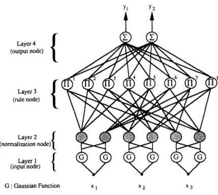
In this subsection, we will construct a four-layer N F N N structure to implement the fuzzy inference system stated in (2). We first denote by Aij the membership function of the jth term node of input variable xi and assume that xi has n~ term nodes for fuzzy partition. An N F N N structure with three input variables, two term nodes for each input variable, two output nodes, and eight rule nodes is illustrated in Fig. 1.
Yl Y2 Layer 4 / (output node) ( Layer 3 / (rule node) ( Layer 2 / (normalization node)( Layer 1 (input node) t
C.-T. Chao, C.-C. Teng / Fuzzy Sets and Systems 75 (1995) 17-31 19
G : Gaussian Function x 1 x 2 x 3
Fig. 1. The structure of the NFNN.
L a y e r 1." linguistic term layer
This layer uses a Gaussian function as a membership function, so the output of the jth term node associated with x~ is
#A.(X,) = exp( -- (x' -- m'J'~2"],
\ a~i / / (3)
where mij and tr~j denote the mean (center) and variance (width) of A~j, respectively.
L a y e r 2." normalization layer
This layer performs a normalization procedure for the output of layer 1. Notice that no weight is adjusted here and that normalization has been done, i.e.,
' X ~lAo(Xi)
~A,,( i ) -
n,
~'k : 1 ~lAik(Xi) ' (4)
where ~t~(x~) denotes the normalized output of/~A,(X~). The normalization procedure can also be represented in another form,
uA{(xi)
(5)
~,~(x,)
E~'=~
~,~(x,)
2 0 C.-T. Chao, C.-C. Teng / Fuzzy Sets and Systems 75 (1995) 17-31
Layer 3." rule layer
This layer implements the links relating preconditions (normalized node) to consequences (output node). The connection criterion is that each rule node has only one antecedent link from a normalized node of a linguistic variable. Hence there are Iqi n~ rule nodes in the initial form of N F N N structure. We mention that there is still no weight adjustment in this layer. The output of the jth rule node is
out 3 = f i I~'A,~(X,), (6)
i = l
where k is determined by the connection criterion, or, in another form,
out~
= fi M~(xi).
(7)
i = I
Layer 4: output layer
All consequence links are fully connected to the output nodes and interpreted directly as the strength of the output action. This layer performs centroid defuzzification to obtain the numerical output:
j=l i=1
Thus, the overall net output is treated as a linear combination of the consequences of all rules instead of the complex composition of a rule of inference and the defuzzification process.
In the following, we will start from (8) and show that the output y of the N F N N system is equal to the output of the simplified fuzzy inference system stated in (2). To begin with, from the connection criterion between layers 2 and 3, we obtain the equation
i = 1 j = l j = l i = 1
Substituting (5) into (8), we have
Y = ~-, #~ ~tA~(Xi) _ Z j=l BJ(H~: 1 laA~(Xi)) (I0)
n ~ - - - - n nl
i = 1 E k = l ['lAik(Xi) Hi= 1 2 k = 1 ]~Ait,(Xi)
Applying (9) to the denominator of the above equation, we can obtain the same result as in (2). This means that the proposed N F N N structure is equivalent to the simplified fuzzy inference system.
2.2. Supervised learning
The adjustment of the parameters in the proposed N F N N can be divided into two tasks, corresponding to the IF (premise) part and T H E N (consequence) part of the fuzzy logical rules. In the premise part, we need to initialize the center and width for Gaussian functions. To determine these initial terms, a self-organization- map (SOM) [11] and fuzzy-c-means (FCM) [-15] are commonly used. Another simple and intuitive method of doing this is to use normal fuzzy sets to fully cover the input space. Since the final performance will depend mainly on supervised learning, we choose normal fuzzy sets in this paper. In the consequence part, the parameters are output singletons. These singletons are initialized with small random values, as in a pure neural network.
C.-T. Chao, C-C. Teng / Fuzzy Sets and Systems 75 (1995) 17-31 21
A gradient-descent-based BP algorithm [14] is employed to adjust N F N N ' s parameters. The goal is to minimize the error function
E = ½ ( d - y ) 2, (11)
where y is the output of the N F N N and d is the desired output for the ith input pattern. If w~j is the adjusted parameter, then the learning rule is
and
c3E
Wij(t ÷ 1 ) = Wij(t ) -- ~ ~ ÷ o~Awij(t)
uw~j
Awij(t) = wij(t) - wij(t - 1), (12)
where q is the learning rate and ct, 0 < ct < 1, is the momentum parameter.
Substituting (3)-(8) into (12), we obtain the back-propagated error signals 6 and the update rules for the NFNN: j4 = d - y, (13) 63 = 64fl j, (14) 3 3 , 6~(t) - 6~ o u t ~ , (15) p k = l q flJ(t + 1) = flJ(t) + rl6%ut 3 + ctAflJ(t), (16) 2(xi - mij)
mij(t + 1) = mij(t) + q6 2 tr-~ij + ~Amij(t), (17)
- r e , j ) 2
O'i)(t ÷
1) = tri~(t) + rlJ 2 2(xi a 3+ otAtrij(t),
(18)where the subscripts p and q in (15) denote, respectively, all the rule nodes connected to thejth term node and the kth term node of xl.
3. Rule combination
In general, a fuzzy neural system with more rules will take more parameters and will provide better performance. In fact, however, some of these rules are unnecessary or redundant. A rule elimination method is a method that eliminates unnecessary rules by simply abandoning rules with relatively small consequence weights. The purpose of a rule combination method, on the other hand, is (a) to eliminate redundant preconditions of fuzzy rules, and (b) to combine certain pairs of fuzzy logical rules into a single, logically equivalent rule. The reason rules can be combined is very clear. For example, ifa continuous function is of the form
f(xl,x2)
~ - X 2 / ( ( X 1 - - 4) 2 ÷X2),
then if xl = 4, we have f = 1 for all x2. Thus f i s not affected by x2 inthis case, and x2 is a redundant input when xl = 4.
In this section, we first introduce some basic definitions and concepts which will be helpful in deriving the sufficient condition for rule combination. We also provide a rule combination algorithm and give an example to clarify the main idea behind the proposed rule combination method.
22 C.-T. Chao, C.-C. Teng / Fuzzy Sets and Systems 75 (1995) 17 31
3.1. Definitions
Many definitions of logic expressions were introduced in [1] to provide a means for multilevel logic synthesis. In order to treat a mathematical equation as a logic expression, we also have to state some definitions, as follows. We refer interested readers to [1,4] for details.
A variable can be thought of as a literal (e.g., a or b), and a cube represents the conjunction of its literals (e.g., a, abc, and bcd).
An expression is a set of cubes. For example, y = abc + de + f g is an expression consisting of three cubes abc, de, and fg. We say an expression is cube-free if no cube divides the expression evenly (e.g., ab + d is cube-free but ab + ad is not, since ab + ad can be divided evenly by a cube a).
The primary divisors of an expression f are the set of expressions D ( f ) = { f / C [ C is a cube}.
For example, we may define an expression x as x = abe + bce + a c f + b c f
= e(ab + bc) + c ( f a + f b )
= be(a + c) + cf(a + b). (19)
Then ab + bc and fa + f b are the primary divisors of x and they are obtained by x/e and x/c, respectively. Also, a + c and a + b are the primary divisors of x.
The kernels of an expression f are the set of expressions K ( f ) = {gig ~ D ( f ) and g is cube-free}.
In other words, the kernels of an expression f are the cube-free primary divisors of f. The cube C used to obtain the kernel k = f / C is called the co-kernel of k. In (19), for example, a + c and a + b are kernels corresponding to co-kernels be and c f, respectively, since they are cube-free primary divisors of x. On the other hand, the primary divisors ab + bc and fa + f b are not kernels of x, because they are not cube-free. The kernels a + c and a + b are also called level-O kernels, which have no kernels except themselves. We will use the notation K ° ( f ) to represent the set of level-0 kernels of f.
Moreover, we define the literal o} as the output of the normalized node corresponding to t h e j t h term node of the ith variable xi and define the expression O i as follows:
n ,
0 i = 5" i ~.~ Oj = O' 1 -~- 0 2 3t- "'" "~ O n . i i (20)
j = l
Notice that, for brevity, we use ~ and [l to represent logical sum and logical product, respectively. Without loss of generality, we consider multi-input-single-output fuzzy inference systems, since a multi- output system can always be decomposed into a group of single-output systems. Let y* denote the partial summation of the final output y in (8) with the same consequence weight fl*. Then we have
y* = fl* o ,
j 1
where k is determined by the connection criterion between normalization nodes and rule nodes and m' is the number of rules with the same consequence weight fl*. When y* is divided by fl*, we define another
C-T. Chao, C-C Teng / Fuzzy Sets and Systems 75 (1995) 1~31
23
expressiony _ s a m e = y* / fl* = ~ flOCk,
j=li=l
where y _ s a m e is expressed in two-level sum-of-product form.
(21)
3.2. The rule combination theorem and algorithm
Now we are ready to establish the theorem to determine whether rules can be combined in the N F N N system.
Rule Combination Theorem. In the N F N N system, let 0 i and y _ s a m e be defined as in (20) and (21),
respectively, and let K ° ( y _ s a m e ) be the set o f level-O kernels o f y_same. I f there exists an Oi ~ K ° ( y _ s a m e ) , 1 <~ i ~ n, then some rules can be combined into a single equivalent rule.
Proof. If there exists an O i e K ° ( y _ s a m e ) , 1 <<. i <<. n, then the expression y _ s a m e can be represented in the form y _ s a m e = (co)*O i + s_o_p, where co is the co-kernel corresponding to O i and the term s_o_p is the algebraic quotient of y _ s a m e / c o in sum-of-product form. Since numerically O i is equal to unity, i.e.,
0 i--~- ~
~,Io(Xi)~--- ~
~Aij(Xi) - 1i=1 '
where we have applied (4), y_same can be simplified as y_same = co + s_o_p. This means that some rules can
be combined into a single equivalent rule. []
With slight modification, the theorem stated above can also be extended to an M I M O system. The
theorem tells us that instead of finding all the kernel sets we just need to check whether the expression y _ s a m e
has level-0 kernel O( In practical application, we can repeatedly apply this theorem until no rules can be combined. An algorithm for rule combination is stated below.
Rule Combination Algorithm
Let the expression y _ s a m e be in sum-of-product form.
c h e c k = Y E S / * Y E S - - - - 1 N O = = 0 * /
tempi -- O for i = l t o n
W H I L E ( c h e c k )
{
F O R i = 1 T O n
IF literal o~ appears in at least one cube of y_same for j -- 1 to ni
W H I L E ( f i n d ( i ) )
{
C = Z"k'= * (cubek)
i has the same quotient q for j = 1 to n; IF cubej divided by literal o i
{
y _ s a m e = y _ s a m e -- C + q tempi = 1
} }
24 C.-T. Chao, C - C . Teng / Fuzzy Sets and Systems 75 (1995) l ~ 3 1 IF t e m p i = = O f o r i = 1 t o n check = N O ELSE check = YES tempi = 0 for i = 1 to n
}
find(i){
IF we can find a "new" set of ni cubes, denoted by cubej ( j = 1 to ni), from y_same such that the cubej has literal o~ for j = 1 to ni
return YES
ELSE return N O
}
The inner while loop of the algorithm checks whether O i is the kernel of y_same; if it is, then y_same can be
simplified. Since a kernel m a y have at least one corresponding co-kernel, we need the inner while loop. Moreover, the function find ( ) finds a new candidate C, which is several cubes in sum-of-product form, from y_same. Suppose C can be factored as a product of O i and a cube q; then we replace C by q in the expression y_same. To ensure that O i is not a kernel of y_same, we have the outer while loop in the algorithm.
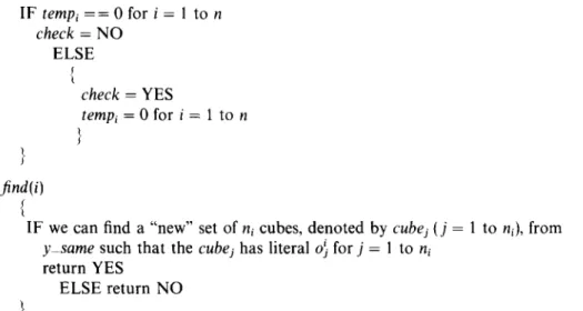
Fig. 2 presents an example to illustrate the proposed algorithm. The rules of the original N F N N system with the same consequence weight are shown in Fig. 2(a). Then we have
1 2 3 1 2 3 1 2 3 1 2 3 1 2 3 1 2 3 1 2 3 (22) y _ s a m e ~ 0 1 0 1 0 1 -~ 0 1 0 1 0 2 -+- 0 1 0 2 0 1 + 0 2 0 1 0 2 --[- 0 3 0 1 0 1 + 0 3 0 1 0 2 + 0 3 0 2 0 1 .
We apply the rule combination algorithm first to check whether 01 = o~ + oI + oI is the kernel of y_same. The answer is "yes", and y_same becomes
= O 1 0 2 ( O 1 -+- 0 1 0 1 0 l q- 0 1 0 2 0 1 q- 0 3 0 1 0 1 + 0 3 0 2 0 1
y_same 2 3 1 0 1 d - 0 1 ) + 1 2 3 1 2 3 1 2 3 1 2 3
2 3 1 2 3 1 2 3 1 2 3 1 2 3 (23)
= O 1 0 2 ~- O 1 0 1 0 1 q- 0 1 0 2 0 1 -[- 0 3 0 1 0 1 -~- 0 3 0 2 0 1 .
Fig. 2(b) shows the result. Because 01 is no longer a kernel of the new y_same, we try 02 = o 2 + 02 and repeat the above procedure. Then we obtain
2 3 1 3 2 0 2 ) -t- 0 3 0 1 0 1 ~- 0 3 0 2 0 1
y_same = 0102 + 0101(01 + 1 2 3 1 2 3
2 3 1 3 1 2 3 1 2 3 (24)
-~- O 1 0 2 -~- O101 • 0 3 0 1 0 1 • 0 3 0 2 0 1 .
The resulting connection links in N F N N are shown in Fig. 2(c). We can still extract the kernel 0 2 from the above expression, thus
01o2 + 0101 + 0301(01 + o~)
y_same = 2 3 1 3 1 3 2
2 3 1 3 1 3
(25)
= O 1 0 2 + O101 -~ O301 ,
The result is illustrated in Fig. 2(d). Since the expression y_same never has the kernels O 2, 0 3, and O 1, we stop the procedure and can guarantee that no further rules can be combined.
In fact, the basic idea behind the theorem and algorithm stated above is similar to the three criteria for rule combination presented in 1-12]: (1) the rules to be combined into a single rule node must have exactly the same consequences, (2) some preconditions are c o m m o n to all these rules, and (3) the union of other
C.-T. Chao, C.-C. Teng / Fuzzy Sets and Systems 75 (1995) 17-31 25
y Y
normalization node ~ ~ ~ normalization
x 1 x 2 x 3 Xl x 2 x3
(a)
(b)
y rule node normalization node ~ Xl x 2 x 3(c)
y rule node normalization Xl x 2 x 3(d)
26 C.-T. Chao, C . - C Teng / Fuzzy Sets and Systems 75 (1995) 17-31
preconditions of these rule nodes constitutes the entire term set of some input linguistic variables. The difference between their rule combination method and ours is as follows. First, they apply rule combination before supervised learning, while we do it after supervised learning. Second, in their method the "same consequences" referred to in criterion (1) are still fuzzy terms while in our method they are singleton weights. Third, the rules they are combined in their method are just a subset of the rules with the same consequences. They do not provide an efficient method for finding the rules to be combined, while we do. Fourth, the specially designed N F N N provides a proof that all rules that can be combined have been found, whereas their method offers no such proof.
3.3. Minimization p r o b l e m in rule combination
Although the rule combination algorithm presented in the last subsection provides an intuitive and simple method for rule combination, it leaves an unsolved minimization problem. F o r example, the example in (22) has the final reduced form shown in (25) if we extract the kernels in the order O 1, 0 z, and 03. But if we extract the kernel 03 first, we will have
1 2 1 2 3 1 2 3 1 2 1 2 3
y _ s a m e = o101 + 010201 + 020102 + 03Ol + 030201, (26)
which can be reduced no further, This means that the proposed rule combination algorithm could be extended to solve the minimization problem by extracting the kernels in every possible order.
The expression of y _ s a m e in (21) is in fact a multiple-valued f u n c t i o n (mvi-function), whose input and output variables can take two or more values, y _ s a m e is an mvi-function that has n multiple-valued inputs and one binary-valued output. Moreover, each input has n~-valued logic representations. Thus, we refer the interested reader to [-13] for a discussion of multiple-valued minimization; Ref. [13] presents an extension of the original complementation algorithm of the program ESPRESSO [2] for binary-valued functions.
3.4. Co nsequence weights with the s a m e value
In the N F N N system, consequence weights with the same value will be iteratively found for rule combination. We have found in practical simulation results that rules seldom have exactly the same consequence weights without any approximation. In this subsection we propose a method for coping with this problem.
Consider all the existing consequence weights to be sorted in increasing order so that they form a sequence betai,~,, where iter is the number of iterations. Thus, we obtain
betal,e, = ( b l , b2 . . . bo~i,er)~, (27)
where 9(iter) is a function of iter. It is clear that g(1) = m for the initial m consequence weights. Furthermore, we denote by B,er,~ the set of successive r(iter) elements in beta,~,, where i = 1, 2 . . . 9(iter) - r(iter) + 1 and r(iter) is a function of iter that is set by the user at each iteration. That is,
B,~,., = {bl, b, +1, b, + z, ..., b, +,,,e,)_, }, (28)
we emphasize that b~ <<, b~+ 1 <~ "'" <~ bi+r~te,~- ~ is still satisfied. We define a difference measure ( D M ) for set B to represent the degree of difference between these elements in B:
O M i , e , i = D M ( B i , e r i) = Ibi+r(iter) 1 - bil (29)
• . Imedian(Bi,e~.i) I '
where median is a function that finds the median number of a set (if there are two medians in a set, take the average of the both medians as the output median). This means that the smaller the value of DMi,e,.~ is, the
C.-T. Chao, C.-C. Teng / Fuzzy Sets and Systems 75 (1995) 17-31 27 larger the degree of nearness for the r(iter) values in Bi, er, i. For example, the set { 1, 3, 5} will have a larger D M value then the set {2,3,4}, but the D M value of the set {0.1,0.2,0.3} is equal to that of the set {1,2,3}. Furthermore, the median function can be replaced by the average function, although the latter is more complicated. The user also has to set a parameter eb. If all the values of DMite,.i are greater than eb, there will be no elements in betaiter that are approximately equal. Thus at this iteration the N F N N system stops.
If DMiter,! = minvi OMiter, i ( o f course, DMiterd < e~ is satisfied), the consequence weights treated as the same in the N F N N system will be determined formally. Let V be the set of all these consequence weights of the form
Viter = {I) [ 1) C-- betai,er and Iv - median(Biter, t)[ ~< [median(Biter, l)[* T B% }, (30)
(b)
S
(c)
28 C.-T. Chao, C.-C. Teng / Fuzzy Sets and Systems 75 (1995) 17 31
where T B % is the tolerance bound set by the user. Since at least mini = x ... ni consequence weights must be the same for possible rule combination, the n u m b e r of elements in V, er must be greater than mini= ~ ... ni.
Once the set
Vite,
is obtained, we can construct the expressiony_same
and proceed to do rule combination.When several rules are combined into an equivalent one, the combined consequence weights will be deleted
from
beta,e,.
A new equivalent consequence weight, the average of these combined consequence weights, willbe added in
betai,er
to replace the respective combined consequence weights. Therefore, we construct a newbetaiter
for the next iteration. On the contrary, if no rules are combined thatbetaite,, DM,~,,I,
andViter
will be unchanged in the next iteration. In such cases, theDMiterd
in the next iteration is redefined as the leastDM,er,i
that is not yet chosen in the former iterations. In fact, the simulation results in the next section indicate that this method if highly efficient.4. Numerical example
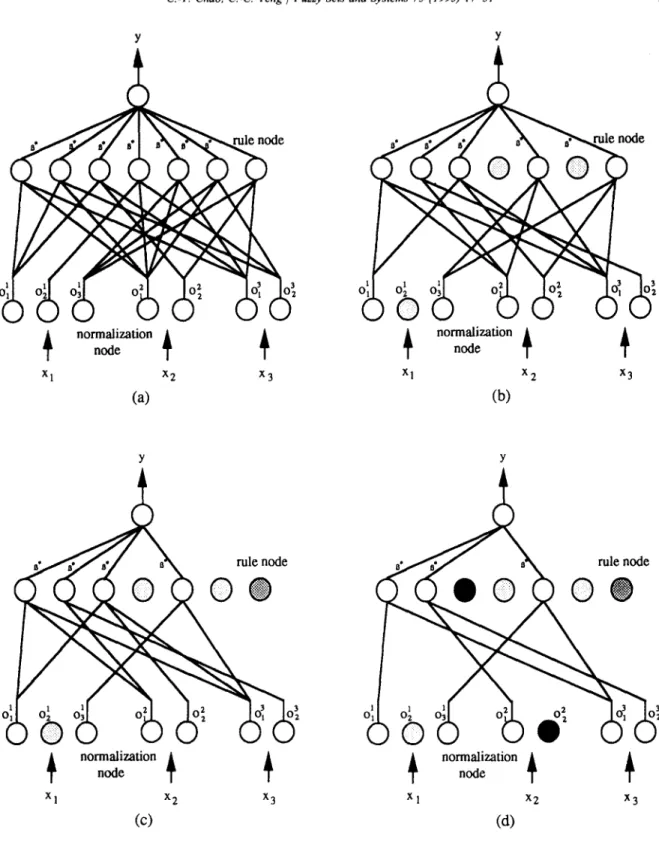
The following example of a continuous function is presented to illustrate the proposed procedure for rule combination:
sin(nx2)
f ( X l , X 2 ) -- for - 1 ~< Xa ~< 1 and 0 ~< x 2 ~ 1. 2 + sin(rtxl)
The initial structure of the N F N N uses seven term nodes for x~ and five for x2, i.e., in this case we have 7 x 5 initial rules. Since the optimal choice of the n u m b e r of term nodes is still a difficult problem, we tried several cases and found that the case of 7 × 5 initial rules is acceptable. Suppose one epoch of learning takes 247 time points, The supervised learning is continued for 300 epochs of training and the sum of squared error is c o m p u t e d for each epoch of learning as
24-7
s s E = ~ ( y l k ) - ~ / k ) ) 2
k = l
The desired i n p u t - o u t p u t relation of f i s shown in Fig. 3(a). The fuzzy sets for these linguistic term nodes are normally and uniformly initialized. We choose q = 0.01 and a = 0.9 for supervised learning. The parameters
Table 1
Initial and final parameters of the membership functions
Term sets Initial parameters Final parameters
Mean Variance Mean Variance
A l 1 -- 1.000 0.127 -- 0.695 0.584 A12 - 0.667 0.127 -- 0.493 0.310 Ai3 -- 0.333 0.127 0.013 0.804 A14 -- 0.000 0.127 0.064 0.004 A15 0.333 0.127 0.378 0.003 A16 0.667 0.127 1.018 0.098 A17 1.000 0.127 1.133 0.017 A 21 0.000 0.095 0.021 0.199 A22 0.250 0.095 0.193 0.174 A23 0.500 0.095 0.566 0.219 A24 0.750 0.095 0.819 0.159 A25 1.000 0.095 1.014 0.162
C-T. Chao, C-C Teng / Fuzzy Sets and Systems 75 (1995) 17-31 29
Table 2
The final rules after supervised learning
Table 3
The final rules after rule combination
Preconditions Consequence Preconditions Consequence
1 Atl, Azt -0.119 2 AI2, A21 -0.534 3 AI3, A21 -0.090 4 At4 , A21 0.710 5 Als, A21 0.481 6 Al6, A21 -- 0.151 7 AIr, A21 0.812 8 A11, A22 0.379 9 AI2, A22 1.806 l0 hi3 , A22 0.356 11 A14, A22 0.704 12 Ats, A22 0.609 13 AI6, A22 0.506 14 ArT, A22 0.868 15 All, A23 0.385 16 At2, A23 1.924 17 A13, A23 0.396 18 A14 , A23 0.755 19 Als, A23 0.548 20 A16, A23 0.531 21 A17, A23 0.893 22 AI l, A24 0.236 23 AI2, A24 1.139 24 At3 , A24 0.221 25 At,,, -4.24 0.881 26 Al5, A2,, 0.584 27 A16, A2,, 0.317 28 A17, A24 0.928 29 Air, A25 - 0 . 0 7 7 30 At2, A25 - 0.350 31 AI3, A25 - 0.064 32 AI,*, A25 0.890 33 Als, A25 0.610 34 A16, A2s - 0.090 35 A17, A2s 0.927 1 All, A21 -0.119 2 AI2, A21 -0.534 3 A I3, A21 - 0.090 4 At* 0.788 5 A15 0.566 6 Aio, A21 -0.151 7 Al7 0.886 8 A11. A22 0.379 9 A12, A22 1.806 10 A13, A22 0.356 11 A16, A22 0.506 12 Air, A23 0.385 13 At2, A23 1.924 14 At3, A23 0.396 15 Al6, A23 0.531 16 AI i, A24 0.236 17 AI2, A24 1.139 18 A13 , A24 0.221 19 A16 , A24 0.317 20 At 1, A25 - 0.077 21 AI2, A2s -- 0.350 22 AI3, A2s - 0.064 23 A16, A25 - 0.090
of the initial and final membership functions are illustrated in Table 1. The rules obtained after 300 epochs of learning are listed in Table 2 with performance represented by SSE = 0.069155 (mean square error is 0.000280).
To find the rules with the same consequence weights, we set r(-) = 5, eb = 0.3 and T B % = 20% for each iteration. Then we have rules 7, 14, 21, 28, and 35 in Table 2 to be combined in the first iteration. The resulting equivalent rule is rule 7 in Table 3. Rules 5, 12, 19, 26, and 33 in Table 2 are another set of rules that are combined in the fourth iteration. Finally, rules 4, l l , 18, 25, 32 in Table 2 are combined in the fifth iteration. The final rules after rule combination are listed in Table 3. The number of rules has been reduced from 35 to 23. Fig. 3(b) shows the performance surface of the function fafter rule combination. The SSE after rule combination is still equal to 0.069155, thus attesting to the feasibility of the proposed system. We also list the number of rules after rule combination under different tolerance bounds in Table 4.
30 C.-T. Chao, C.-C. Teng / Fuzzy Sets and Systems 75 (1995) 17 31
Table 4
The number of rules after rule combination under differ- ent tolerance bounds (r(-) = 5 and e b = 0.3)
Tolerance bound 5% 10% Number of rules 35 31 Sum of squared errors 0.069155 15% 20% 30% 27 23 23 Table 5
The final rules after rule elimination
Preconditions Consequence 1 AII, A21 - 0 . 1 1 9 2 At2, A21 - 0 . 5 3 4 3 At,* 0.788 4 A 15 0.566 5 AI6, A21 -0.151 6 A17 0.886 7 All, A22 0.379 8 AI2, A22 1.806 9 A13, A22 0.356 10 Al6, A22 0.506 11 Atl, A23 0.385 12 A12, A23 1.924 13 Al3, A23 0.396 14 A16, A23 0.531 15 All, A24 0.236 16 AI2, A24 1.139 17 A13, A2,* 0.221 18 A16, A24 0.317 19 AI2, A25 - 0 . 3 5 0
We can also use the rule elimination method to eliminate these rules which are less important, i.e., to eliminate rules with small consequence weights compared with other rules. Hence rules 3, 20, 22, and 23 in Table 3 can be eliminated. Table 5 lists the final 19 rules, and the corresponding performance surface with
SSE --- 0.238726 (mean square error is 0.000967) is shown in Fig. 3(c). 5. Conclusion
In this paper we have explored a procedure for rule combination in an N F N N system. The structure of the proposed N F N N makes the rule combination method efficient and effective. A sufficient condition for rule combination in the N F N N system is derived and an algorithm for performing rule combination is provided. The sufficient condition and the algorithm can be extended to M I M O systems with a slight modification. Simulation results show that when combined with a rule elimination method the rule combination method can greatly reduce the number of rules.
References
I-1] R.K. Brayton, R. Rudell, A. Sangiovanni-Vincentelli and A.R. Wang, MIS: a multiple-level logic optimization system, IEEE Trans. CAD 6(6) (1987) 1062-1081.
[2] R. Brayton, G. Hachtel, C. McMullen and A. Sangiovanni-Vincentelli, Logic Minimization Algorithms.for VLSI Synthesis (Kluwer Academic Publishers, Boston, MA, 1984).
[3] J.J. Buckley and Y. Hayashi, Can fuzzy neural nets approximate continuous fuzzy functions?, Fuzzy Sets and Systems 61 (1994) 43-51.
[4] G. De Micheli, Synthesis and Optimization of Digital Circuits (McGraw-Hill, New York, 1994).
[5] B.W. Grant and A.V. Wal, The use of neural networks for automation of fuzzy knowledge base creation, 1st Asian Fuzzy Systems Syrup., Singapore (1993) 340-345.
C-T. Chao, C-C. Teng / Fuzzy Sets and Systems 75 (1995) 17-31 31
[6] M.M. Gupta and D.H. Rao, On the principles of fuzzy neural networks, Fuzzy Sets and Systems 61 (1994) 1-18.
[7] S. Horikawa, T. Furuhashi, S. Okuma and Y. Uchikawa, A fuzzy controller using a neural network and its capability to learn expert's control rules, Proc. Internat. Conf. on Fuzzy looic and Neural Networks, July, lizuka, Japan (1990) 103-106.
[8] S. Horikawa, T. Furuhashi and Y. Uchikawa, On fuzzy modelling using fuzzy neural networks with the back-propagation algorithm, IEEE Trans. Neural Networks 3(5) (1992) 801 806.
[9] J.S. Jang, ANFIS: adaptive-network-based fuzzy inference system, IEEE Trans. Systems Man Cybernet. 23(3) (1993) 665-684. [10] C.C. Jou, On the mapping capability of fuzzy inference systems, Proc. lnternat. Joint. Conf. on Neural Networks, Baltimore, M L
(1992) 708-713.
[11] T. Kohonon, The self-organizing map, Proc. IEEE 78(9) (1990) 1461 1480.
[12] C.T. Lin and C.S.G. Lee, Neural-network-based fuzzy logic control and decision system, IEEE Trans. Comput. 40(12) (1991) 1320-1336.
[13] R. Rudell and A. Sangiovanni-Vincentelli, Multiple-valued minimization for PLA optimization, IEEE Trans. CAD/ICAS 6(5) (1987) 727 750.
[14] D.E. Rumelhart and J.L. McClelland (Eds.), Parallel Distributed Processing, Vol. I (M1T Press, Cambridge, MA, 1986). [15] M. Sugeno and T. Yasukawa, A fuzzy-logical-based approach to qualitative modeling, 1EEE Trans. on Fuzzy Systems 1(1) (1993)
7-31.
[16] L.X. Wang, Adaptive fuzzy systems and control (Prentice-Hall, Englewood Cliffs, N J, 1994).
[17] C.W. Xu and Y.Z. Lu, Fuzzy modeling identification and self-learning for dynamical systems, IEEE Trans. Systems Man Cybernet. 17(4) (1987) 683-689.