兩段式非線性回音消除之收斂性分析與最佳步伐調適

國 立 交 通 大 學

電信工程學系

碩 士 論 文

兩段式非線性回音消除之收斂性分析

與最佳步伐調適

Two-Staged Nonlinear Acoustic Echo

Cancellation: Convergence Analysis

and Step-size Control

研 究 生： 李克強

指導教授： 謝世福 博士

兩段式非線性回音消除之收斂性分析

與最佳步伐調適

學生：李克強 指導教授：謝世福

國立交通大學電信工程學系碩士班

摘要

免持聽筒或是視訊會議系統常驅動功率放大器和喇叭操作在飽和非線性 區，導致一般使用的線性回音消除器性能降低。在本篇論文中，我們將對非線性 回音消除建構出一個無記憶式片段線性(PWL)處理器串聯一個線性濾波器的模 型，它能有效降低運算量。另外，為了克服在串聯式系統的發散問題，我們採取 兩段式調適的方式，首先只有線性濾波器開始更新，接著PWL 和線性濾波器的 係數同時進行調適。更進一步，推導出它的收斂分析及穩定條件，並在電腦模擬 得到驗證。最後，我們發展出LMS 演算法在不同時間、不同時間及不同閥(tap) 的最佳步伐調適來加強收斂速度，同時提供他們實用的實現方式和電腦模擬。

Two-Staged Nonlinear Acoustic Echo

Cancellation: Convergence Analysis

and Step-size Control

Student : K. C. Li Advisor : S. F. Hsieh

Department of Communication Engineering

National Chiao Tung University

Abstract

Hand-free phone or teleconferencing system drives the power-amplification and loudspeaker commonly into saturated nonlinear region, leading to that the performance of conventional acoustic echo cancellation (AEC) reduced. In this thesis, we will build a cascade model which consists of a memoryless piece-wise linear (PWL) processor and a linear filter for AEC. It is beneficial to reduce the computation. Besides, in order to overcome the divergence problem in a cascade system, we will adopt the two-stage adaptation that starts with a linear filter, and then joint adaptation of PWL and linear coefficients follows. Further, the convergence analysis and stability criterion will be derived and the computer simulation will justify our analysis. Finally, LMS algorithms with optimum time-variant and time-&tap- variant step-sizes are developed to improve convergence rate. Their practical implementations and computer simulations are also provided.

Acknowledgments

In the process of writing this thesis, I received a lot of assistance and encouragement from many persons. First of all, I would like to express my profound gratitude to my thesis advisor Dr. S.F. Hsieh. Throughout the composition of this thesis, Dr. Hsieh provided me with many enlightening viewpoints and insightful suggestions. My special thanks go to all my lab-mates for their inspiration and help. Finally, Last but not least, I owe my deep appreciation to my family and my girlfriend for their endless support and encouragement.

Contents

中文摘要……….……….i

English Abstract

………ii

Acknowledgement

………..……….………iii

Contents……….……….iv

List of Figures

……….……….vii

List of Tables

……….………xii

1 Introduction

……….………1

2 Adaptive

Nonlinear

AEC

……….………6

2.1 Adaptive nonlinear LMS AEC using PWL structure………...6

2.2 Computation of adaptive nonlinear LMS AEC………..11

2.3 Partial update of adaptive nonlinear LMS AEC……….13

2.3.1 Periodic partial update LMS algorithm………...………14

2.3.2 Sequential partial update LMS algorithm………...………14

2.3.3 Stochastic partial update LMS algorithm………15

2.3.4 Variant-period partial update LMS algorithm……….………16

2.3.5 Located partial update LMS algorithm…….………..………17

2.4 Summary……….……….……….……….18

3 Two-staged adaptation and its convergence analysis

……….19

3.1 Two-staged adaptation………19

3.2 Convergence and stability analysis of linear adaptation………22

3.2.1 Mean bias of linear coefficient weight error………...22

3.3 Convergence analysis of joint adaptation of linear and PWL coefficients....29

3.4 Summary………..………..32

4 Step-size control for Nonlinear AEC

…………..………..…..33

4.1 Derivation of optimum time- variant step-size LMS (OTLMS) algorithm…34 4.2 Practical implementations of OTLMS algorithm………...36

4.3 Derivation of optimum time-&tap-variant step-size LMS (OTTLMS) algorithm………39

4.4 Practical implementation of OTTLMS algorithm………..43

4.5 Optimal step-size of NLMS algorithm………...45

4.6 Summary………46

5 Computer Simulations

………47

5.1 Simulation parameters and system performance measures………47

5.2 Nonlinear AEC based on LMS algorithm………..51

5.2.1 Performance comparison of PWL, polynomial and linear AECs……51

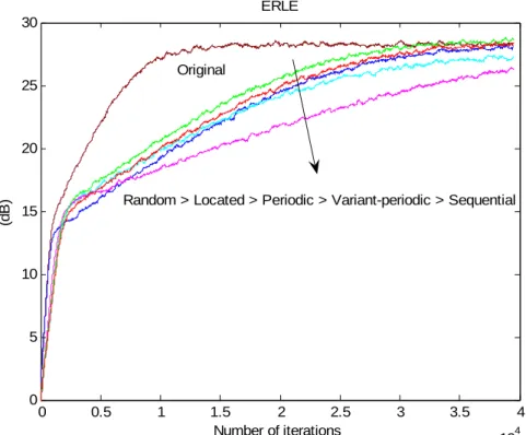
5.2.2 Comparison of partial update LMS algorithms……….……..56

5.2.3 Partition number of PWL processor………59

5.3 Two-staged adaptation and its convergence analysis……….61

5.3.1 Convergence and stability analysis of the first stage………...61

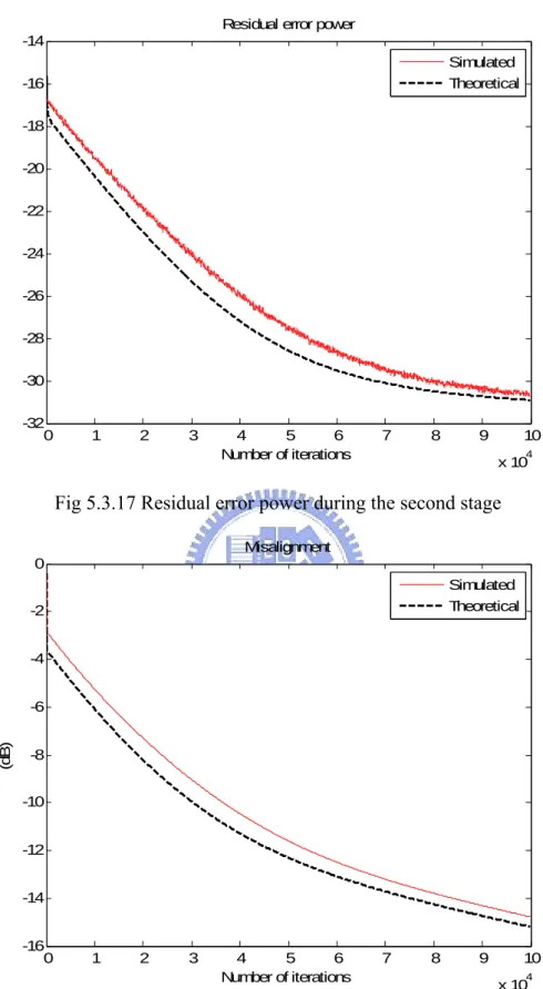
5.3.2 Convergence analysis of the second stage………..71

5.3.3 Switching point of two-staged adaptation………..….75

5.3.4 Experiments of the two-staged adaptation………..77

5.4 Control of step-size………81

5.4.5 OTLMS and OTTLMS algorithms in the two-staged adaptation.…..96

5.4.6 Experiments on the step-size controls……….98

6 Conclusion

……….……..104

Appendix

………...110

List of Figures

1.1 Diagram of hands-free telephone system………...………..1

1.2 Nonlinear acoustic echo cancellation system...………...……….2

2.1 Nonlinear acoustic echo canceller based on piecewise linear structure…..…7

2.2 (a) A CPWL curve with three segments (b)~(d) Associated canonical curves………..………...………..……….8

2.3 The block diagram of a PWL processor………….……...………..………..9

3.1 Cascade model of system (right hand part) and mirror adaptive system (left hand part)………...……...……….….….………20

3.2 Performance comparison of the two update schemes with two different step-sizes………..………..……….21

4.1 True nonlinear I/O mapping curve (solid), CPWL function (dot)…………... 38

4.2 RIR decay envelop………....……….……….…….44

5.1.1 Typical nonlinear I/O mapping curve using a raised-cosine function...50

5.1.2 Room impulse response………...………..……….50

5.2.1 Nonlinear I/O mapping curve of PWL and polynomial models………..52

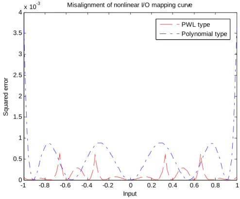
5.2.2 Modeling errors of PWL and polynomial models in fitting to a raised cosine function……….………….………...53

5.2.3 Modeling errors of PWL and orthogonal polynomial models in fitting a raised-cosine function………...………53

5.2.7 Saturated curve for nonlinear I/O mapping………..………57 5.2.8 ERLE of partial update schemes for a raised-cosine mapping……….58 5.2.9 ERLE of partial update schemes for a saturated mapping………...58 5.2.10 Raised cosine curve and the corresponding PWL curves with two partition

number: 2(b) and 4(c)…….………..59 5.2.11 ERLE for raised-cosine mapping using various partition numbers………….60 5.2.12 ERLE under saturated curve using various partition numbers……….60 5.3.1 Residual error power during the first stage with μ =0.01h ……….62

5.3.2 Linear coefficients misalignment during the first stage with μ =0.01h ……...62

5.3.3 Diverged residual error power during the first stage with

over-sizedμ =0.013h ………..………63

5.3.4 Diverged linear coefficients misalignment during the first stage with over-sizedμ =0.013h ………63

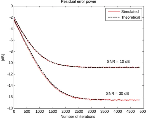
5.3.5 Linear coefficients misalignment during the first stage under different SNRs……….65 5.3.6 Residual error power during the first stage under different SNRs…………66 5.3.7 Linear coefficient misalignment during the first stage with different

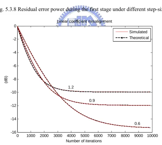
step-sizes………..66 5.3.8 Residual error power during the first stage under different step-sizes………67 5.3.9 Linear coefficients misalignment during the first stage with different powers of the output of PWL processor………67 5.3.10 Residual error power during the first stage with different powers of the output of PWL processor……….68 5.3.11 Linear coefficient misalignment during the first stage using different γ_d…..68 5.3.12 Residual error power during the first stage using different γd………69 5.3.13 Different Pdfs of the PWL processor output………69

5.3.14 Linear coefficients misalignment during the first stage using different Pdfs...70 5.3.15 Residual error power during the first stage using different Pdfs………70 5.3.16 Misalignment of combined coefficient weight error during the second stage.72 5.3.17 Residual error power during the second stage………..73 5.3.18 Misalignment of combined coefficient weight error under skipping during the 2nd stage……….73 5.3.19 Residual error power under skipping during the second stage………74 5.3.20 Misalignment of combined coefficient weight error under decoupling during the 2nd stage………74 5.3.21 Residual error power under decoupling during 2nd stage……….75 5.3.22 Misalignment of combined coefficient weight error of the two-staged adaptation………76 5.3.23 Residual error power of the two-staged adaptation………..76 5.3.24 Residual error power with different switching points………77 5.3.25 ERLE with a two level speech for linear AEC (dash line), nonlinear AEC based on PWL structure (solid line) and Polynomial one (dot line)…………78 5.3.26 ERLE with the speech of a woman with tone in mandarin………80 5.3.27 ERLE with the speech of a man with tone in English………80 5.4.1 Step-size of OTLMS algorithm………....82 5.4.2 Performance comparison between optimal time-variant and fixed step sizes..82 5.4.3 Nonlinear I/O mapping curves with the modeling……….84 5.4.4 Time-variant step-size with different mapping curves……….85 5.4.5 Residual error power with different mapping curves…...………85

5.4.8 Time-variant step-size using the first by using first-order recursive procedure with different β………...88 5.4.9 Residual error power using the first by using first-order recursive procedure with different β……….……….88 5.4.10 Residual error power using the two different procedures with βo…………89 5.4.11 Residual error power using the two different procedures with one-half β_o89 5.4.12 Residual error power using the two different procedures with two times βo.90 5.4.13 Performance comparison of convergence rate for OTLMS, OTTLMS and

fixed step-sizes……….91 5.4.14 Performance comparison of convergence rate for OTLMS, OTTLMS with three different mapping curves………..……….93 5.4.15 Model of RIR as an exponential decay envelope………93 5.4.16 Performance comparison of convergence rate for OTLMS and OTTLMS with three different mapping curves……….………94 5.4.17 Performance comparison of convergence rate for OTLMS and OTTLMS at

0.96 h

γ = with three different mapping curve….………94 5.4.18 Performance comparison of convergence rate for OTLMS and OTTLMS at

0.98 h

γ = with three different mapping curve……….………95 5.4.19 Performance comparison of convergence rate for OTLMS and OTTLMS at

0.94 h

γ = with three different mapping curve………95 5.4.20 Residual error power of OTTLMS, OTLMS, fixed step-size LMS for the

two-staged adaptation with fixed switching point……….97 5.4.21 Residual error power of OTTLMS, OTLMS, fixed step-size LMS for the two-staged adaptation with detection of state-stay linear filter………..97 5.4.22 ERLE of practical OTTLMS, practical OTLMS, fixed step-size LMS

5.4.24 ERLE of practical OTTLMS, practical OTLMS, fixed step-size LMS algorithm with the second part of speech and a pseudo nonlinear echo……100 5.4.25 Step-size of practical OTLMS algorithm with the second part of speech and a pseudo nonlinear echo………100 5.4.26 ERLE of practical OTLMS, fixed step-size LMS algorithm with the first part of speech and a true nonlinear echo………..……….101 5.4.27 Step-size of practical OTLMS algorithm with the first part of speech and a true nonlinear echo………102 5.4.28 ERLE of practical OTLMS, fixed step-size LMS algorithm with second part of

speech for true nonlinear echo………102 5.4.29 Step-size of practical OTLMS algorithm with the second part of speech for a true nonlinear echo………...………..103

List of Tables

Table 2.1 Look-up table of a PWL processor………...10 Table 2.2 Look-up table of decomposition introduced by Heredia [20]…………10 Table 2.3 Comparison of computational cost, no. multiplication per sample……..12

Chapter 1

Introduction

In these years, hands-free telephone and teleconference systems are widely used. Acoustic echo cancellation (AEC) is a major concern in telecommunications, where echo delay is particularly annoying for speakers. The problem occurs as a result of the reflections of the signal from the loudspeaker back to the microphone. We will introduce the fundamental problem and techniques of acoustic echo cancellation as follows.

Fig. 1.1 Diagram of hands-free telephone system

A simplified diagram of hands-free telephone system is shown in Fig. 1.1. Assume that a talker in the far-end uses microphone to communicate to the listener in near-end, the far-end speech will be transmitted back to the far-end through the loudspeaker and room impulse response. The main object of acoustic echo

In the past, based on the gradient theory, the acoustic echo that is linearly dependent on the loudspeaker can be cancelled effectively [1]-[3]. However, more and more telecommunications areas use heads-free devices to improve customer comfort. These devices drive higher power-amplification and power loudspeaker commonly driven into saturation region [4]. This issue leads to a nonlinear filtering problem that cannot be solved by conventional linear AEC.

In this thesis, the nonlinear AEC system is shown in Fig.1.2. The signal from the far end is passing through the nonlinear loudspeaker and the room impulse response and then is picked up by the microphone. The nonlinear AEC is supposed to cancel the nonlinear echo. The nonlinear echo can be cancelled perfectly if the nonlinear AEC filter is identical to the nonlinear loudspeaker and room impulse response.

( ) echo d n ( ) d n ( ) d n

Fig.1.2 Nonlinear acoustic echo cancellation system

The design and analysis of nonlinear adaptive filtering is difficult. The popular method is via polynomial functions, i.e. truncated Volterra [5], Wiener [6] and Hammerstein models [7]-[9]. Wiener and Hammerstein model are special cases of Volterra one with worse fitting but much less coefficients accompanied less

computations. Although Hammerstein model has the least complexity, it still has large computations.

In the thesis, we will employ the piecewise linear (PWL) [10] method to lessen this issue in nonlinear AEC. These are also other reasons which suggest that it may be worthwhile to investigate the simplicity of PWL implementation, as well as its theoretical analysis. The former is due to the fact that digital controllers based on such systems can be built easily using “if p(x) then f(x) else… ”. The latter own itself to the maturity of linear algebra.

Historically, a closed form of the canonical PWL (CPWL) was presented by Chua [10]. Lin used the least-mean-square (LMS) algorithm for CPWL [11]. The identification of Hammerstein model using two-segment nonlinearity, different polynomial functions on positive and negative regions, was demonstrated in [12]. Later on, Vörös demonstrated multi-segment PWL characteristics, the same idea as CPWL, with recursive-least-square (RLS) [13] in a special case of, high SNR, a specific set of initials and parameters. In this thesis, we will employ it for nonlinear AEC in various cases and discuss.

Although the PWL processor has benefit on the computation, it still is proportional to the linear filter length M . In the past, many types of selective update schemes for the adaptive linear filter have been described in [14]-[16]. We will extend their concepts and take advantages of the particular PWL structure to develop PWL coefficient selective update schemes.

misalignment, which can lead to a perpetual oscillating system.

In order to overcome this difficulty, Guérin [7] points out that the linear filter has to adapt continuously so as to react to any change in the acoustic path, and the PWL filter must not adapt until the linear filter has sufficiently converged. The two-staged strategy starts with a linear filter and then joint adaptation of PWL and linear coefficients follows once the linear filter has sufficiently converged in the first stage. Moreover, in this thesis we will derive the theoretical convergence analysis and stability criterion of the two-staged algorithm.

Next, we will focus on the step-size. We know a large step size gives a faster convergence but also large small residual error power. Therefore, various methods employing varying step-size have be examined by the other researchers, including time-varying [17], tap-varying [18] or both time- & tap- varying [19]. We will use the convergence analysis of the first stage to develop the optimum time-variant and optimum time-&tap-variant step-size LMS algorithm.

In Chapter 2, we introduce our system model and its update scheme. In Chapter 3, a two staged algorithm is used and its performance analysis of a PWL structure is proved analytically. In Chapter 4 The optimal step size with a nonlinear modeling error is derived. Simulations support our works in Chapter 5 and conclusion will be given in Chapter 6.

The main efforts in this thesis are:

1. We introduce a PWL structure of adaptive nonlinear AEC with lower complexity and develop its joint LMS adaptive algorithm.

2. We develop five types of PWL coefficients selective update schemes

3. For joint LMS adaptive algorithm, we derive and verify convergence analyses of the two-staged adaptation with a stability condition of linear step-size during the

first stage.

4. Further, we discuss the convergence behavior during the first stage with different factors, nonlinear effect, power and Pdf. of the far-end signal, step-size and SNR. 5. Optimum time-variant and time-&tap- variant step-size LMS algorithm of linear

adaptive filter with a nonlinear modeling error are derived and verified. 6. The corresponding practical forms are also proposed and discussed.

Chapter 2

Nonlinear Adaptive filter

In Chapter 2 we will build a system model for nonlinear AEC and develop its adaptive algorithm. Moreover, we will discuss the issue of the computation cost. Further, five types of partial update schemes will be presented to reduce the computational load.

In Section 2.1, the nonlinear AEC is first introduced as a cascade of nonlinear processor and linear adaptive filter, where a PWL function is used to model the nonlinear loudspeaker. Moreover, we will develop the joint LMS-type algorithm to update both PWL and linear coefficients. In Section 2.2, the computation complexity of the PWL-based nonlinear adaptive filter is compared to that of polynomial-based model and linear AEC. In Section 2.3, several partial update schemes are proposed to further reduce the computation at the cost of degraded convergence rate.

2.1 Adaptive nonlinear LMS AEC using PWL structure

In order to separate the identification of the nonlinear loudspeaker parameters and the tracking of the linear acoustic path changes, Fig. 2.1 shows a typical cascade nonlinear AEC [8], also known as a Hammerstein model. The far end signal x n( ) is

fed into the PWL processor f(x) that approximates the nonlinear mapping function with one or more linear equations. It has been exploited to compensate for the effect of nonlinear echo.

The output s n( ) of the PWL processor passes through a linear filter to form a pseudo

nonlinear echo d nˆ( ). Here we assume the nonlinear distortion is caused only by the

PWL processor Linear FIR filter ( ) x n ( ) s n ( ) e n d n( ) ˆ( ) d n + − ( ) v n ( )n w ( )n h o h o w ( ) echo d n PWL processor Linear FIR filter ( ) x n ( ) s n ( ) e n d n( ) ˆ( ) d n + − ( ) v n ( )n w ( )n h o h o w ( ) echo d n

Fig. 2.1 Nonlinear acoustic echo canceller based on piecewise linear structure The PWL function f(x) for the speech input range [-1 1] is assumed to be symmetric and its prototype is given by:

1 1 2 2 2 1 2 2 3 1 1 1 1 1 , ( ) , ( ) ( ) ( ) , , N N N N N N N m x x m x m x f x m x m m x α α α α α α α ₋ α α ₋ α α α ₊ ⎧ ≤ < ⎪ − + ≤ < ⎪ = ⎨ ⎪ ⎪ _{− + − + ≤ <} ⎩ (2.1.1)

wherem and_j α_jaccount for the slope and partition parameters of the linear subregion,

respectively, with α₁=0 and α_N+1 = . 1

The prototype of PWL function in Eq. (2.1.1) consists of a series of linear subfunctions which are properly partitioned into subregions of the nonlinear curve. Here we adopt a canonical piece-wise linear (CPWL) function [10], which is an analytic formula with several absolute-value operators. Its memoryless form with zero offset is given by

functions and N is the CPWL tap order. Extending to the symmetrical function and associated to Eq. (2.1.1), we can get a modified form as follows

( )

1 ( ) N j j j f x w f x = =

∑

, (2.1.2) where

( )

1 1 2 2 j j j f x =⎛_⎜ x−α − x+α +x⎞_⎟ ⎝ ⎠ and w₁=m₁,w_i =(m_i−m_i−1), ∀ =i 2 ~N.

We use an example to demonstrate how the CPWL function works. Consider a 3-segment CPWL function in Fig. 2.2 with partition paramentsα₂ =0.4 and α₃=0.7 and slopes w1= ,1 w2 = −0.4 and w3= −0.6. In Fig. 2.2, we can observe it performs

canonically with every breakpointα_i.

-1 -0.5 0 0.5 1 -1 -0.5 0 0.5 1 -1 -0.5 0 0.5 1 -1 -0.5 0 0.5 1 -1 -0.5 0 0.5 1 -0.4 -0.2 0 0.2 0.4 -1 -0.5 0 0.5 1 -0.2 -0.1 0 0.1 0.2

Fig. 2.2 (a) A CPWL curve with three segments (b)~(d) Associated canonical curves From now on, all PWL functions are of canonical form. The block diagram of a PWL processor is shown in Fig. 2.3, where the far end signal is decomposed to N analytic signals on the block f , then multiplied by its associated coefficient _j w , _j

and finally all of them are synthesized together to approximate the nonlinearly

( ) f x w f x1 1( ) 2 2( ) w f x w f x3 3( ) ( )b ( )c ( )d ( )a

distorted loudspeaker output. Here the j-th output of the block f_j

( )

x will be null

when the far end signal x is smaller than the j-th partition area value. It will be

beneficial to reduce computation load, which will be dealt with later.

1

f

...

1

w

w

₂

w

_N

s

2

f

f

_N

x

1

f

...

1

w

w

₂

w

_N

s

2

f

f

_N

x

Fig. 2.3 The block diagram of a PWL processor

The overall nonlinear AEC can be represented as a vector form. The output of the nonlinear processor ( )s n is given by

T s=w f⋅ , (2.1.3) where [ ... 1 2 ] T N w w w = w and

( ) ( )

( )

1 2 [ ... ]T N f x f x f x = f

resembles a decomposition that maps real numbers into vectors using a set of predefined partition parameters

{

0, ,α₂ αN,1

}

. For example, if the inputx is

positive and negative elements. [20] has also proposed a similar decomposition shown in Table 2.2. But our modified CPWL function is an explicit equation to achieve the decomposition and our procedure can be easily extended to that, by g x₁

( )

= f x₁

( )

and g_j

( )

x = f_j

( )

x − f_j−1

( )

x ,∀ =j 2 ~N.

Table 2.1 Look-up table of a PWL processor

( )

j f x x ≥α_j x ≤α_j 0 x≥ x-αj 0 0 x< x+α_{j 0}

Table 2.2 Look-up table of decomposition introduced by Heredia [20]

( )

j g x x >α_j+1 x ∈(α α_j+1, _j) x ≤α_j 0 x≥ αj+1− αj x− αj 0 0 x< α αj− j+1 αj+x n( ) 0

After discussing the decomposition of the vector f , we now come back to focus on the system flow in Fig. 2.1. From Eq. (2.1.3), the delay tap form of PWL processor

[

]

( ) ( ) ( -1) ... ( - 1)T n = s n s n s n M + s can be expressed as ( )n = ( )n ⋅ s F w , (2.1.4) where ( )

[

( ) ( 1) ( 1)

]

T n = n n− n M− + F f f f (2.1.5)

is the delayed tap mapping matrix. Therefore, the nonlinear AEC output signald n( )

( ) T( ) d n =s n ⋅h, where [ 0 1 ... ]-1 T M h h h =

h represents the estimated coefficients vector of the linear FIR filter with M being the length of the filter. The estimated error is

( ) ( ) ( )

e n =d n −d n

( ) T( ) ( )

d n n v n

= −s ⋅ −h

If the coefficients vectors are updated with step size μ_h andμ_w, a joint LMS-type adaptive algorithm according to the gradient of the cost function, _{( )} 2_{( )} J n =e n , is given by (n+ =1) ( )n +μh ( )n ⋅ ( ) ( )n e n h h w F =h( )n +μ_hs( ) ( )n e n (2.1.6) ( 1) ( ) T( ) ( ) ( ). w n+ = n +μ n ⋅ n e n w w F h (2.1.7) Now that we have developed a nonlinear adaptive filter algorithm for a PWL structure in (2.1.6) and (2.1.7). Similarly, in case of a polynomial structure, we can simply modify the delayed tap mapping matrix ( )F n in Eq. (2.1.6) and (2.1.7) by

setting it as follows: 2 2 2 ( ) ( 1) ( 1) ( ) ( 1) ( 1) ( ) ( ) ( 1) ( 1) N N N x n x n x n M x n x n x n M n x n x n x n M − − + ⎡ ⎤ ⎢ _{− − +} ⎥ ⎢ ⎥ = ⎢ ⎥ ⎢ _{− − +} ⎥ ⎣ ⎦ F .

2.2 Computation of adaptive nonlinear LMS AEC

The following discussion with respect to computational complexity is based on the number of real multiplications that is required by different structures. In Eq. (2.1.6), the matrix-vector product of ( )w ⋅F( ) is simply ( )s , which is readily

computation due to the matrix-vector product of T( ) ( )

n ⋅ n

F h in the vital equation (2.1.7). We note that the polynomial structure also has the same complexity [21].

We also note that the output of the operation f_j

( )

x in matrix F( )n would be

null when the far end signal x at iteration n is smaller than the partition

parameterα_j+1. Due to the zero output of the block f , the average number of _j

non-zero entries of ( )f n , the column vector of the matrix FT( )n , will be ( )

2

N O

for a uniformly distributed far end signalx. Besides, the computation cost will almost

reduces to ( ) 2

N

O M . The computational cost is listed in Table 2.3. We can see the

PWL structure has the lower computation than that of polynomial.

Table 2.3 Comparison of computational cost, no. multiplication per sample

Complexity of computation

No. of multiplication (approx.) per sample

Linear AEC 2M Polynomial NAEC (N =3) 2M MN+ PWL NAEC (N =3) 2 2 MN M +

2.3 Partial update of adaptive nonlinear LMS AEC

However, the PWL structure has reduced the computation on the matrix multiplication ( ) ( )T

n ⋅ n

F h with ( 1 ) 2

N

O + M multiplications. It still is proportional

to the linear filter length M . In acoustic echo cancellation, adaptive linear filter often require a large number M of coefficients to model the acoustic echo path with sufficient accuracy. It means that for long linear filter the adaptation task can become more prohibitively expensive.

Partial updating of the LMS adaptive linear filter has been proposed to reduce computational costs and power consumption [22], which is quite attractive in the area of mobile computing and communications that requires the adaptive linear filter to have a very large number of coefficients. Updating the entire coefficient vector of the adaptive linear filter is costly in terms of power, memory, and computations and is sometimes impractical for mobile devices.

In the past, many types of selective update schemes for the adaptive linear filter have been described in [14]-[16]. In this section, after introducing these selective update schemes, we will extend their concepts to the three types of PWL coefficient selective update schemes and take advantages of the particular PWL structure to develop the two types of ones in which only one PWL coefficient are adjusted at each sample time in order to reduce the matrix multiplication T( ) ( )

n ⋅ n

F h down to N multiplications.

2.3.1 Periodic partial update LMS algorithm

The most prevalent type in the literature of selective update scheme is referred to as the periodic LMS algorithm [14]. To reduce computation needed during the update part of the adaptive filter by a factor of N, the periodic LMS algorithm updates all the filter coefficients every N iterations instead of every iteration. In addition, the coefficient updates for this algorithm are regular, as only one coefficient is changed at one iteration. With this concept, the PWL coefficient update is given by

(

)

( ) ( ) ( ) ( ) , mod 1, / ( 1) ( ) ,otherwise. T j _j j j w n e l l l if j n N l N n N w n w n μ ⎧ + ⎡_⎣ ⋅ ⎤_⎦ = + = ⎢_⎣ ⎥_⎦ ⎪ + = ⎨ ⎪ ⎩ F h (2.3.1)

where ⎢ ⎥_{⎣ ⎦}⋅ denotes the truncation operation, n mod N denotes iteration n

moduloN. By considering N iterations of the updates in Eq. (2.3.1), it can be shown

that this algorithm is equivalent to the following N-fold coefficient vector update: ( ) ( ) ( ) T( ) ( )

n+N = n +μe n n ⋅ n

w w F h . (2.3.2) It describes a modified version of the LMS adaptive algorithm that uses every Nth instantaneous gradient to update the filter coefficients.

2.3.2 Sequential partial update LMS algorithm

Like the periodic LMS algorithm, for the sequential LMS algorithm [15] the update coefficient is chosen in a predetermined fashion, a regular pattern, but uses sequential gradient vector signal respect to w n . Extending to the PWL coefficients j( ) update, it is given by

(

)

( ) ( ) ( ) ( ) , if mod 1, ( 1) ( ) ,otherwise. T j _j j j w n e n n n j n N w n w n μ ⎧ + ⎡_⎣ ⋅ ⎤_⎦ = + ⎪ + = ⎨ ⎪ ⎩ F h (2.3.3)

Define Ψ by filling 1 on the j-th diagonal entry of the zero matrix and the above j update equation can be written in a more compact form

% 1

( 1) ( ) ( ) T( ) ( ). n N

n+ = n +μe n Ψ ₊ n ⋅ n

w w F h (2.3.4)

2.3.3 Stochastic partial update LMS algorithm

Being similar to the sequential LMS algorithm in the sense that also uses data-independent updating scheme, the stochastic partial update LMS [16] algorithm performs sequential instant gradient respect to w n . The difference is as follows. _j( ) At a given iteration k, the sequential LMS processes a regular processing strategy to select which one coefficient is to be updated, whereas for the stochastic partial update LMS, one of the coefficient is chosen at random from {1, 2 N} with probability1/ N and subsequently the update is performed i.e.,

( ) ( ) ( ) ( ) ,if is chosen at random ( 1) ( ) ,otherwise T j _j j j w n e n n n j w n w n μ ⎧ + ⎡_⎣ ⋅ ⎤_⎦ ⎪ + = ⎨ ⎪ ⎩ F h (2.3.5)

and the coefficient vector update can be expressed as ( 1) ( ) ( ) T( ) ( ),

n

n+ = n +μe nΨ n ⋅ n

w w F h (2.3.6)

where Ψ now is a random matrix chosen at random from n Ψj,j=1 N with

probability 1/ N (recall that Ψ by filling one on the j-th diagonal entry of the zero j matrix).

2.3.4 Variant-periodic partial update LMS algorithm

Unlike previous 3 well-known partial update schemes which are applicable to general LMS-type algorithms, we will take advantages of the particular PWL structure to develop a variant periodic partial update scheme.

As noted earlier, when the far end signal ( )x n is smaller than the partition

parameter α_j+1, the output of the operation f_j

(

x n( )

)

would be null. As a result, the

periodic LMS algorithm would be inefficient. In order to solve this issue, we propose a variant periodic LMS algorithm that takes advantages of the located partition area of far end signal ( )x n to avoid an inefficient update term.

For example, if the located partition area of far end signal ( )x n is the 2nd one,

the variant periodic LMS algorithm updates its first coefficient c n at time ₁( ) n and

second coefficient c n at time 2( ) n+1. If the located partition area of far end signal

( 2)

x n+ is the 3rd one, it updates the first coefficient c n at time ₁( ) n+2, second

coefficient c n at time 2( ) n+3 and third coefficient c n at time 3( ) n+4.Here we

denoted ( )Q n is the number of located partition area of far-end signal ( )x n at time

n. For example the partition is

{

0, 0.4, 0.7, 0.9, 1

}

and far end signal x n is 0.8, ( )

then ( )Q l is 3. The following non-period LMS algorithm is give by:

(

)

( ) ( ) ( ) ( ) , mod ( ) 1, ( ) / ( ) ( 1) ( ) ,otherwise T j _j j j w n e l l l if j n Q l l Q l n Q l w n w n μ ⎧ + ⎡_⎣ ⋅ ⎤_⎦ = + = ⎢_⎣ ⎥_⎦ ⎪ + = ⎨ ⎪ ⎩ F h (2.3.7) and the Q n -fold coefficient vector update can be expressed as ( )

( ( )) ( ) ( ) T( ) ( ), ( ) / ( )

n Q l+ = n +μe n n ⋅ n l=Q l ⎢_⎣n Q l ⎥_⎦

2.3.5 Located partial update LMS algorithm

Moreover, we will again utilize the particular PWL structure to develop a located partial update scheme.

As we know, the PWL processor would decompose the far end signal ( )x n into N analytic signals. The resulting analytic signal may be zero, depending on the far end

signal ( )x n . If far end signal ( )x n falls into the partition parameter α_j+1, the

corresponding j-th analytic signal will be null. This characteristic is also the main idea of the variant periodicLMS algorithm in Section 2.3.4. We also know the nonlinearity mostly happens for a high level input. Therefore, the (j+1)th entry of PWL coefficient vector has higher priority than the j-th entry.

By combining these characteristics, we propose a new partial update LMS algorithm, located LMS, for PWL coefficient as follows.

( ) ( ) ( ) ( ) , ( ) ( 1) ( ) ,otherwise. T j _j j j w n e n n n j Q n w n w n μ ⎧ + ⎡_⎣ ⋅ ⎤_⎦ = ⎪ + = ⎨ ⎪ ⎩ F h (2.3.9)

where ( )Q n is the number of located partition area of far end signal ( )x n at time

n. The update strategy is to choose the PWL coefficient which far end signal ( )x n

falls into. The benefit is when the power loudspeaker commonly driven with saturation region, mostly high level far end signal, the nonlinearity information is sufficiently used on the PWL coefficient. On the contrary, if the nonlinearity effect was insignificant in case of low level far end signal, it maintains the linear part of PWL coefficients. In the same way, the above update equation can be written in a more compact form as

partial update and full LMS algorithm.

2.4 Summary

In this chapter, we performed an adaptive nonlinear AEC based on a PWL type function and developed its joint LMS algorithm in section 2.1. Moreover, the comparison of computation complexity of three structures, linear AEC, nonlinear AEC in a case of PWL and polynomial one was discussed in section 2.2. The PWL one has the lower computation than that of polynomial and has just about 2M more multiplications than that of linear AEC. Finally, we presented 3 well-known and 2 proposed partial update of LMS algorithm in section 2.3. They all keep the computation on the matrix multiplication T( ) ( )

n ⋅ n

F h with M . The computation simulations in chapter 5 will compare the above performances explicitly.

Chapter 3

Two-Staged Adaptation and Its

Convergence Analysis

In Chapter 2, we have derived the joint adaptation of the nonlinear PWL AEC. However, each filter (or processor) behaves to compensate the other one’s misalignment. This can result in a perpetual oscillating system.

Therefore, in this chapter we will adopt two-staged strategy [7] to overcome this difficulty. This strategy is to start with a linear filter update in the first stage, and then joint update of both PWL and linear coefficients follows in the second stage.

In Section 4.1 the two-staged adaptation is introduced. In the first stage, the convergence analysis and stability criterion will be derived in Section 4.2. After that, we will derive the convergence analysis of the second stage in Section 4.3.

3.1 Two-staged adaptation

For simplicity, Fig. 2.1 is redrawn in Fig. 3.1. Here we assume the nonlinear loudspeaker and linear room impulse response are time-invariant; the near end signal

( )

v n only contains a white Gaussian noise (WGN) and the nonlinear echo

( ) T( ) ( )

o o

d n =s n ⋅h +v n ,

where ( )s n is the optimal PWL processor output with the optimal PWL coefficients _o

o

( ) x n ( ) s n ( ) e n d n( ) ˆ( ) d n + − ( ) v n ( )n w o h o w ( )n h ( ) o s n ( ) echo d n ( ) x n ( ) s n ( ) e n d n( ) ˆ( ) d n + − ( ) v n ( )n w o h o w ( )n h ( ) o s n ( ) echo d n

Fig. 3.1 Cascade model of system (right hand part) and mirror adaptive system (left hand part)

In the cascade structure of Fig. 3.1, if the joint updates of both nonlinear PWL coefficients ( )w n and linear coefficients ( )h n are performed simultaneously as

given in Eq. (2.1.6) and (2.1.7), the danger of divergence can happen. To illustrate this tendency of divergence, Fig. 3.2 includes two desperate divergent curves of joint-updating schemes with two step sizes μ_h =μ_w=0.002 and 0.003 and SNR=20dB.

The transient behavior of linear filter and PWL processor can account for the divergence problem encountered in cascade system. When both w( )n and ( )h n are

far away from their optimum coefficients w and _o h , respectively, in the early _o

transient stage, the resulting residual error ( )e n does not push either coefficients

towards their optimum points. As a result, convergence cannot be guaranteed, since each filter (linear filter or PWL processor) behaves to compensate the other one’s misalignment, which can lead to a perpetual oscillating system. An analytical stability criterion for joint adaptation of the nonlinear AEC can be very strenuous.

In order to overcome this difficulty, Guérin [5] points out that the linear filter has to adapt continuously so as to react to any change in the acoustic path, and the PWL filter must not adapt until the linear filter has sufficiently converged. The two-staged strategy starts with a linear filter, and then joint adaptation of PWL and linear coefficients follows once the linear filter has sufficiently converged in the first stage. Fig. 3.2 shows the significant improvements in residual error power using the two-staged algorithm.

In the past the convergence analysis of a cascade system was done under a perfect information linear or nonlinear part [21]. Next, we will proceed to derive the theoretical convergence analysis of the two-staged algorithm.

0 0.2 0.4 0.6 0.8 1 1.2 1.4 1.6 1.8 2 x 104 -22 -20 -18 -16 -14 -12 -10 -8 -6 -4 -2 Number of iterations Residual error power

Two-staged, μ=0.002

Two-staged, μ=0.003

Joint, μ=0.002 Joint, μ=0.003

Fig. 3.2 Performance comparison of the two update schemes with two different step-sizes

3.2 Convergence and stability analysis of linear adaptation

In the first stage, only linear coefficients update under a fixed PWL coefficients. We denote the linear filter weight-error vector by

( ) ( ) h n = n − o

ε h h . (3.2.1)

where h is the optimal linear filter. The estimation error produced by nonlinear o AEC filter can be expressed as

( ) ( ) ( ) e n =d n −d n T( ) ( ) T( ) ( ) o n o v n n n =s ⋅h + −s ⋅h

(

) (

)

_T( ) ( ) ( ) ( ) T ( ) o n o v n e n o n o h n =s ⋅h + − s +s h +ε ( ) T( ) T( ) ( ) e o v n n n n = −s ⋅h −s ⋅ε_h (3.2.2) where ( )se n =s( )n −so( )n is the error of PWL processor. Using Eq. (2.1.6) and (3.2.2), we may rewrite ε_h(n+1) as ( 1) ( ) ( ) ( ) h n+ = n +μh n e n − o ε h s h

(

)

( ) ( ) ( ) T( ) T( ) ( ) h n μh n v n e n o n n =ε + s −s ⋅h −s ⋅ε_h ( ) T( ) ( ) ( ) ( ) ( ) T( ) h n n h n h v n n n e n o μ μ ⎡ ⎤ ⎡ ⎤ =_⎣I− s ⋅s _⎦⋅ε + _⎣ s −s ⋅s ⋅h (3.2.3) _⎦

3.2.1 Mean bias of linear coefficient weight error

Taking the expectation on Eq. (3.2.3) and assuming the variation of εh( )n is slow compared with that of s( )n , the first moment of ε_h( )n is given by

{

_h( +1)

} (

_M - _{h s}

) {

_h( ) +E

}

{

_h( )

}

E ε n = I μ R ⋅E ε n f n , (3.2.4)

where ( ) ( ) ( ) ( ) ( )T h n =μh⎡⎣v n n − n ⋅ e n ⋅ o⎤⎦

f s s s h and R is the correlation matrix of _s

( )n

s by applying the unitary similarity transformation. We can diagonalize R s as follows: T

s s s = s

matrix consisting of the eigenvalues λ_{s i,} of R . Let _s ( ) T ( ), h n = s h n

k Q ε then we may transform Eq. (4.2.4) into the form

{

( 1)

}

(

)

{

( )

}

,e T h M h s h s s s o E k n+ = I −μ D ⋅E k n −Q R h , (3.2.5) where _, e s s

R is the cross-correlation matrix of ( )s n and ( )s_e n . We may go on to

express Eq. (4.2.5) as

{

}

1

(

1

)

, , ( ) (0) ( - ) e e T T n h s s s s o h s s s s o M h s E k n = −D Q R h− + k +D Q R h− I μ D . (3.2.6)

It makes sense that the linear coefficients weight error εh( )n convergences to a biased estimate due to the effect of nonlinear bias. This linear bias part also agrees with the optimal linear weight error [5], denoted by εh MMSE_, =hMMSE −ho, in the minimum mean square error (MMSE) sense. We will prove it as follows. First,

MMSE

h satisfies the equation { ( )} 0

MMSE

J n ₌

∇_{h h h} = , which depends on the correlation

matrix R_s and the cross-correlation matrix _,

e

s s

R . Using now the quasistationarity hypothesis, the optimal filter is then defined by the following expression

1 ,e

MMSE s s s o

−

= ⋅ ⋅

h R R h . Hence, it can yield 1

, ,e T h MMSE s s s s o − = − k D Q R h .

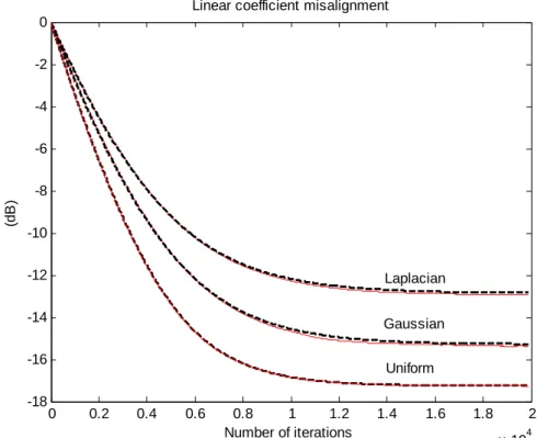
If the far end signal ( )x n is a white noise, we can find that the output of PWL

processor ( )s n is also white due to the symmetric PWL function. The white property

of ( )s n can be explained as follows. Applying the PWL function, we can rewrite the

correlation function of ( )s n as E s n s n

{

( ) ( +m)

}

=E f x n

{

(

( )

) (

f x n( +m)

)

}

. When n≠ , the expectation can be taken apart as m E f x n

{

(

( )

)

}

E f x n m

{

(

( + )

)

}

in case of

we have the matrix Q_s is an identity matrix, 2 s =σs R I and 2 ,e ,e s s =σs s R I, where 2 s

σ is the variance ofs n and( ) 2_,

e

s s

σ is the covariance of s( )n and ( )s_e n .

Now we may simplify Eq. (3.2.6) as

{

}

2

{

}

2 , ( +1) (1 ) ( ) . e h h s h h s s o E ε n = −μ σ E ε n −μ σ h (3.2.7)

We note that kh( )n is equal to εh( )n when the far-end signal is white. Solving the recursive equation in Eq. (3.2.7), we may get the solution

{

}

2, 2, 2 2 2 ( ) s se (0) s se (1- )n h o h o h s s s E n σ σ μ σ σ σ ⎛ ⎞ = − +⎜_⎜ + ⎟_⎟ ⎝ ⎠ ε h ε h . (3.2.8)

We can see the steady state bias of εh( )n is a fraction of the optimal linear filter ho.

3.2.2 Second moment of linear coefficient weight error

With the same uncorrelated assumption of εh( )n and s( )n , the second moment of ( )ε_h n from Eq. (3.2.4) is given by

{

}

{

}

(

)

{

}

{

} {

(

}

{

}

)

{

}

2 2 2 2 2 ( +1) ( ) 1 2 ( ) ( ) ( ) ( ) ( ) ( ) ( ) +2 ( ) E ( ) E ( ) ( ) ( ) ( ) h T T T T h h h h T T h h h h h E n E n n n E n n n n n E n n n n n E n μ μ μ = − ⋅ + ⋅ ⋅ ⋅ − ⋅ ⋅ + ε ε s s s s s s ε ε f s s f f (3.2.9)

From Eq. (A.8) in Appendix, the term

{

( ) T( ) ( ) T( )

}

E s n ⋅s n s n ⋅s n in Eq. (3.2.9) can be expressed as

{

}

{

}

(

4

)

4 4 ( ) T( ) ( ) T( ) + s s s E s n ⋅s n s n ⋅s n =_⎣⎡σ M m −σ ⎤_⎦I where 4

{

}

4_{( )} s

m =E s n . Next, by assuming the 4th moment m of ( )_s4 s n is

comparable to the power 4

s

σ of the 2nd moment of ( )s n and the length of the FIR

filter M is sufficiently large, we can approximate it as follows:

{

_{( )} T_{( ) ( )} T_{( )}

}

4 _.

s

Similarly, from Eq. (A.9) and (A.10), we have

{

}

{

}

E ( ) T( ) ( ) ( ) T( ) ( ) T( ) h h e o n ⋅ n ⋅ n = −μ E n ⋅ n ⋅ n ⋅ n s s f s s s s h

(

)

(

3

)

2 2 2 2 ,e _,e ,e , h M s s s m_{s s} s s s o μ σ σ σ σ = − + − h

{

2

}

₂

{

}

{

}

2 ( ) ( ) ( ) ( ) ( )T T ( ) T( ) ( ) ( ) h h o e e o E f n =μ _⎣⎡E v n s n ⋅s n v n +h ⋅E s n ⋅s n ⋅s n ⋅s n ⋅h ⎤_⎦

(

(

2 2

)

)

2 2 2 2 2 2 2 2 2 e _e e h M s v M s s ms s s s o μ ⎡ σ σ σ σ σ σ ⎤ = _⎢ + + − _⎥ ⎣ h ⎦, where 2 e s σ is the variance of ( )s n , _e 3

{

}

3 , ,_e k e k s s m =E s s and 2 2

{

}

2 2 , ,_e k e k s s m =E s s .With the approximation, 3_, e s s m and 2_,2 e s s m is comparable to 2 2_, e s s s σ σ and 2 2 e s s σ σ ,

respectively, and M 1, we have

{

}

2 2 , E ( ) ( ) ( ) e T h h s s s o n ⋅ n ⋅ n ≈ −μ Mσ σ s s f h (3.2.11)

{

2

}

₂

(

_{2 2 2 2} 2

)

2 2 ( ) e h h s v s s o E f n ≈μ Mσ σ +Mσ σ h , (3.2.12)

Therefore, substituting Eq. (3.2.10), (3.2.11) and (3.2.12) into (3.2.9), we get

{

}

(

)

{

}

{

}

(

)

(

)

2 _{2 2 4} 2 2 2 2 2 2 2 2 2 2 2 ( +1) 1 2 ( ) 2 ( ) 1 e e h h s h s h h T o h s h s h s v s o E n M E n E n M M μ σ μ σ μ σ μ σ μ σ σ σ ≈ − + + ⋅ − + + + ε ε ε h h (3.2.13)

The stability of the recursion (3.2.13) is guaranteed if _{1 2} 2 2 4 ₁

h s hM s

μ σ μ σ

− + < , from which we can get the upper bound of the step-sizeμ_h as

2 2 . h s M μ σ < (3.2.14)

This equation is the stability criterion for the linear LMS adaptive algorithm in the first stage.

We can use the linear algebra method to solve the coupled recursive Eq. (3.2.7) and (3.2.13). By cascading E

{

ε ( )n 2

}

and E

{

ε ( )n

}

to form a new vector, we

where

(

2

)

2 2 2 2 2 , 2 e e T T hM s v s o h s s o μ σ σ σ μ σ ⎡ ⎤ =_⎢ + _⎥ ⎣ ⎦ b h h ,

{

2

}

{

}

2 ( )n = ⎢⎡E _h( )n E _h( )n ⎤_⎥T ⎣ ⎦ θ ε ε and

(

2 2 4

)

2

(

2

)

2 1 2 2 1 (1 ) e T h s h s o h s h s h s M M M μ σ μ σ μ σ μ σ μ σ ⎡ _{− + − +} ⎤ = ⎢ ⎥ − ⎢ ⎥ ⎣ ⎦ h A 0 I .

The solution of Eq. (3.2.14) is given by

(

)

1

(

(

)

1

)

( ) n (0)

n = − − ⋅ + ⋅ − − − ⋅

θ I A b A θ I A b (3.2.16)

where we have assumed that

(

I A−

)

is invertible. This assumption of invertible

(

I A−

)

can be justified by noting that the diagonal entries of

(

I A−

)

are all positive so long as the stability criterion in Eq. (3.2.14) is met.

The steady state ( )θ n is equal to

(

I A−

)

−1⋅b, from which the steady state of

{

2

}

2 ( ) h E ε n is given by

{

}

(

)

(

)

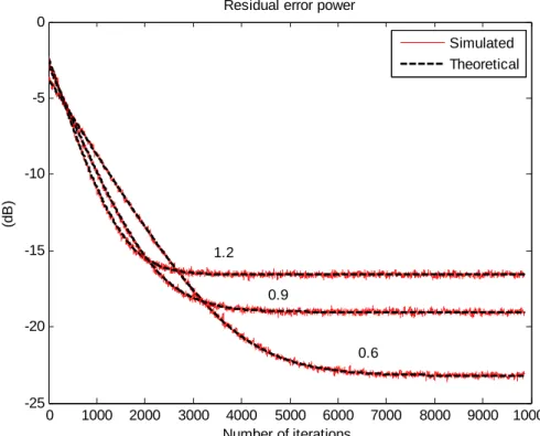
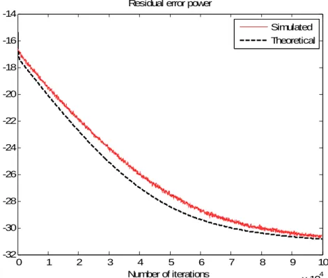
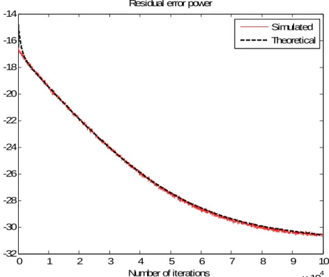
2 2 2 , 2 2 2 2 4 2 2 2 2 2 2 1 lim ( ) . 2 e e e s s s h v s o o h s s h x h s M M E n M σ σ μ σ σ μ σ σ μ σ →∞ + + − = − h h ε (3.2.17)

By examining the matrix A in Eq. (3.2.16), we can see that the convergence rate is a monotonic increasing function of the step-size μh and the variance

2

s

σ of PWL processor output. Moreover, in Eq. (3.2.17) the steady-state of the 2nd moment of

( ) h n

ε increases with an increase of the near-end noise variance 2

v

σ , the step-size

h

μ , the PWL output power 2

s

σ , and the nonlinearity factor 2 ,e s s σ and 2 e s σ . We will

simulate this property in Chapter 5.

iteratively. By plugging Eq. (3.2.7) into (3.2.13) and denoting

(

2 2 4

)

1 1 2 h s h s K = − μ σ +μ Mσ , ₂ 2

(

2 2 2 2

)

e e h s h s s K = −μ σ +μ Mσ σ and

(

2

)

2 2 2 2 2 3 h s v s se o ₂ K =μ Mσ σ +Mσ σ h , we have

{

2

}

{

2

}

{

}

1 2 3 2 2 ( ) ( 1) T ( 1) h h o h E ε n ≈K E ε n− +K h E ε n− ⋅ +K

{

}

{

}

{

}

2 1 2 2 3 2 2 2 , 3 ( 2) ( 2) (1- ) ( 2) e T h o h T o h s h h s s o K E n K E n K K μ σ E n μ σ K ⎡ ⎤ = _⎢ − + − + _⎥ ⎣ ⎦ ⎡ ⎤ + _⎣ − − _⎦+ ε h ε h ε h

{

}

{

}

{

}

2 1 1 1 ₂ 2 3 2 2 2 2 2 1 1 1 2 2 2 2 2 , 1 1 1 3 2 2 1 1 (0) ( 2) (1- ) (1- ) (1- ) (1- ) (0) 1 1 (1- ) (1- ) ( e n T h o h n T h s h s h s o n h s h h s s o h s h s K K E K E n K K K K K E K K K K K K μ σ μ σ μ σ μ σ μ σ μ σ μ σ − − − ⎡ ⎤ = _⎢⎣ + ⋅ − + _⎥⎦ ⎡ ⎡⎡ ⎤ ⎤ ⎤ +_{⎣ ⎣⎣} + _⎦ + _⎦ + _⎦ ⋅ ⎡ − ⎤ ⎡+ +_⎣ + + + ⎤_⎦ ⎣ ⎦ ⎡ ⎤ ⎡ ⎤ − +_⎣ + _⎦+ _⎣ + _⎦ ε h ε h ε h

{

}

2 2 1 2 2 2 2 2 3 2 1 1 1 , 2 2 1- ) (1- ) (1- ) (1- ) e h s n h s h s h s h s s o K K K K K μ σ μ σ μ σ μ σ − μ σ ⎡ ₊ ⎤_{+ +} ⎣ ⎦ ⎡ ⎡_⎣⎡_⎣ + ⎤_⎦ + ⎤_⎦ + ⎤ ⎣ ⎦ h

{

}

{

}

{

2 2 2 2 2 1 1 ₂ 1 1 1 2 2 2 2 2 , 3 1 1 1 2 2 2 2 1 1 1 2 (0) (1- ) (1- ) (1- ) (1- ) (0) 1 1 (1- ) (1- ) (1- ) (1-e n n h h s h s h s T n o h s h h s s o h s h s h s h s K E K K K K E K K K K K K K μ σ μ σ μ σ μ σ μ σ μ σ μ σ μ σ μ σ − − ⎡ ⎡⎡ ⎤ ⎤ ⎤ = +_{⎣ ⎣⎣} + _⎦ + _⎦ + _⎦ ⎡ ⎤ ⎡ ⎤ ⋅_⎣ − _⎦+ _⎣ + + + + _⎦ ⎡ ⎤ ⎡ ⎤ ⎡ ⎤ − +_⎣ + _⎦+_⎣⎣ + _⎦ + _⎦+ + ε h ε h

}

2 2 2 2 2 2 1 1 1 , 2 2 ) (1- ) (1- ) e n h s h s h s s o K μ σ K μ σ K − μ σ K ⎡ ⎡_⎣⎡_⎣ + ⎤_⎦ + ⎤_⎦ + ⎤ ⎣ ⎦ h

Using the geometric series formula, it can be simplified as:

{

2

}

{

2

}

2 ₁

{

}

2 2 ₁2 1 2 2 2 2 2 1 1 2 3 3 2 1 1 2 2 1 1 1 , 2 3 2 2 2 1 1 1 (1- ) (1- ) ( ) (0) (0) 1 (1- ) (1- ) (1- ) (1- ) 1 (1- ) (1- ) e 1 n n n h s T h s h h o h h s h s n n n h s h s h s s o h s h s K K E n K E K E K K K K K K K K K K μ σ μ σ μ σ μ σ μ σ μ σ _{μ σ} μ σ μ σ − − ⎡ − − ≈ + − +_⎢ − _⎣ − ⎤ − − − + + + _⎥ + − − _⎦ − ε ε h ε h

{

2

}

2 ₁

{

}

1 2 2 2 2 (1- ) 1 (0) (0) (1- ) (1- ) n n n h s T h o h K K E K E K K μ σ μ σ μ σ − = + − − − ε h ε

{

}

{

}

{

}

2 _{3 2} 2 , 2 2 2 2 2 1 1 1 2 2 , 2 2 2 2 2 2 2 1 1 2 ₂ 1 2 1 1 1 ( ) 1 (1 ) 1 (0) (1 ) (1 ) (1- ) (0) e e h h s s o h s h s T h s s o o h n h s h s h s h s n h K E n K K K K K K E K K K K E μ σ μ σ μ σ μ σ μ σ μ σ μ σ μ σ ⎡ ⎤ ≈ − _⎢ − _⎥ − − − _⎣ − _⎦ ⎡ ⎤ ⎢ ⎥ + − + + − − ⎡ − ⎤ ⎢ _{⎣ ⎦}⎥ ⎣ ⎦ + − ε h h h ε h ε

{

}

2 2 , 2 2 3 2 2 1 1 1 1 (0) (1 ) (1 ) (1- ) 1 e T h s s o o h h s h s K E K K K K K μ σ μ σ μ σ ⎡ ⎤ ⎢ − − ⎥ − − − ⎡ − ⎤ − ⎢ _{⎣ ⎦} ⎥ ⎣ ⎦ h ε (3.2.18) The expression of the 2nd moment of linear coefficient weight error in Eq. (3.2.18) appears to be tedious, as compared to the compact vector form in Eq. (3.2.16).

Let us consider the special case of perfect PWL coefficients. The second moment of εh i_,( )n can be easily obtained by setting the nonlinear coefficient weight error

0 = w ε so that A₂ =A₃ = i.e.,0 2 1 ₂ 2 h v h s M K M μ σ μ σ =

− and K2 = . The Eq. (3.2.18) 0

reduces to

{

2

}

₃

{

2

}

₃ 1 2 2 1 1 ( ) (0) 1 1 n h h K K E n K E K K ⎡ ⎤ ≈ + _⎢ − _⎥ − _⎣ − _⎦ ε ε

which is a well known result [3].

Finally, after derivation of first and second moments of the linear coefficient weight error, we turn our attention to the residual output power. From Eq. (3.2.2), the mean square error (i.e., residual error) is given by

{ }

2 ( ) ( ) h J n =E e n

{

}

{

}

{

}

{

}

2 E ( ) ( ) ( ) ( ) ( ) ( ) 2 E ( ) ( ) ( ) . T T T T v o e e o h h T T o e n n E n n n n n n E n σ = + ⋅ + ⋅ ⋅ ⋅ + ⋅ ⋅ ⋅ _h h s s h ε s s ε h s s ε (3.2.19)

Because the variation of εh( )n is slow compared to ( )s n , hence

{

}

₂

{

2

}

2 ( ) ( ) ( ) ( ) ( ) T T h h s h E ε n ⋅s n ⋅s n ⋅ε n =σ E ε n (3.2.20)

{

}

{

}

2 2 2 2 2 2 , 2 2 ( ) ( ) 2 ( ) . e e T h v s o s h s s o J n =σ +σ h +σ E ε n + σ h ⋅E ε_h n (3.2.21)

which depends on the E

{

ε_h( )n

}

and the .E

{

ε_h( )n 2₂

}

that are derived earlier in Eq.

(3.2.7) and (3.2.18) or the compact Eq. (3.2.16).

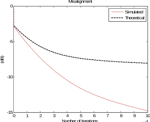
3.3 Convergence analysis of joint adaptation of linear and PWL

coefficients

After the convergence of linear coefficients, the nonlinear adaptive filter switches to the 2nd stage in which linear and PWL coefficients will be updated jointly. Now, the residual error is given by

( ) ( ) T T( ) ( ) T( ) T( ) T( ) T( ) ( )

o h w o w h

e n =v n −w F⋅ n ⋅ε n −ε n ⋅F n ⋅h −ε n F n ε n (3.3.1)

The coupled linear and nonlinear weight error in the fourth term of Eq. (3.3.1) renders difficulty in convergence analysis. However, with wide band signal like speech, loudspeaker nonlinearities are much less dominant than the linear components in general. Therefore, we can assume initial PWL weight error is much smaller than optimal PWL coefficients. Moreover, the converged linear coefficients would be approximately to optimal linear filter, namely,

( ) h n << o

ε h , εw( )n <<w , (3.3.2) _o

where ( )εw n =w( )n −w . With sufficiently small perturbation errors in linear and o nonlinear coefficients in Eq. (3.3.2), the 2nd-order perturbation term can be discarded and the estimation error becomes

( ) ( ) T T( ) ( ) T( ) T( )

o h w o