友矩陣和規範算子的數值域

國 立 交 通 大 學

應用數學系

碩士論文

Numerical Ranges of Companion Matrices

and Normal Operators

研究生 : 陳育慈

指導老師 : 吳培元 教授

友矩陣和規範算子的數值域

Numerical Ranges of Companion Matrices

and Normal Operators

研 究 生：陳育慈 Student：Yu-Tzu Chen

指導教授：吳培元 Advisor：Dr. Pei Yuan Wu

國 立 交 通 大 學

應 用 數 學 系

碩 士 論 文

A Thesis

Submitted to Department of Applied Mathematics

College of Science

National Chiao Tung University

In partial Fulfillment of the Requirements

For the Degree of Master

In

Applied Mathematics

June 2007

Hsinchu, Taiwan, Republic of China

友 矩 陣 和 規 範 算 子

的 數 值 域

研 究 生：陳育慈

指導老師：吳培元 教授

國 立 交 通 大 學

應 用 數 學 系

摘

要

在本篇論文中，我們研究兩類算子的數值域。針對友矩陣部分，我們

證明

可分解友矩陣的數值域會包含相對應的

友矩陣的數值域的

充要調件為

可分解友矩陣的行列式值的絕對值會大於 1。然而，相對

應的結果在一般的

可分友矩陣並不正確。針對規範算子的部份，我

們將數值域以乘積算子的表現函數來表示。

中 華 民 國 九 十 六 年 六 月

Numerical Ranges of Companion Matrices

and Normal Operators

Student: Yu-Tzu Chen

Advisor: Pei Yuan Wu

Department of Applied Mathematics National Chiao Tung University

Abstract

In this thesis, we study the numerical ranges of two kinds of operators. For companion matrices, we show that the numerical range of a 3-by-3 reducible companion matrix C(p) contains the numerical range of the 2-by-2 companion matrix C((1/3)p0_{) if and only if the absolute value of its determinant is greater}

than 1. However, the corresponding assertion for n-by-n reducible companion matrices is false. For a normal operator, we express its numerical range in terms of the function in its multiplication operator representation.

致 謝

我的論文得以完成，要感謝許多人在我碩士班期間給予

我的支持與幫忙，不論是學業上或是生活上。

首先要感謝的是我的指導老師吳培元教授，他是一個嚴

肅，有要求的人，在求學期間，我跟他學習到了非常多有用

的知識，並感謝老師不厭其煩的修正我的論文內容。另外，

要感謝的是博士班學長蔡明誠，經常與我討論論文的內容與

可能需要用到的背景知識。感謝跟我同研究室的劉筱凡，張

雁婷，容忍我寫論文遇到瓶頸的壞脾氣以及幫助我在論文內

文的修辭。感謝陳宜廷同學，常常講笑話調劑我的身心。

最後要感謝我的父母與家人，謝謝他們長久以來的支

持，讓我可以無後顧之憂的專心於完成論文。

Contents

Abstract (in Chinese) i

Abstract (in English) ii

Acknowledgement iii

1 Introduction 1

2 Companion Matrices 3

3 Normal Operators 15

1

Introduction

Let A be a bounded linear operator on the complex Hilbert space H. The numerical range of A is the set of complex numbers of the form hAx, xi, where x is any unit vector in H and h·, ·i denotes the inner product in H. We denote it by W (A). Namely,

W (A) = {hAx, xi : x ∈ H, kxk = 1}.

If H is an n-dimensional space, then A can be seen as an n × n complex matrix. The information about the numerical range of an n × n complex matrix has been quite well known. The shape of W (A) for a 2 × 2 matrix A is known to be a (possibly degenerate) elliptic disc. More generally, the numerical range of an n × n (n ≥ 3) matrix can be expressed in terms of an algebraic curve associated with the matrix [6]. Consider a 3 × 3 reducible companion matrix A associated with a monic polynomial

p and the companion matrix B associated with the monic polynomial (1/3)p0_{. In}

Section 2, we will discuss the relation between W (A) and W (B). We prove that W (A) contains W (B) if and only if |detA| ≥ 1. We will also show that the corresponding result does not hold for a 4 × 4 reducible companion matrix.

If A is a normal operator on the Hilbert space H, it is known that the numerical range of A can be expressed by its spectral measure [2]. If H is separable, then there exists a σ-finite measure space (X, Ω, µ) and a function f in L∞_{(µ) such that A is}

unitarily equivalent to the multiplication operator Mf. In Section 3, we will show

that W (A) can be described by the behavior of f .

We now introduce the notations to be used in the following sections. The boundary of a subset 4 in the plane is denoted by ∂4. The convex hull of a set 4, denoted by 4∧_{, is the smallest convex set including 4. The interior of 4 is denoted by Int}

4. The closure of 4 is denoted by 4. A∗ _{is the adjoint operator of A. Next, we list}

properties of the numerical range of an operator.

Proposition 1.1. Let A be an operator on H. Then the following hold:

W (A) is compact.

(2) W (A + aI) = W (A) + a for any complex number a. (3) W (bA) = bW (A) for any complex number b.

(4) W (A) is a convex subset of C.

(1), (2) and (3) are easily obtained from the definition. (4) appeared in [4, p. 315].

It follows from the definition of the numerical range that the diagonal entries aii

of a matrix A are all in W (A).

Theorem 1.2. Let A and B be operators (on possibly different spaces). (1) If A is unitarily equivalent to B, then W (A) = W (B).

(2) If B dilates to A, then W (B) is contained in W (A). (3) If A = A1

L

A2, then W (A) equals the convex hull of W (A1)

S

W (A2).

Recall that B is said to dilate to A if A is unitarily equivalent to an operator matrix of the form

  B ∗

∗ ∗



. Both (1) and (2) can be derived directly from the definition. The proof of (3) can be found in [4, p. 116].

In what follows, we explore the relations between the numerical range and the spectrum of an operator. The spectrum of an operator A, denoted by σ(A), is the set of scalars z for which A − zI is not invertible. The point spectrum σp(A) of A is

the set of eigenvalues of A.

Theorem 1.3. For an arbitrary operator A, we have (1) σp(A) ⊆ W (A), and

(2) σ(A) ⊆ W (A).

(1) can be proved from the definition, and (2) is justified in [4, Problem 214].

2

Companion Matrices

Recall that for every complex monic polynomial p(z) = zn_{+ a}

1zn−1+ ... + an of

degree n, there is associated an n × n matrix

(2.1) C(p) =            0 1 0 1 . .. ... 0 1

−an −an−1 . . . −a2 −a1

           ,

called the companion matrix of p. Note that the characteristic polynomial and min-imal polynomial of C(p) are both equal to p. We say that a matrix is reducible if it is unitarily equivalent to the direct sum of two other matrices. The numerical ranges of 2-by-2 and 3-by-3 matrices have been known before. Here we give a brief sketch. Proposition 2.1. Let A be a 2 × 2 matrix unitarily equivalent to

  a b

0 c  . (1) If b = 0, then W (A) is the line segment with endpoints a and c.

(2) If b 6= 0 and a = c, then W (A) is the circular disc centered at a with radius

|b|/2.

(3) If b 6= 0 and a 6= c, then W (A) is the elliptic disc with foci a and c and with

the length of minor axis |b|.

The proof of this proposition is provided in [5, pp. 20–23].

To describe the numerical ranges of 3 × 3 matrices, we need some extra notions. A point in homogeneous coordinates is an ordered triple

(x, y, z)

of complex numbers x, y and z which are not all zero. Two such points (x1, y1, z1)

a 6= 0. Then the complex projective plane is the set of all the equivalence classes

[x, y, z]. That is,

CP2 = {[x, y, z] : (x, y, z) ∈ C3 _{− {0}}.}

The point [x, y, z] in CP2 with z 6= 0 can be mapped to the point (x/z, y/z) in nonhomogeneous coordinates. On the other hand, the point (x, y) in nonhomogeneous coordinates becomes [x, y, 1] in CP2. The points [x, y, 0] in CP2 are points at infinity. If C is an algebraic curve in CP2 _{given by p(x, y, z) = 0, where p is a homogeneous}

polynomial in x, y and z, then its dual curve C∗ _{is given by}

{[u, v, w] ∈ CP2 _{: ux + vy + wz = 0 is a tangent line of C}.}

For an n × n matrix A, Re A = (A + A∗_{)/2 and Im A = (A − A}∗_{)/(2i) denote the real}

and imaginary parts of A, respectively. Define the degree-n homogeneous polynomial

pA in x, y and z by

(2.2) pA(x, y, z) = det(xReA + yImA + zIn).

Kippenhahn [6] proved that the numerical range of an n × n matrix A can be de-scribed in terms of pA as follows.

Theorem 2.2. The numerical range of A equals the convex hull of the real points of

the dual curve of pA(x, y, z) = 0.

Next we state the classification for the numerical ranges of 3 × 3 matrices, which is also given by Kippenhahn [6].

Proposition 2.3. If A is a 3 × 3 matrix and pA is defined as in (2,2), then W (A)

can be classified into four classes:

(1) If pA is the product of three linear factors:

pA(x, y, z) = 3 Y j=1 (z + ajx + bjy), 4

then A is normal and W (A) is the closed triangular region with vertices (aj, bj), j =

1, 2, 3 (it may degenerate to a line segment or a point ).

(2) If pA is the product of a linear and an irreducible quadratic factor:

pA(x, y, z) = (z + ax + by)q(x, y, z),

then W (A) is the convex hull of the point (a, b) and the ellipse given by the dual curve of q(x, y, z) = 0. Hence W (A) is an elliptic disc possibly with a cone added to it; in the latter case, A is reducible.

(3) If pA is irreducible and the dual curve of pA= 0 has degree four, then W (A)

has a line segment on the boundary.

(4) If pA is irreducible and the dual curve of pA= 0 has degree six, then W (A) is

an oval set.

We now start to consider our problem on the numerical ranges of companion ma-trices. The next two results are from [3].

Proposition 2.4. If A is a companion matrix, then λA is unitarily equivalent to a

companion matrix for any λ, |λ| = 1.

This proposition says that if A is of the form         0 1 . .. ... 0 1 an an−1 . . . a1         ,

then λA is unitarily equivalent to the companion matrix         0 1 . .. . .. 0 1 λn_a n λn−1an−1 . . . λa1         .

The detailed proof can be found in [3, Lemma 2.8].

Theorem 2.5. An n × n (n ≥ 2) companion matrix A is reducible if and only if its

eigenvalues are of the form:

aωnj1, . . . , aωnjp, ( 1 ¯a)ωn jp+1_{, . . . , (}1 ¯a)ωn jn_,

where a 6= 0, ωn = exp(2πi/n) denotes the nth primitive root of 1, 1 ≤ p < n,

and {j1, . . . , jp} and {jp+1, . . . , jn} form a partition of {0, 1, . . . , n − 1}. In this case,

A is unitarily equivalent to A1

L

A2 with σ(A1) = {aωnj1, . . . , aωnjp} and σ(A2) =

{(1/¯a)ωnjp+1, . . . , (1/¯a)ωnjn}.

This theorem is verified in [3, Theorem 1.1].

The next theorem is our main result in this section. It partially solves a question posed by J. Zem´anek.

Theorem 2.6. Let A be a 3 × 3 reducible companion matrix and p be its associated

polynomial. For the monic polynomial (1/3)p0_{, there is associated a 2 × 2 companion}

matrix B. Then their numerical ranges W (A) and W (B) have the following contain-ment relations:

(1) W (A)TW (B) 6= ∅.

(2) If |detA| < 1, then W (B) * W (A).

(3) If |detA| ≥ 1, then W (B) ⊆ W (A). Moreover, ∂W (A)T∂W (B) = ∅ if |detA| > 1, and ∂W (A) intersects ∂W (B) at exactly three points if |detA| = 1. Proof. Since A and B are companion matrices, 0 is in both W (A) and W (B). This

proves (1).

For (2) and (3), we may assume by Theorem 2.5 that the eigenvalues of A are

a,1 aω, 1 aω 2_, 6

where ω = exp(2πi/3) is the 3rd primitive root of 1. Let e−iθ _{be such that ae}−iθ ₌

t > 0. Since the characteristic polynomial of A is p(z) = (z − a)(z − 1 aω)(z − 1 aω 2₎ = z3_{− (a −} 1 a)z 2_{− (}a a − 1 a2)z − a a2 = z3_{− (t −} 1 t)e iθ_z2_{− (1 −} 1 t2)e 2iθ_{z −} 1 te 3iθ_,

the 3 × 3 reducible companion matrix A is of the form      0 1 0 0 0 1 1 te 3iθ _{(1 −} 1 t2)e 2iθ _{(t −} 1 t)e iθ     . A direct computation shows that

1 3p 0_{(z) = z}2₋ 2 3(t − 1 t)e iθ_{z −} 1 3(1 − 1 t2)e 2iθ_,

and thus B is of the form   ₁ 0 1 3(1 − 1 t2)e 2iθ 2 3(t − 1 t)e iθ   .

It follows from Proposition 2.4 that e−iθ_{A is unitarily equivalent to}

     0 1 0 0 0 1 1 t 1 − 1 t2 t − 1 t     . Similarly, e−iθ_{B is unitarily equivalent to}

  ₁ 0 1 3(1 − 1 t2) 2 3(t − 1 t)   .

Hence we can assume that a > 0. Under this assumption, det A = 1/a > 0. Obvi-ously,

detA > 1 ⇔ a < 1, detA = 1 ⇔ a = 1, detA < 1 ⇔ a > 1.

Using Theorem 2.5, we derive that the reducible companion matrix A is unitarily equivalent to A1 M A2 = h a i M    1 aω b 0 1 aω 2    , where the entry b satisfies

a2_{+ |}1 aω| 2_{+ |b|}2_{+ |}1 aω 2_|2 _{= 1 + 1 + (}1 a) 2_{+ (1 −} 1 a2) 2_{+ (a −}1 a) 2_,

and can be taken to be nonnegative. A simple computation yields

b = |1 − 1 a2|.

Clearly, if a = 1, then b = 0. In this case, A is normal and W (A) is the regular triangular region with vertices 1, ω and ω2_{. When a 6= 1, the numerical range of A}

1

is the singleton {a}, and the numerical range of A2 is the elliptic disc with foci ω/a

and ω2_{/a and with the length of minor axis |1 − 1/a}2_{| by Proposition 2.1. Therefore}

the boundary of W (A2) is given by the equation

(x + 1 2a) 2 1 4(1 − 1 a2) 2 + y2 1 4( a4_{+ a}2_{+ 1} a4 ) = 1,

which we call ΓA. Note that the center of ΓA, labeled cA, is at −1/(2a). It is easy

to see that when a = 1, B =   0 1

0 0 

 and W (B) is the circular disc centered at 0 with radius 1/2. In this case, W (A) contains W (B) and their boundaries intersect at exactly three points. If a 6= 1, by a brief computation, B is unitarily equivalent to

   a2_{− 1 +}√_a4_{+ a}2_{− 2} 3a c 0 a2− 1 − √ a4_{+ a}2_{− 2} 3a    ,

where the nonnegative c satisfies

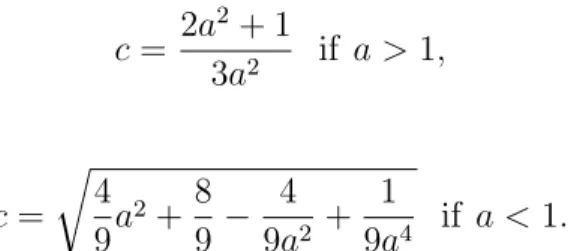
|a2− 1 + √ a4_{+ a}2_{− 2} 3a | 2_+|a2− 1 − √ a4_{+ a}2_{− 2} 3a | 2_+c2 _{= 1+(}1 3(1− 1 a2)) 2₊₍2 3(a− 1 a) 2_). 8

Hence the preceding equation yields c = 2a2+ 1 3a2 if a > 1, and c = r 4 9a2+ 8 9 − 4 9a2 + 1 9a4 if a < 1.

Again, Proposition 2.1 says that the numerical range of B is an elliptic disc and the boundary of W (B) is given by the equation

(x − a2− 1 3a ) 2 (2 9− 1 9a2 + 1 36a4 + a2 9 ) + y2 (2a 2_{+ 1} 6a2 ) 2 = 1,

which we call ΓB. Note that the center of ΓB, labeled cB, is at (a2−1)/(3a). Obviously,

the points a, cAand cB are on the x-axis and satisfy a > cB > cA. As the point a may

be in or out of (ΓA)∧, we have two different cases to consider. These are illustrated

in the following figures.

A

B

a _x

y

A B a

y

x

If a is in (ΓA)∧, then we need only check that ΓB is in the interior of (ΓA)∧.

This can be observed from Figure 1 visually. If a is not in (ΓA)∧, then let mA

(resp., mB) denote the slope of the tangent line from point a to ΓA (resp., ΓB). Since

W (B) ⊆ W (A) if and only if mA2 ≥ mB2, to complete the proof, we need compare the

magnitudes of mA2 and mB2. This can be observed from Figure 2. For convenience,

let b1and b2 denote one half of the lengths of the minor axis of ΓAand ΓB, respectively.

Our discussion is now divided into two cases: (a) If a is in (ΓA)∧, then d(a, cA) ≤ b1, that is,

|a − −1 2a| ≤ 1 2|1 − 1 a2|.

By computation, this holds if and only if a ≤ 1/2. We claim that in this case (2.3) b1 > d(cA, cB) + b2, that means (2.4) 1 2( 1 a2 − 1) > a 3 + 1 6a + r 2 9 − 1 9a2 + 1 36a4 + a2 9, and the point at the major axis of ΓB

(2.5) (a2− 1 3a , 2a2_{+ 1} 6a2 ) is in (ΓA) ∧_, 10

that means (2.6) ( a2_{− 1} 3a + 1 2a) 2 1 4(1 − 1 a2) 2 + (2a 2_{+ 1} 6a2 ) 2 1 4( a4_{+ a}2_{+ 1} a4 ) 6 1.

For a ≤ 1/2, (2,4) and (2.6) are easily seen to be true. From (2.3) and (2.5), it implies that ΓB is contained in the interior of (ΓA)∧, and hence W (B) ⊆ W (A).

(b) Assume that a is not in (ΓA)∧. The tangent lines from a to ∂ΓA are given by

y − 0 = mA(x − (− 1 2a)) ± r mA2(1 4(1 − 1 a2)2) + ( a4_{+ a}2_{+ 1} 4a4 ).

Since they pass through the point (a, 0), a calculation shows that

mA2 =

a4_{+ a}2_{+ 1}

4a6_{+ 3a}4_{+ 3a}2_{− 1}.

Applying this formula to B, one can get

mB2 = 4a4_{+ 4a}2_{+ 1} 12a6_{+ 8a}4_{+ 8a}2_{− 1}. Thereby it leads to mA2 mB2 = (a4+ a2+ 1)(12a6+ 8a4+ 8a2− 1) (4a4_{+ 4a}2_{+ 1)(4a}6_{+ 3a}4_{+ 3a}2_{− 1)}. Noting that

(a4_{+ a}2_{+ 1)(12a}6_{+ 8a}4_{+ 8a}2_{− 1) − (4a}4_{+ 4a}2_{+ 1)(4a}6_{+ 3a}4_{+ 3a}2_{− 1)}

= 4a2_(−a6_{+ 1)(a}2_{+ 2)}

is positive when 0 < a < 1 and negative when a > 1, we have mA2 < mB2 when a > 1

and mA2 > mB2 when a < 1. Notice that mA2 > mB2 means that the boundary of

W (A) intersects W (B) at no point.

As a conclusion, we have W (B) ⊆ W (A) when a < 1 and W (B) * W (A) when

For n × n (n ≥ 4) reducible companion matrices, assertion (2) in Theorem 2.6 is in general false.

Example 2.7. Let p(z) = (z−20)(z+1/20)(z−i/20)(z+i/20) be a monic polynomial. Then A =        0 1 0 0 0 0 1 0 0 0 0 1 1/400 399/8000 399/400 399/20       

is the associated 4 × 4 reducible companion matrix. The 3 × 3 companion matrix B associated with the monic polynomial (1/4)p0 _is

B =     0 1 0 0 0 1 399/32000 399/800 1197/80     .

Although det A = 1/400 < 1, the numerical range of B is contained in the numerical range of A. We prove this via Theorem 2.2. First, we calculate the homogeneous polynomial pA as follows. pA(x, y, z) = det        x        0 1/2 0 1/800 1/2 0 1/2 399/16000 0 1/2 0 799/800 1/800 399/16000 799/800 399/20        +y        0 −i/2 0 i/800 i/2 0 −i/2 399i/16000

0 i/2 0 −i/800 −i/800 −399i/16000 i/800 0

       + z        1 0 0 0 0 1 0 0 0 0 1 0 0 0 0 1               = det        z (x − iy)/2 0 (x + iy)/800

(x + iy)/2 z (x − iy)/2 399(x + iy)/16000

0 (x + iy)/2 z (799x − iy)/800

(x − iy)/800 399(x − iy)/16000 (799x + iy)/800 z + 399x/20

       12

= z4₊399 20xz 3_{− (}383520001 256 × 106 x 2₊128160001 256 × 106 y 2_)z2 −( 159201 16 × 103x 3₊ 159999 16 × 103xy 2_{)z +} 159201 64 × 104x 4₊ 160801 64 × 104x 2_y2 = (z+20x)(z3₋ 1 20z 2_x−128160001 256 × 106 z 2_y−127520001 256 × 106 zx 2₊ 160801 128 × 105y 2_x+ 159201 128 × 105x 3_). Similarly, pB(x, y, z) = z3₊1197 80 xz 2₋₍1281440801 4096 × 106 y 2₊3324320801 4096 × 106 x 2_{)z −}383838399 1024 × 105y 2_x−382561599 1024 × 105x 3_.

Hence W (A) is the convex hull of the point (20, 0) plus the dual curve of the polyno-mial z3₋ 1 20z 2_{x −} 128160001 256 × 106 z 2_{y −} 127520001 256 × 106 zx 2₊ 160801 128 × 105y 2_{x +} 159201 128 × 105x 3_.

W (B) is the convex hull of the dual curve of the polynomial z3₊1197 80 xz 2₋₍1281440801 4096 × 106 y 2₊3324320801 4096 × 106 x 2_{)z −}383838399 1024 × 105y 2_x−382561599 1024 × 105x 3_.

−2 0 2 4 6 8 10 12 14 16 18 20 −1 −0.8 −0.6 −0.4 −0.2 0 0.2 0.4 0.6 0.8 1 W(A) W(B) Figure 3: W (B) ⊆ W (A).

We believe that Theorem 2.6(3) should be true for n × n reducible companion matrices A, but its proof is too complicated to be written down explicitly here.

3

Normal Operators

Let A be a bounded linear operator on the complex Hilbert space H. The numerical range of an operator A is closely related to its spectrum. In fact, we have

W (A) ⊇ σ(A)∧_{. Recall that A is normal if AA}∗ _{= A}∗_{A. For such an A, W (A) and}

σ(A)∧ _{are even equal.}

Theorem 3.1. If A is a normal operator, then W (A) = σ(A)∧_.

Its proof can be found in [4, pp. 115–116].

Instead of its closure, the numerical range of a normal A can be expressed more precisely in terms of its spectral measure. We introduce the spectral measure and its properties first. Let X be a set, Ω be a σ-algebra of subsets of X, and H be a Hilbert space. B(H) denotes the algebra of bounded operators on H.

Definition 3.2. A spectral measure for (X, Ω, H) is a function

E : Ω → B(H) such that

(1) E(4) is an (orthogonal) projection for 4 ∈ Ω; (2) E(∅) = 0 and E(X) = I;

(3) E(41∩ 42) = E(41)E(42) for all 41 and 42 in Ω;

(4) if {4n} is a sequence of disjoint sets in Ω, then

E Ã [ n 4n ! =X n E(4n),

where P_nE(4n) denotes the convergence in strong operator topology.

Theorem 3.3. If A is normal on H, then there exists a unique spectral measure

such that

(1) EA(σ(A)) = I;

(2) A =R_σ(A)zdEA(z).

This theorem is verified in [1, pp. 263–264]. This unique measure EA is called the

spectral measure for A.

Next we describe W (A) in terms of its spectral measure.

Theorem 3.4. If A is normal, then the numerical range of A equals the interior of

σ(A)∧ _{plus the points z on the boundary ∂σ(A)}∧ _{for which the longest interval [z}

1, z2]

in ∂σ(A)∧ _{containing z is such that both E}

A([z1, z]) and EA([z, z2]) are nonzero.

Namely, W (A) = (Int σ(A)∧₎S_{{z ∈ ∂(σ(A)}∧_{) : [z}

1, z2] is the longest interval in

∂(σ(A)∧_{) containing z such that E}

A([z1, z]) 6= 0 and EA([z, z2]) 6= 0}.

Corollary 3.5. If A is normal, then the numerical range of A equals the intersection

of all convex Borel subsets 4 of C with EA(4) = I. Namely,

W (A) =\{4 ⊆ C : 4 Borel convex, EA(4) = I}.

Both this theorem and its corollary appeared in [2].

There is another representation for normal operators on a separable Hilbert space. In the following, we will express the numerical range of such a normal operator in terms of the ingredients in its representation. Let Ω be a σ-algebra of subsets of X and µ be a positive measure on Ω. For any f in L∞_{(µ), M}

f denotes the multiplication

operator Mfg = f g for g in L2(µ).

Theorem 3.6. If A is normal on a separable Hilbert space, then there exists a σ-finite

measure space (X, Ω, µ) and a function f in L∞_{(µ) such that A is unitarily equivalent}

to Mf on L2(µ). In this situation, σ(A) = σ(Mf) = essential range of f .

Recall that the essential range of f is defined as

ess. ran. (f ) =\{f (4) : 4 ∈ Ω and µ(X \ 4) = 0}.

The proof of this theorem is provided in [1, p. 265, and pp. 272–273].

The next two results are the expressions of the numerical range of a normal A in terms of the function f in the above representation.

Theorem 3.7. If A is normal on a separable Hilbert space and f is the function as

in Theorem 3.6, then the numerical range of A equals the interior of σ(A)∧ _{plus the}

points z on the boundary ∂(σ(A)∧_{) for which the longest interval [z}

1, z2] in ∂σ(A)∧

containing z is such that both µ(f−1_([z

1, z])) and µ(f−1([z, z2])) are positive. Namely,

W (A) = (Int σ(A)∧₎S_{{z ∈ ∂(σ(A)}∧_{) : [z}

1, z2] is the longest interval in ∂σ(A)∧

containing z such that µ(f−1_([z

1, z])) > 0 and µ(f−1([z, z2])) > 0}.

The following lemma is useful in proving the theorem.

Lemma 3.8. Let 4 be a convex subset of C and ν be a probability measure on 4.

Then we have _Z

4

zdν(z) ∈ 4.

The lemma is trivially the consequence of the theorem in [7].

Proof of Theorem 3.7. According to Theorem 3.6, we may assume that A = Mf on

L2_{(µ). If z is a point in the interior of W (A), then, by Theorem 3.1, z is in the}

interior of σ(A)∧_.

Let z be a point on ∂σ(A)∧ _{for which the longest interval [z}

1, z2] containing z is

such that µ(f−1_([z

1, z])) = 0. Assume that z is in W (A), that is, z = hAg, gi for some

z = hMfg, gi = Z X f |g|2_dµ = Z X\f−1_([z1,z]) f |g|2_dµ = Z f−1_(σ(A)∧_\[z1,z]) f |g|2dµ.

Define the measure ν by

ν(4) =

Z

4

|g|2_{dµ for 4 in Ω.}

Then ν is a probability measure and

z =

Z

σ(A)∧_\[z1,z]

wdν

by the Randon-Nikodym theorem. Since σ(A)∧_{\ [z}

1, z] is convex, Lemma 3.8 implies

that z is in σ(A)∧ _{\ [z}

1, z], a contradiction. Therefore, µ(f−1([z1, z])) > 0. Similarly,

µ(f−1_{([z, z}

2])) > 0. This proves one direction of the containment.

For the converse, if z is in the interior of σ(A)∧_{, then trivially z is in W (A). Let z}

be in ∂σ(A)∧ _{satisfying the asserted condition. Let g be a unit vector in L}2_{(µ) with}

g = 0 on X \ f−1_([z 1, z]). Then hAg, gi = Z X f |g|2_dµ = Z f−1_([z1,z]) f |g|2dµ,

which belongs to [z1, z] by Lemma 3.8. This shows that [z1, z]

T

W (A) is nonempty.

In the same way, we also have [z, z2]

T

W (A) is nonempty. Thus z is in W (A) by the

convexity of W (A).

Corollary 3.9. If A is normal on a separable Hilbert space and f is the function as

in Theorem 3.6, then the numerical range of A equals the intersection of all convex Borel subsets 4 of C with µ(X \ f−1_{(4)) = 0. Namely,}

W (A) = \{4 ⊆ C : 4 Borel convex, µ(X \ f−1_{(4)) = 0}.}

Proof. Let 4 be a convex Borel subset of C with µ(X \ f−1_{(4)) = 0. For any unit}

vector g in L2_{(µ), we have} z = hAg, gi = Z X f |g|2dµ = Z f−1₍₄₎ f |g|2_dµ,

which is in 4 by Lemma 3.8. Therefore we conclude that W (A) ⊆ 4. This implies that

W (A) ⊆\{4 ⊆ C : 4 Borel convex, µ(X \ f−1_{(4)) = 0}.}

Conversely, let B ≡T{4 ⊆ C : 4 Borel convex, µ(X \ f−1_{(4)) = 0}. We claim}

that B is contained in (Int σ(A)∧₎S_{{z ∈ ∂(σ(A)}∧_{) : [z}

1, z2] is the longest interval in

∂σ(A)∧ _{containing z such that µ(f}−1_([z

1, z])) > 0 and µ(f−1([z, z2])) > 0}. If z is

in the interior of B, then z is in the interior of σ(A)∧_{. For the other case, z is in B}

and also on the boundary ∂B of B. Let [z1, z2] be the longest interval in ∂(σ(A)∧)

containing z. If µ(f−1_([z

1, z])) = 0, then 4 ≡ σ(A)∧\ [z1, z] is Borel convex and

µ(X \ f−1(4)) = µ(X \ (f−1(σ(A)∧) \ f−1([z1, z]))) = 0.

Then B ⊆ 4 and hence z is in 4, a contradiction. Therefore, we must have

µ(f−1_([z

1, z])) > 0. Similarly, µ(f−1([z, z2])) > 0. We conclude from Theorem 3.7

References

[1] J. B. Conway, A Course in Functional Analysis, 2nd ed., Springer, New York, 1990.

[2] E. Durszt, On the numerical range of normal operators, Acta Sci. Math. (Szeged) 25 (1964), 262–265.

[3] H.-L. Gau, P. Y. Wu, Companion matrices: reducibility, numerical ranges and similarity to contractions, Linear Algebra Appl. 383 (2004), 127–142.

[4] P. R. Halmos, A Hilbert Space Problem Book, 2nd ed., Spinger, New York, 1982. [5] R. A. Horn, C. R. Johnson, Topics in Matrix Analysis, Cambridge University

Press, Cambridge, 1991.

[6] R. Kippenhahn, ¨Uber den Wertevorrat einer Matrix, Math. Nachr. 6 (1951), 193–228.

[7] H. Rubin, O. Wesler, A Note on convexity in Euclidean n-space, Proc. Amer.

Math. Soc. 9 (1958), 522–523.