在無線區域網路下省電排程方法的研究

全文

(1)國立交通大㈻ ၥଉऋᏰ‫ف‬ġ 碩士論文. 在無線區域網路下省電排程方法的研究 A Power-Saving Scheduling for IEEE 802.11 Wireless Local Area Networks. 研究生：林曉伯指導教授：簡榮宏. 教授. 中華民國九十四年六月.

(2) 在無線區域網路下省電排程方法的研究. 研究生：林曉伯. 指導教授：簡榮宏博士. 國立交通大學資訊科學研究所. 摘. 要. 對無線區域網路之行動裝置而言，節約電源是決定系統運作壽命的關鍵因素，本篇論文提出一個具負載知覺之省電排程法，藉由有效的安排節點之甦醒時機，使得一個無線存取點下所服務的節點，在同一時槽(time slot)醒來的節點個數為最小，以減少競爭的節點數量。除此之外，我們提出避免競爭之流量排程法，讓節點依照不同的屬性來安排其存取順序，這些方法分別為單一節點存取、最小聯結代碼(AID)優先與最小暫存資料優先等。模擬結果顯示，具負載知覺之省電排程法與避免競爭之流量排程法兩者在電力節約上可以比原先無線區域網路標準定義的省電模式效果更好，同時也達到減少碰撞的目的。. i.

(3) A Power-Saving Scheduling for IEEE 802.11 Wireless Local Area Networks Student：Hsiao-Po Lin. Advisor：Dr. Rong-Hong Jan. DEPARTMENT OF COMPUTER AND INFORMATION SCIENCE NATIONAL CHIAO TUNG UNIVERSITY. Abstract Power saving is a significant problem for a battery-powered device, especially when it has an IEEE 802.11 wireless LAN communication module. In this thesis, we proposed a novel traffic scheduling algorithm for 802.11 WLANs, named Load-Aware Wakeup Scheduling (LAWS). LAWS lowers the amount of stations which contend for transmitting data by efficiently scheduling their wakeup time. This thesis also proposes another traffic scheduling mechanism, named Contention Avoidance Traffic Scheduling (CATS). The access sequence of mobile stations in CATS is scheduled via different parameters. They are classified into Multiple Wakeups Single Access (MWSA) and Smallest AID First (SAF) Smallest Queue Length First (SQLF). Simulation results showed that both LAWS and CATS outperform the original IEEE 802.11 standard in saving energy and have less packet collision.. ii.

(4) Contents 1 Introduction. 4. 2 Related Works. 10. 2.1. IEEE 802.11 Power Saving Mode . . . . . . . . . . . . . . . . . . .. 10. 2.2. Traffic Scheduling . . . . . . . . . . . . . . . . . . . . . . . . . . . .. 12. 3 Load-Aware Wakeup Scheduling. 16. 4 Contention Avoidance Traffic Scheduling. 23. 4.1. Multiple Wakeups Single Access . . . . . . . . . . . . . . . . . . . .. 23. 4.2. Multiple Wakeups Multiple Accesses . . . . . . . . . . . . . . . . .. 26. 4.2.1. The Smallest AID First . . . . . . . . . . . . . . . . . . . .. 27. 4.2.2. The Smallest Queue Length First . . . . . . . . . . . . . . .. 29. 5 Simulation and Results. 31. 5.1. Performance Metrics and Environment Setup . . . . . . . . . . . . .. 31. 5.2. Results and Discussion . . . . . . . . . . . . . . . . . . . . . . . . .. 33. 6 Conclusion and Future Work. 37. 1.

(5) List of Tables 3.1. A seuqence of wi (t) and n(t). . . . . . . . . . . . . . . . . . . . . .. 3.2. A sequence of wi (t) and n(t) after station J joins in power saving mode. . . . . . . . . . . . . . . . . . . . . . . . . . . . . . . . . . .. 3.3. 17. 18. A sequence of wi (t) and n(t) after station J with first wakeup time t5 . . . . . . . . . . . . . . . . . . . . . . . . . . . . . . . . . . . . .. 18. 3.4. The wakeup stations of beacon interval t3 to t8 . . . . . . . . . . . .. 20. 3.5. The wakeup stations of beacon interval t3 to t8 with station J scheduled in t3 . . . . . . . . . . . . . . . . . . . . . . . . . . . . . . . . .. 3.6. The wakeup stations of beacon interval t3 to t8 with station J scheduled in t4 . . . . . . . . . . . . . . . . . . . . . . . . . . . . . . . . .. 3.7. 20. 21. The wakeup stations of beacon interval t3 to t8 with station J scheduled in t5 . . . . . . . . . . . . . . . . . . . . . . . . . . . . . . . . .. 21. 3.8. To show the current status of the AP in wakeup counter form.. . .. 22. 5.1. Detail simulation configurations.. . . . . . . . . . . . . . . . . . . .. 32. 2.

(6) List of Figures 1.1. Adaptive power control algorithm.. . . . . . . . . . . . . . . . . . .. 6. 1.2. Level two header aggregation. . . . . . . . . . . . . . . . . . . . . .. 7. 1.3. On-demand paging scheme. . . . . . . . . . . . . . . . . . . . . . .. 9. 2.1. IEEE 802.11 power saving mode. . . . . . . . . . . . . . . . . . . .. 12. 2.2. Power management in IBSS in IEEE 802.11.. . . . . . . . . . . . .. 14. 4.1. Multiple Wakeup Single Access.. . . . . . . . . . . . . . . . . . . .. 25. 4.2. Multiple Wakeup Single Access without age. . . . . . . . . . . . . .. 26. 4.3. Multiple Wakeup Single Access with age.. . . . . . . . . . . . . . .. 27. 4.4. An example of the smallest AID first method. . . . . . . . . . . . .. 29. 4.5. An exmaple of the smallest queue length first method. . . . . . . .. 30. 5.1. The average sleeping time.. 33. 5.2. The throughput of each scheme.. 5.3. The latency of a successful transmission for each scheme.. 5.4. The improving rate of sleeping time (compared with PS mode of IEEE 802.11).. . . . . . . . . . . . . . . . . . . . . . . . . . . . . . . . . . . . . . . . . . . . . . .. . . . . . . . . . . . . . . . . . . . . . . . . . . . . .. 3. 34 35. 36.

(7) Chapter 1 Introduction Recently, the portable devices (or mobile devices) become more and more popular. In order to access the internet, supporting wireless communication becomes a primary function of those portable-devices. There are many wireless communication techniques, such as IEEE 802.11 [1, 2, 3], Bluetooth [4], GSM/GPRS, WCDMA [5], and etc. Among all of those wireless communication techniques, IEEE 802.11 is the one that most venders supported in their products. A common characteristic of these portable devices is the energy sources coming from their equipped battery. Once the battery energy drains out, these portable devices are out of function. Thus, power saving is a very important issue for prolonging the operation of a portable device. A survey [6] presents a comprehensive summary of work addressing energy efficient and low-power design within all layers of the wireless network protocol stack.. Many kinds of power-saving mechanisms have been proposed for portable devices [7, 8]. For example, while system in idle state, mobile devices can shut down the display components or decrease its brightness, replace the normal system clock with a low frequency one, and turn off the communication components 4.

(8) temporarily [7]. A statistic report [9, 10] have shown that the most portion of power in a portable device is consumed by its display and communication components. So, the effort of power saving must be made on display or communication component. This can lead to great power savings in the portable device. We focuses on power conservation in communication components.. Considering the power saving of mobile stations, the IEEE 802.11 standard specifies two states for them, they are Awake state and Doze state. While a station is in Awake state, its power is fully supplied and it is ready for transmitting or receiving data. In Doze state, a station uses a low power circuit to maintain the basic clock operation. Transmitting and receiving are not available under this clock. Feeney [9] has shown that switching to Doze state smartly will make significant energy saving for mobile stations.. For an IEEE 802.11 embedded mobile device, many methodologies have been proposed to save the power consumed by communication components. A common used method [11, 12] is controlling the listen interval of the wireless communication components. Listen interval is that each station will wakeup to listen beacon frame after a constant multiple of beacon duration. A dynamic listen-interval adaptation mechanism is proposed in [11]. Mobile station will dynamically adapt the duration of listen-interval according to the traffic situation. Thus, if a mobile device is not willing to transfer data, it can set a longer listen-interval for staying in sleep or low power mode. Mechanism proposed in [12] is similar to the one proposed in [11] but using both linear and exponential increasing to control the size of listeninterval. According to the analyzing results, sleeping duration is tradeoff with 5.

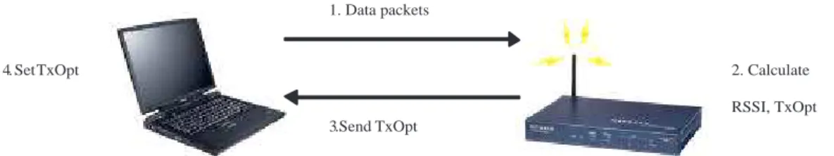
(9) communication delay. Another kind of listen interval controlling is the quorum based scheme [13, 14]. In the quorum based scheme, each station in power-saving mode synchronizes its wakeup schedule with each other such that the station can deliver buffered frames to a power-saving station at right time when the radio of power-saving station is turn on.. Controlling the transmission power can also saving the power of portable devices [12]. The basic idea is using the minimum power for sending data to the destination. A power control algorithm that adaptively adjusts the transmit power of transceiver is proposed in [12] to save power. Here we give a little example, shown in figure 1.1, to present the mechanism. At first, the mobile station sends data packets to base station. The base station calculates the optimal transmission power according to its received signal strength of the packet sent by mobile station. After that, base station sends the packet containing the optimal transmission power parameter back to the mobile station. Mobile station adjusts its transmission power to the one in the returned packet.. 1. Data packets. 4. SetTxOpt. 2. Calculate RSSI, TxOpt 3.Send TxOpt. Figure 1.1: Adaptive power control algorithm. Frame aggregation which fuses or integrates data to a small one is another way for saving energy [15]. For example, multiple consecutive frames can be con6.

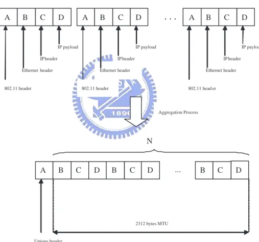
(10) densed into a single one so that the overhead of frame header can be reduced. In infrastructure mode, each header of frames for the AP to the same destination mobile station is the same. Thus, if multiple small frames can be fused as a big one, we can reduce the overhead of header during transmitting data. For example, as the figure 1.2 shows, N small frame are condensed into a big one by remove the redundant layer 2 headers. The more frames we condensed, the higher throughput we will gain.. A. B. C. D. A. B. C. D. IP payload. .... A. B. C. IP payload. IP header. IP payload. IP header. Ethernet header. IP header. Ethernet header. 802.11 header. D. Ethernet header. 802.11 header. 802.11 head er. Aggregation Process. N. A. B. C. D. B. C. D. .... B. C. D. 2312 bytes MTU. Unique header. Figure 1.2: Level two header aggregation. Another interesting way to saving power is using a low power radio module,. 7.

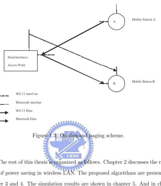
(11) such as bluetooth [16], or a special signaling channel [17]. As the on-demand paging system, a low power radio module, such as Bluetooth, is used to actuate the higher power radio circuit. So the battery can endure longer usage than the one without this mechanism. For example, mobile station A wants to communicate with mobile station B, where both A,B associate with the same AP as shown in figure 1.3. At first, mobile station A opens its 802.11 interface for transmitting data to AP. And AP uses its Bluetooth interface to wake up 802.11 interface of mobile station B. Secondly, the AP sends data to mobile station B by using its 802.11 interface. When the data exchange finishes, the AP uses the Bluetooth interface to send a message to mobile station B to command mobile station B power down its 802.11 interface. Therefore, the energy is saved by turning off the higher power consumption communication component - IEEE 802.11 interface. PAMAS is a similar approach that it uses a separate signaling channel [17]. The unique feature of this protocol is that it conserves battery power at nodes by intelligently powering off nodes that are not actively transmitting or receiving packets.. In this thesis, we proposed a novel algorithm for IEEE 802.11 infrastructure mode, named Load-Aware Wakeup Scheduling (LAWS). LAWS minimizes the contention of those PS mode mobile stations by efficient scheduling the wakeup time of a new coming station. In order to reduce the contention between the stations, this paper also proposed another algorithm, named Contention Avoidance Traffic Scheduling (CATS). Both LAWS and CATS just do a minor modification to the original IEEE 802.11 but introduces transparently benefits on energy saving. The simulation results showed that the proposed algorithms are better than the PSM of IEEE 802.11. 8.

(12) A. Mobile Station A. Dual interfaces Access Point. B. Mobile Station B. 802.11 interf ace Bluetooth interface 802.11 Data Bluetooth Data. Figure 1.3: On-demand paging scheme.. The rest of this thesis is organized as follows. Chapter 2 discusses the related works of power saving in wireless LAN. The proposed algorithms are presented in Chapter 3 and 4. The simulation results are shown in chapter 5. And in chapter 6, we give the conclusion and the future work.. 9.

(13) Chapter 2 Related Works This chapter discusses the previous works of IEEE 802.11 power saving mechanism in wireless LAN network. At first, we review the power saving mechanism defined in IEEE 802.11 standard. Secondly, we give a similar power saving mechanism that is applied for ”ad hoc mode” [18]. This mechanism is designed for IEEE 802.11 ad hoc mode. For applying to infrastructure mode, this mechanism must be modified or a new approach should be developed.. 2.1. IEEE 802.11 Power Saving Mode Mobile stations need power saving because their energy is constrained.. Therefore, in the power saving mechanism of IEEE 802.11 standard [1], mobile station sets power management bit of Frame Control Field to 1 for indicating whether it should enter sleeping mode. When the AP receives frames, it can be informed which station will enter sleeping mode. After then, stations will sleep until next beacon frame arrival and wake up to listen coming beacon frame. The AP knows which station enter sleeping mode, so it can monitor the traffic to station and buffer data for the station. Thus, stations can sleep without dropping 10.

(14) any frame. Finally, active and sleep switching is allowed if station have finishing its frames exchange or the AP have no data for it.. Mobile stations in sleeping mode will wake up periodically for listening to the beacon frame signal. Mobile station was assigned an Association ID code (AID) when it associated with AP. The traffic indication map (TIM) shall identify the mobile stations whether traffic is buffered in AP or not. Then the AP transmits a TIM with every beacon. Mobile station should wake up and enter Awake state for listening the beacon signal. If the corresponding bit of the mobile station is set to 1, it should remain in Awake state within whole the beacon interval and waiting for receiving buffered data. In figure 2.1 we can see the simple example representing the IEEE 802.11 power saving mode procedure. Mobile stations send PS-Poll frame to AP for getting the buffered data. If more than one station have data buffered in the AP, these station should use random backoff algorithm to determine access sequence. Each PS-Poll frame can be only used to retrieve one buffered frame. If mobile station has more than one frame buffered by the AP, the More Data bit in Field Control will set to 1 to indicate the station keeps on awaking for receiving buffered data.. There is a field which named Listen Interval while station executing the association request. It means how many beacon intervals the mobile station should wake up. Thus, the longer the station’s listen interval, the more buffer space AP should be reserve for the station. The AP has the charge to buffer data for sleeping stations. It should wait for at least one listen interval time before dropping the buffered frames of station. 11.

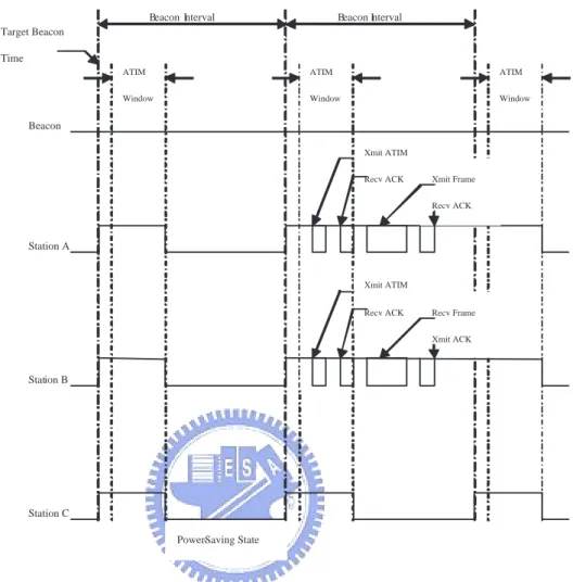
(15) Beacon interval. TIM (in Beacon). Data. TIM (in Beacon). TIM (in Beacon). AP. STA PS-Poll. ACK. Figure 2.1: IEEE 802.11 power saving mode.. Because station must contend the medium to get the chance for transferring data in the original IEEE 802.11 power saving mode, it will cause extra overhead in waiting for random backoff time slots. Besides, stations may wake up for a whole beacon interval but cannot get the chance to transfer data. The reason is that there are too many stations wake up at the same beacon interval to saturate the upper limit of traffic capacity. Therefore, we improve the original IEEE 802.11 power saving mode to let stations transferring data more efficient and avoid this condition. We will explain the proposed algorithm in next chapter.. 2.2. Traffic Scheduling Figure 2.2 is a power saving operation instance in IEEE 802.11 ad hoc. mode. Because these power saving mobile stations in ad hoc mode must contend the medium for the chance to transfer data, they will pay extra overhead in waiting a random backoff time. In addition, a station may wake up during whole beacon interval but cannot transfer it data out, this results from too many stations wake 12.

(16) up within the same beacon interval and all transferring data of wake up stations can’t be scheduled into single beacon interval. Thus, an enhanced power-saving algorithm [18] that uses a contention-free scheduling function to transfer data is proposed to solve this problem.. At first, this algorithm schedules the data transfer precedence of each station. To decide the precedence, each station exchanges scheduling information with others. So that each station can know what time its data should be transferred. After that, all stations can transfer data based on the precedence. Besides, this paper also proposes an idea to adjust the length of beacon interval so that all stations can transfer their data within this beacon interval. The length of the beacon interval will be calculated according to the total amount of transferring data.. All stations in ad hoc mode contend ATIM window of each beacon interval. After then stations that successfully send within ATIM windows are sorted based on the number of packets. Finally, the lengths of packets are cumulated and then the size of beacon interval which is long enough of all desired transferring data is decided. There is a little tricky that we let stations with fewer packets to transfer process earlier than those with more packets. This makes more station enter the Doze state early within the beacon interval.. This paper only describes the way to tuning beacon interval for tuning beacon interval to let all stations can transmit in this beacon, which is achieving power saving. This schedule method has to modify the access mechanism of the IEEE 802.11 standard. Besides, extra long beacon intervals may cause intolerable delay 13.

(17) Beacon Interval. Beacon Interval. Target Beacon Time ATIM. ATIM. ATIM. Window. Window. Window. Beacon Xmit ATIM Recv ACK. Xmit Frame Recv ACK. Station A. Xmit ATIM Recv ACK. Recv Frame Xmit ACK. Station B. Station C Power-Saving State. Figure 2.2: Power management in IBSS in IEEE 802.11. to the stations which have higher QoS requirement. Thus, it is not well enough for applying to infrastructure mode directly.. For efficiently supporting the infrastructure mode operation, we propose a novel traffic scheduling algorithm which use determining stations wake up time and choose which station have the access to the medium to satisfy the requirement of power saving over infrastructure mode. In the next chapter we will explain detailed algorithm about the traffic scheduling method in infrastructure mode. And. 14.

(18) also concerns about the different attributes in infrastructure mode, such as listen interval.. 15.

(19) Chapter 3 Load-Aware Wakeup Scheduling Note that if many stations have buffered frames in AP and their wakeup time is at the same beacon interval, these stations will ramp up and use the random backoff algorithm to contend the medium for transmitting PS-Poll. This may cause severe collisions and re-transmissions and will waste much energy. Thus, appropriate arranging wakeup time for sleeping stations is necessary. This can reduce the number of contending stations and save mobile stations power.. For example, if AP serves six stations, A, B, C, D, E, F. The listen interval size of each station is 1, 2, 3, 6, 6, 6. Let wi (t) be an indication bit that wi (t) = 1 if the station i wakes up at beacon interval t; wi (t) = 0, otherwise. Let n(t) denote the number of stations waking up at beacon interval t. Then, n(t) can be found by n(t) =. X. wi (t). i∈S. where set S includes all sleeping stations. We show the current status of the AP in table 3.1.. We assume the listen interval size of each station is fixed. Thus, we calculate 16.

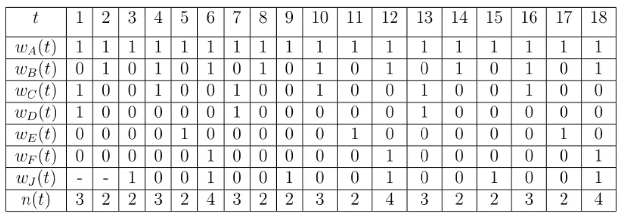
(20) 1 2. t wA (t) wB (t) wC (t) wD (t) wE (t) wF (t) n(t). 1 0 1 1 0 0 3. 1 1 0 0 0 0 2. 3 4 5 1 0 0 0 0 0 1. 1 1 1 0 0 0 3. 1 0 0 0 1 0 2. 6 7 8 1 1 0 0 0 1 3. 1 0 1 1 0 0 3. 1 1 0 0 0 0 2. 9 10 1 0 0 0 0 0 1. 1 1 1 0 0 0 3. 11 12 13 1 0 0 0 1 0 2. 1 1 0 0 0 1 3. 1 0 1 1 0 0 3. 14 15 1 1 0 0 0 0 2. 1 0 0 0 0 0 1. 16 17. 18. 1 0 0 0 1 0 2. 1 1 0 0 0 1 3. 1 1 1 0 0 0 3. Table 3.1: A seuqence of wi (t) and n(t).. the amount of wakeup stations in each beacon slot. We observe the condition that the same sequence between six columns in n(t) raw. We said such a sequence is a pattern. The pattern length, £p , is the least common multiple of the listen interval size, li , of each station. £p = LCM {li } Suppose at time t3 , there is a new station J joins in. The listen interval size of station J is 3. The pattern length may update if listen interval size is not the factor of pattern length. £p = LCM {li , lJ } The status of AP after station J joins in showed in table 3.2.. Then we can see the maximum value of n(t) raw is 4. It means there exists a condition that there are four stations wakeup at the same beacon slot.. But if we let station J wake up at t5 . The status of AP showed in table 3.3.. 17.

(21) 1 2. t wA (t) wB (t) wC (t) wD (t) wE (t) wF (t) wJ (t) n(t). 1 0 1 1 0 0 3. 1 1 0 0 0 0 2. 3 4 5 1 0 0 0 0 0 1 2. 1 1 1 0 0 0 0 3. 1 0 0 0 1 0 0 2. 6 7 8 1 1 0 0 0 1 1 4. 1 0 1 1 0 0 0 3. 1 1 0 0 0 0 0 2. 9 10 1 0 0 0 0 0 1 2. 1 1 1 0 0 0 0 3. 11 12 13 1 0 0 0 1 0 0 2. 1 1 0 0 0 1 1 4. 1 0 1 1 0 0 0 3. 14 15 1 1 0 0 0 0 0 2. 1 0 0 0 0 0 1 2. 16 17. 18. 1 0 0 0 1 0 0 2. 1 1 0 0 0 1 1 4. 1 1 1 0 0 0 0 3. Table 3.2: A sequence of wi (t) and n(t) after station J joins in power saving mode.. 1 2. t wA (t) wB (t) wC (t) wD (t) wE (t) wF (t) wJ (t) n(t). 1 0 1 1 0 0 3. 1 1 0 0 0 0 2. 3 4 5 1 0 0 0 0 0 0 1. 1 1 1 0 0 0 0 3. 1 0 0 0 1 0 1 3. 6 7 8 1 1 0 0 0 1 0 3. 1 0 1 1 0 0 0 3. 1 1 0 0 0 0 1 3. 9 10 1 0 0 0 0 0 0 1. 1 1 1 0 0 0 0 3. 11 12 13 1 0 0 0 1 0 1 3. 1 1 0 0 0 1 0 3. 1 0 1 1 0 0 0 3. 14 15 1 1 0 0 0 0 1 3. 1 0 0 0 0 0 0 1. 16 17. 18. 1 0 0 0 1 0 1 3. 1 1 0 0 0 1 0 3. 1 1 1 0 0 0 0 3. Table 3.3: A sequence of wi (t) and n(t) after station J with first wakeup time t5 .. We can see the maximum value of n(t) raw is 3. It means there exists a condition that there are three stations wakeup at the same beacon slot. By scheduling stations wakeup time, we can reduce the amount of wakeup stations in one beacon slot. We should determine the wakeup time when a new station joins in. Thus, the amount of wakeup stations can be balanced.. So we formulate this problem. We can define a wakeup sequence wi (1), wi (2), ..., wi (k) for station i starting from beacon interval 1 to k. For example, if station 18.

(22) i with li = 4 goes sleeping at beacon interval 0, then its wakeup sequence from beacon interval 1 to 12 is wi (1), wi (2), ..., wi (12) = 000100010001. In general, if a mobile station i with wakeup counter ci (t) and listen interval li at beacon interval t we can find wi (t + k) for beacon interval t + k by (. wi (t + k) =. 1, if k mod li = ci (t) 0, otherwise. Where set S includes all sleeping stations. The problem considered in this paper can be stated as follows: Given a set of sleeping station S at beacon interval t consisting m stations and each of the station i having wakeup counter ci (t) and li , for a new sleeping station j assign an initial value to its cj (t) such that the maximum value of n(t) =. P i∈S∪{j}. wi (t), t = 1, 2, ..., £p is minimized.. The wakeup time of a new station when the station joins in should be determined by AP. AP should calculate the current service status. AP arranges the insertion position of the new station according to its listen interval size. By testing all conditions that less than listen interval value, it can be picked an optimum value such that let the total amount of wakeup stations is minimized.. So we show an example that AP how to determine the wakeup time of a new station J joins in. Suppose a new station J joins the AP at time t3 . AP calculates the table of wakeup stations list in table 3.4. It shows the current service condition in AP. For example, A will wakeup at time t3 . And A, B, C will wakeup at time t4 . The table size is the pattern length because it will repeat.. Because the listen interval size of station J is 3. Thus, the distribution of 19.

(23) Time t3 t4 t5 t6 t7 t8. Wakeup Stations List A A, B, C A, E A, B, F A, C, D A, B. Table 3.4: The wakeup stations of beacon interval t3 to t8 .. wakeup stations we showed as follows. Suppose station J wakeup at t3 , the table is in table 3.5. Maximum amount of wakeup stations is 4. Suppose station J wakeup at t4 , the table is in table 3.6. Maximum amount of wakeup stations is also 4. Suppose station J wakeup at t5 , the table is in table 3.7. Maximum amount of wakeup stations is 3.. Time t3 t4 t5 t6 t7 t8. Wakeup Stations List A, J A, B, C A, E A, B, F, J A, C, D A, B. Table 3.5: The wakeup stations of beacon interval t3 to t8 with station J scheduled in t3 .. Because the condition of station J wakeup at t6 is equal to t3 , we need not calculate that condition. It is the optimal result that station J wakeup at t5 .. Another representation of AP status is that we use wakeup counter to indi20.

(24) Time t3 t4 t5 t6 t7 t8. Wakeup Stations List A A, B, C, J A, E A, B, F A, C, D, J A, B. Table 3.6: The wakeup stations of beacon interval t3 to t8 with station J scheduled in t4 .. Time t3 t4 t5 t6 t7 t8. Wakeup Stations List A A, B, C A, E, J A, B, F A, C, D A, B, J. Table 3.7: The wakeup stations of beacon interval t3 to t8 with station J scheduled in t5 .. cate station wakeup time. We define ci (t) is a counter indicating the amounts of beacon interval until next wakeup time of station i. Each station’s counter will decrease by one after a beacon interval passing. And a mobile station is wakeup if its corresponding counter becomes zero. After that, the counter will reset to its listen interval for further decreasing. Thus, for any given beacon slot t, counter of station i will set as: ci (t) = ci (t − 1) − 1, ci (t) 6= 0 ci (t) = li − 1, ci (t) = 0 Table 3.8 is another representation of original AP service status in wakeup 21.

(25) counter form.. t. 1 2 3. cA (t) 0 cB (t) 1 cC (t) 0 cD (t) 0 cE (t) 4 cF (t) 5 n(t) 3. 0 0 2 5 3 4 2. 0 1 1 4 2 3 1. 4 5 6 0 0 0 3 1 2 3. 0 1 2 2 0 1 2. 0 0 1 1 5 0 3. 7 8 9 0 1 0 0 4 5 3. 0 0 2 5 3 4 2. 0 1 1 4 2 3 1. 10 11 0 0 0 3 1 2 3. 0 1 2 2 0 1 2. 12 13 14 0 0 1 1 5 0 3. 0 1 0 0 4 5 3. 0 0 2 5 3 4 2. 15 16 0 1 1 4 2 3 1. 0 0 0 3 1 2 3. 17 18 0 1 2 2 0 1 2. 0 0 1 1 5 0 3. Table 3.8: To show the current status of the AP in wakeup counter form.. Although the LAWS does reduce the contention pressure between stations, it is still a contention-based media accessing approach. Problem of traffic collision is still existed. For reducing the traffic collision, the Contention Avoidance Traffic Scheduling (CATS) is proposed in the next chapter.. 22.

(26) Chapter 4 Contention Avoidance Traffic Scheduling The goal of CATS is to reduce the contention of stations. In CATS, AP not only setting the TIM bitmap of beacon signal to indicate the wakeup stations but also scheduling the access sequence of these wakeup stations. There are three different access scheduling mechanisms in CATS. In the first mechanism, only one station will be indicated to access the buffered data within each beacon slot. In the second mechanism, multiple wakeup mobile stations are indicated to get back their buffered data. The access sequence is according to their AID. The final mechanism is like the second one but the access sequence is determined by the length of queuing size.. 4.1. Multiple Wakeups Single Access The trivial method to avoid contention between stations is let single station. dominate the whole beacon slot. So the contention for sending PS-Poll frame will be eliminated. In this mechanism, the indicating stations will have their ci (t) = 0. 23.

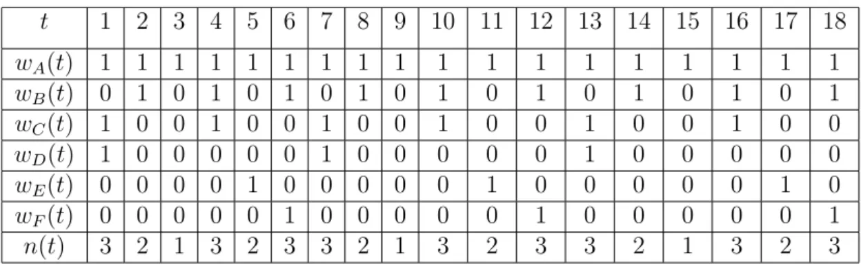
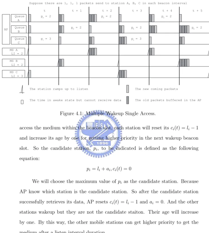
(27) in the lookup table of AP. The candidate wakeup station to be indicated is the one with maximum size of listen-interval. Thus, those long listen-interval stations will have higher chance to retrieve the queuing data and the average queue delay of whole system can decrease. So the candidate station, Spi , to be indicated is defined as the following equation: pi = li , ci (t) = 0 In figure 4.1, There are three mobile stations, Sa , Sb , and Sc , and their corresponding traffic generation rates per beacon are 1, 1, and 1. And the listen interval size of each station is 2, 2 and 3. In the TBTT of beacon slot t, Sa and Sc are wakeup simultaneously and AP indicates station Sc to retrieve its buffered data because lc = 3 is the maximum one. Indications of Sa is delayed to its next wakeup beacon slot. In the beacon slot t + 1, only Sb is wakeup. So Sb is indicated and retrieves its buffered data. In the next beacon slot, t + 2, Sa is wakeup simultaneously. In the beacon slot t + 3, AP finds that pc = 3 is large than pb = 2, so it indicates Sc to retrieve all of the buffered data. For Sb , it will wait until its next wakeup beacon slot.. But if there is a station with small listen interval size in the AP, it may cannot get the medium by the candidate choice equation. For example, a station with listen interval size equals to 1 in figure 4.2. It cannot get the medium because its candidate value always smaller than any station.. Thus, to break draw, each wakeup station i uses an age, ai , to set the priority. At first, the age of each station is set to zero. Because only one wakeup station can 24.

(28) Suppose there are 1, 1, 1 packets send to station A, B, C in each beacon interval t Queue A. AP. t + 1. t + 2. pa = 2. pb = 2. Queue B Queue C. t + 3. pa = 2. t + 4. pb = 2. pc = 3. t + 5. pa = 2. pb = 2. pc = 3. MS A LI = 2 MS B LI = 2 MS C LI = 3. The station ramps up to listen. The new coming packets. The time in awake state but cannot receive data. The old packets buffered in the AP. Figure 4.1: Multiple Wakeup Single Access. access the medium within the beacon slot, each station will reset its ci (t) = li − 1 and increase its age by one for getting higher priority in the next wakeup beacon slot. So the candidate station, pi , to be indicated is defined as the following equation: pi = li + ai , ci (t) = 0 We will choose the maximum value of pi as the candidate station. Because AP know which station is the candidate station. So after the candidate station successfully retrieves its data, AP resets ci (t) = li − 1 and ai = 0. And the other stations wakeup but they are not the candidate staiton. Their age will increase by one. By this way, the other mobile stations can get higher priority to get the medium after a listen interval duration.. If there are more than two stations with the same pi value, we will pick the 25.

(29) Suppose there are 1, 1, 1, 1 packets send to station A, B, C, D in each beacon interval t Queue A. t + 1. pa = 2. Queue B. t + 2. t + 3. t + 4. pb = 2. pb = 3. t + 5. pa = 2. pa = 2. pb = 2. AP Queue C. pc = 3. Queue D. pd = 1. pc = 3 pd = 1. pd = 1. pd = 1. pd = 1. pd = 1. MS A LI = 2 MS B LI = 2 MS C LI = 3 MS D LI = 1. The station ramps up to listen. The new coming packets. The time in awake state but cannot receive data. The old packets buffered in the AP. Figure 4.2: Multiple Wakeup Single Access without age. station with larger listen interval value. If more than two stations with the same listen interval value, we will choose the first station as candidate.. Thus, by using the age, each station can get the medium. The operations showed in figure 4.3. In the beacon time t + 3, pd is larger than other stations. So Sd can have the medium to retrieve data.. 4.2. Multiple Wakeups Multiple Accesses Although the Multiple Wakeups Single Access remove the medium contention,. 26.

(30) Suppose there are 1, 1, 1, 1 packets send to station A, B, C, D in each beacon interval t pa = 2+0 = 2. Queue A. t + 1. t + 2 pa = 2+1 = 3. pb = 2+0 = 2. Queue B AP. pd = 1+0 = 1. Queue D. t + 4 pa = 2+0 = 2. pb = 2+0 = 2. pc = 3+0 = 3. Queue C. t + 3. t + 5. pb = 2+1 = 3. pc = 3+0 = 3 pd = 1+1 = 2. pd = 1+2 = 3. pd = 1+3 = 4. pd = 1+0 = 1. pd = 1+1 = 2. MS A LI = 2 MS B LI = 2 MS C LI = 3 MS D LI = 1. The station ramps up to listen. The new coming packets. The time in awake state but cannot receive data. The old packets buffered in the AP. Figure 4.3: Multiple Wakeup Single Access with age. it is not good in both bandwidth utilization and system throughput. The high queuing latency is its another critical side-effect. To overcome its faults, we release the constraint, single beacon slot single access, and allow more wakeup stations using the same beacon slot. The first encountered problem is how to schedule the access sequence to free the contention. Here we give two methodologies to schedule the access sequences of stations.. 4.2.1. The Smallest AID First. The first methodology we used to free the contention is scheduling the transfer sequence of stations according to their association ID. At first, those stations 27.

(31) that have their ci (t) = 0 and maximum values in li + ai will be indicated in TIM of beacon frame. In order not to change the IEEE 802.11 standard, the access sequence is scheduled by using each station’s AID. The station with small AID will access the medium before the large one. Each station will know what time it will start to retrieve data. By scheduling the sequence, the time wasted in random back-off to send PS-Poll frame can be saved.. Notice that the amounts of total indicated wakeup stations must be controlled according to the summary size of their transmission data. If the summary size of transmission data exceeds the maximum capacity that a beacon slot can afford, some stations will awake whole the beacon slot but do not have the chance to retrieve it data.. In figure 4.4, station Sd which has the same packet generation rate as Sa . Their corresponding AID is 1, 2, 3, and 4. And assume that maximum capacity of transmission packets within a beacon slot is 8. In beacon slot t, all of Sa , Sb , Sc , and Sd are wakeup and indicated to retrieve their data. This is because summation of total transmission packets are 2 + 2 + 1 + 2 = 7 which is not large than capacity of a beacon slot. Their access sequence is Sa , Sb , Sc , and then Sd based on the value of their AID. In beacon t+1, Sb is wakeup and retrieves its data.. In beacon slot t + 2, wakeup stations, Sa , Sb and Sd , are indicated to retrieve their buffered data. For station Sb , because the remaining capacity is not enough for it to retrieve its buffered data, so Sb sets its ab = 1 for higher priority in next wakeup beacon slot. In beacon slot t + 3, Sb and Sc are wakeup and retrieves their 28.

(32) Suppose there are 2, 2, 1, 2 packets send to station A, B, C, D in each beacon interval. Queue A Queue B AP. t pa = 2+0 = 2. t + 1. t + 2 pa = 2+0 = 2. t + 3. t + 4 pa = 2+0 = 2. t + 5. pb = 1+0 = 2. pb = 1+0 = 1. pb = 1+0 = 1. pb = 1+1 = 2. pb = 1+0 = 1. pb = 1+0 = 1. pc = 3+0 = 3. Queue C. pd = 2+0 = 2. Queue D. pc = 3+0 = 3 pd = 2+0 = 2. pd = 2+0 = 2. MS A(1) LI = 2 MS B(2) LI = 1 MS C(3) LI = 3 MS D(4) LI = 2. The station ramps up to listen. The new coming packets. The time in awake state but cannot receive data. The old packets buffered in the AP. Figure 4.4: An example of the smallest AID first method. data.. 4.2.2. The Smallest Queue Length First. The second methodology to free the contention is similar to the previous one. Instead of using AID to schedule the sequence, this method uses the length of packets buffered in the AP. After choosing the candidates, we will sort these stations by buffered data length. The short buffered queue will be arranged at first. If we let these stations with a small buffered data length retrieve data early, they can enter sleeping mode more quickly. Thus, always selecting the station with short buffered queue will increase the average sleep time of every station. 29.

(33) Suppose there are 2, 2, 1 packets send to station A, B, C in each beacon interval. Queue A AP. Queue B Queue C. t pa = 2+0 = 2. t + 1. t + 2 pa = 2+0 = 2. t + 3. t + 4 pa = 2+0 = 2. t + 5. pb = 1+0 = 1. pb = 1+0 = 1. pb = 1+0 = 1. pb = 1+0 = 1. pb = 1+0 = 1. pb = 1+0 = 1. pc = 2+0 = 2. pc = 2+0 = 2. pc = 2+0 = 2. MS A LI = 2 MS B LI = 1 MS C LI = 2. The station ramps up to listen. The new coming packets. The time in awake state but cannot receive data. The old packets buffered in the AP. Figure 4.5: An exmaple of the smallest queue length first method.. Figure 4.5 shows an example of the smallest queue length first method. There are three stations, A, B, and C with listen interval (lA , lB , lC ) = (2, 1, 2) with under the service of an AP. Suppose packet arrival rates of stations A, B, and C are 2, 2, and 1 frames per beacon interval. The maximum size that AP can transfer to stations in a beacon interval is assumed to be 8 frames. In beacon interval t, all of the three stations wakeup. Because the number of buffered frames are 2 + 2 + 1 = 5 (5 < 8), the AP marks AIDs 1, 2, and 3 in the TIM and adds the access sequence C, A, and B in the beacon frame. In beacon interval t + 2, the access sequence is stations C, B, and A. Note that if two stations have same queue length, AP uses their pi to break the tie.. 30.

(34) Chapter 5 Simulation and Results 5.1. Performance Metrics and Environment Setup In this section, we show the performance analysis for the proosed shcemes:. 1. Load-Aware Wakeup Scheduling (LAWS); 2. Multiple Wakeups Single Access (MWSA); 3. Multiple access with the Smallest AID First (SAF); 4. Multiple access with the Smallest Queue Length First (SQLF). The metrics for simulation are given as follows: 1. Average sleeping time of each station: This measure is the duration that a station stays in sleeping mode. If a scheme can make stations stay more time in sleeping, then stations will save more power and operate longer. 2. Average throughput of AP: This value shows the total amount of data successfully transmitting per second. If AP can efficiently schedule and distribute the access of its serving stations, it will have higher data throughput.. 31.

(35) 3. Average latency of a successful transmission: The latency is defined as the time duration starting while a packet is issued and buffered at AP and ending when the target station returns the acknowledge of successful receiving. An AP with well scheduling on stations accessing will make the latency as small as possible. Thus, the resources required for buffering data can be reduced. Our simulation uses an IEEE 802.11b wireless communication module with 11Mbps data rate. The maximum bandwidth for each station is set to 240kbps and an AP can service at most 30 stations. Each station will randomly set 1 to 5 beacon intervals as its listen interval size and its packet arrival rate is 3 packets per beacon interval. Packet size in our simulation is fixed and set to 1KB. Communication channel assumes to be clear and symmetric. The total simulation time is 3 minutes. More simulation configurations such as header length, and inter-frame spaces (IFS) are list in table 5.1. Simulation results will compare the IEEE 802.11 PS mode with the proposed LAWS, MWSA, SAF, and SQLF schemes.. 11Mbps. Data Rates. 28 bytes MAC header 20 bytes IP header 20 bytes UDP header 28 bytes Beacon frame 14 bytes ACK frame 14 bytes PS-Poll frame 0.00001 second SIFS 0.00005 second DIFS 0.00002 second Slot time 0.1 second Beacon interval Table 5.1: Detail simulation configurations.. 32.

(36) 5.2. Results and Discussion Figure 5.1 shows the relation between average sleeping time and number of. stations. Considering contention-based schemes, LAWS can have more sleeping time than IEEE 802.11 PS mode in any size of stations. By using all kinds of MWSA, SAF, and SQLF to reduce the contention within a beacon interval, stations can have more time on staying in sleeping than LAWS and IEEE 802.11 PS mode. In this figure, it seems that MWSA has better sleeping time than both SAF and SQLF. However, we will find in figure 5.3 that it trades the transmission latency with the sleeping time.. The Average Sleeping Time 180. 170. 160. 150. 140 802.11 PSM LAWS MWSA. 130. SAF SQLF 120. 5. 10. 15. 20. 25. 30. Number of Station(s). Figure 5.1: The average sleeping time. Figure 5.2 shows the throughput of AP in delivering buffered packets to sta33.

(37) tions. From this figure, we can explicitly find that the throughput of IEEE 802.11 PS mode falls down quickly when station number is large than 20. However, our proposed schemes, LAWS, MWSA, SAF, and SQLF, are not influenced as number of station increases. This is because our schemes can efficiently avoid the data collision between stations.. 6. 8. The Throughput of Each Scheme. x 10. 802.11 PSM LAWS 7 MWSA SAF SQLF. Throughput(bps). 6. 5. 4. 3. 2. 1. 5. 10. 15. 20. 25. 30. Number of Station(s). Figure 5.2: The throughput of each scheme. In figure 5.3, we show the average latency of a successful transmission for each scheme. For LAWS, SAF, and SQLF, all of their latency is smaller than 0.3 second and increase slowly as number of stations grows. Because only one station is indicated within a beacon interval, the latency of MWSA is longer than the other proposed schemes. While number of station increases, waiting time to deliver the 34.

(38) buffered data will increase. The IEEE 802.11 PS mode, however, will suffer high latency while number of collision packets grows causing by increasing station.. The Latency of Each Scheme 12 802.11 PSM LAWS 10. MWSA SAF SQLF. 8. 6. 4. 2. 0. 5. 10. 15. 20. 25. 30. Number of Station(s). Figure 5.3: The latency of a successful transmission for each scheme. Finally, figure 5.4 shows the improving rate of each proposed schemes in sleeping time (compare with IEEE 802.11 PS mode). By efficiently scheduling the wakeup time of sleeping stations, the sleeping duration of our LAWS, MWSA, SAF, and SQLF schemes can improve explicitly.. 35.

(39) The Sleeping TIme Improving Rate of Each Scheme (Compare to Original Power Saving Mode of IEEE 802.11) 40 LAWS MWSA 35. SAF SQLF. 30. 25. 20. 15. 10. 5. 0. 5. 10. 15. 20. 25. 30. Number of Station(s). Figure 5.4: The improving rate of sleeping time (compared with PS mode of IEEE 802.11).. 36.

(40) Chapter 6 Conclusion and Future Work In this thesis, we proposed a load-aware wakeup scheduling (LAWS) and a contention avoidance traffic scheduling (CATS) for supporting power saving in infrastructure mode in IEEE 802.11 standard. Our methods need not to modify IEEE 802.11 standard and can apply for current circumstance. We can see that the average station sleeping time improved when using the LAWS. By using the CATS the average station sleeping time can be increased when comparing to original power saving mode.. The key point of this thesis focuses on traffic scheduling concept. Our methods explicitly save the stations’ power which are operating in infrastructure mode. We can balance the amount of wakeup stations and schedule the access sequence of stations by setting the TIM efficiently. In our schemes, the beacon interval is not dynamically modified so that the stations in infrastructure mode of IEEE 802.11 can operate as the original one. The only one which needs to be modified is Access Point. In other words, our schemes can compatible to the original IEEE 802.11 WLANs.. 37.

(41) In our thesis, our proposed LAWS do not work well if the AP starts with multiple serviced stations which are not scheduled by using LAWS. Thus, if the LWAS can periodically re-schedule the wakeup time of each serviced station to make all beacon interval a balancing amount of wakeup stations, the LAWS will approximate the optimal scheduling solution for all of the serviced station. And this is the future work on which we will make our effort.. 38.

(42) Bibliography [1] IEEE 802.11 Working Group. Wireless LAN Medium Access Control (MAC) and Physical Layer (PHY) Specifications, 1999 [2] IEEE 802.11 Working Group. Wireless LAN Medium Access Control (MAC) and Physical Layer (PHY) Specifications: High-speed Physical Layer in the 5GHz Band, 1999 [3] IEEE 802.11 Working Group. Wireless LAN Medium Access Control (MAC) and Physical Layer (PHY) Specifications: Higher-speed Physical Layer Extension in the 2.4GHz Band, 1999 [4] Specification Documents. [Online] http://www.bluetooth.org/spec/ [5] 3GPP Specifications Home Page. [Online] http://www.3gpp.org/specs/ specs.htm [6] C. Jones, K. Sivalingam, P. Agrawal, and J. Chen, ”A Survey of Energy Efficient Network Protocols for Wireless Networks”, In ACM Journal of Wireless Networks (WINET), Vol 7, Issue 4, pp. 343-358, Aug, 2001. [7] T. Simunic, L. Benini, P. Glynn, and G. De Micheli , ”Dynamic Power Management for Portable Systems”, In Proceedings of the 6th annual international. 39.

(43) conference on Mobile computing and networking (IEEE MobiCom), Boston, Massachusetts, USA, pp. 11-19, 2000. [8] R. Kravets, and P. Krishnan, ”Application-Driven Power Management for Mobile Communication”, InWireless Networks Volume 6, Issue 4, pp. 263277, July, 2000. [9] L. Marie Feeney, and M. Nilsson, ”Investigating the Energy Consumption of a Wireless Network Interface in an Ad Hoc Networking Environment”, In Proceedings of IEEE Conference on Computer Communications (IEEE InfoCom), Anchorage Alaska, USA, pp. 1548-1557, Apr, 2001. [10] E. Shih, P. Bahl, and M. J. Sinclair, ”Wake on Wireless: An Event Driven Energy Saving Strategy for Battery Operated Devices”, In Proceedings of the 8th annual international conference on Mobile computing and networking (IEEE MobiCom), Atlanta, Georgia, USA, pp. 160-171, Sep, 2002. [11] R. Krashinsky, and H. Balakrishnan, ”Minimizing Energy for Wireless Web Access with Bounded Slowdown”, InProceedings of the 8th annual international conference on Mobile computing and networking, Atlanta, Georgia, USA, pp. 119-130 Sep 23-28, 2002. [12] A. Sheth, and R. Han, ”Adaptive Power Control and Selective Radio Activation For Low-Power Infrastructure-Mode 802.11 LANs”, In Proceedings of 23rd International Conference on Distributed Computing Systems Workshops (ICDCSW’03, Providence, Rhode Island, USA, pp. 812-817, May 19-22, 2003. [13] J.R. Jiang, Y.C. Tseng, C.S. Hsu, and T.H. Lai, ”Quorum-Based Asynchronous Power-Saving Protocols for IEEE 802.11 Ad Hoc Networks”, In Pro40.

(44) ceedings of International Conference on Parallel Processing, Nice, France, pp. 812-817, April 22-26, 2003. [14] J.R. Jiang, Y.C. Tseng, C.S. Hsu, and T.H. Lai, ”Quorum-Based Asynchronous Power-Saving Protocols for IEEE 802.11 Ad Hoc Networks”, ACM Mobile Networking and Applications (MONET), special issue on Algorithmic Solutions for Wireless, Mobile, Ad Hoc and Sensor Networks, Vol. 10, No. 1/2, pp. 169-181, 2005. [15] J. Lorchat, and T. Noel, ”Energy Saving in IEEE 802.11 Communications using Frame Aggregation”, IEEE Global Communication Conference (GLOBECOM’ 03), San Francisco, USA, Dec, 2003. [16] Y. Agarwal, C. Schurgers, and R. Gupta, ”Dynamic Power Management using On Demand Paging for Networked Embedded Systems”, Asia South Pacific Design Automation Conference (ASP-DAC’05), Shanghai, China, pp. 755759, Jan 18-21, 2005. [17] C. S. Raghavendra, and S. Singh, ”PAMAS - Power Aware Multi-Access Protocol with Signalling for Ad Hoc Networks”, ACM SIGCOMM Computer Communication Review Volume 28, Issue 3, pp. 5-26, July, 1998. [18] M. Liu, and M. T. Liu, ”A Power Saving Scheduling for IEEE 802.11 Mobile Ad Hoc Network”, In Proceedings of International Conference on Computer Networks and Mobile Computing (ICCNMC’03), Shanghai, China, pp. 238245, Oct 20-23, 2003.. 41.

(45)