Analyzing Ordinal Data for Group Representation
WAY C.W. CHANG,* PO-YOUNG CHU, CHERNG G. DING, SOUSHAN WU
Institute of Business and Management, College of Management, National Chiao-Tung University, No. 114, 4th Floor, Section 1, Chung Hsiao West Road, Taipei, Taiwan
Abstract
With n individuals ranking m objects, the exhaustive comparison approach, proposed in this paper, produces a list of order vectors sorted by the relative number of concordant pairs. The exhaustive comparison approach compares all possible order vectors instead of “an” optimal order vector to help the data analyst to consider “practical” solutions rather than a “desired” solution. An overall concordant order ratio is proposed to measure “how well” each order vector may represent the ranking structure of an ordinal data set. And the marginal concordant ratio evaluating the goodness of fit of each object in each order vector is also proposed in this paper. Comparisons among some popular ranking methods are discussed in this article. An empirical survey data regarding how travelers considered various factors for choosing travelling locations are used to illustrate the proposed method and calculations.
Key words: distance-based ranking methods, exhaustive comparison approach, marginal order ratio, overall concordant order ratio, overall ranking
1. Introduction
The purpose of overall ranking is to find an order vector consisting of the ranks of objects to represent the ordinal information of an ordinal data set. When a dominant order pattern can be found in an ordinal data set, the ordinal relationships in the ordinal data set can be summarized with an order vector. When the order structure is complicated, an order vector is not sufficient to describe the ranking structure, and the overall ranking may only provide limited ranking information. It is useful to know “how well” an order vector may be used to represent the ranking structure of an ordinal data set. In addition, it is also useful to know the goodness of fit of each object in the overall order vector, because there may be some objects in the overall order vector fit their ranking positions better than other objects.
This article attempts to propose a measurement of the overall fit of an order vector to represent the ranking structure of the ordinal data set. The goodness of fit of each object in the overall order vector will also be proposed and discussed. A numerical example about how travellers considered various factors for choosing travelling locations will be used to illustrate the proposed method and calculations.
*The authors are listed in alphabetical order. Correspondence author: Way Chang, e-mail: wchang@sunwk1.tpe.nctu.edu.tw
2. Overall ranking formulation
The overall ranking problem can be formulated as that m objects are presented to n judges for ranking and an order vector consisting of m objects will be derived from these n ranking. An order vector is composed of objects listed from the most important to the least important. For example, five objects (A, B, C, D, E) are presented to judges J1, J2 and J3 for ranking. Judge 3 may consider A < C < D < E < B, and his order vector will be J3 (A < C < D < E < B). A rank vector can be derived from the order vector by assigning the position number in the order vector to each factor. The rank vector for judge 3 will be J3 (1A, 5B, 2C, 3D, 4E) or J3 (1, 5, 2, 3, 4) in brief. Order vector contains the names of objects in preference sequence, while rank vector contains the rank values of objects in object sequence. Rank values will be used for computation purposes and object names will be used for description purposes in this article.
The overall ranking derived from an ordinal data set may serve two purposes: 1. ranking for group consensus, and
2. ranking for group representation.
Ranking for group consensus is to derive a unanimous order vector acceptable by most of the members in the related group. Group consensus is needed in many occasions; such as, ranking products and selecting the best product, sport competitions, public policy hearing, etc. Consumers and producers must have certain agreement about the product ranking in order to make the ranking meaningful and useful. Procedures and methods, such as multiple-stage evaluations, repeated rating, round robin tournaments, majority votes, jury verdict, Delphi method . . . can be used to derive group consensus to result in group consensus. The derivation and acceptance of group consensus is very complicated and beyond the scope of the article.
Ranking for group representation is to evaluate how well an order vector may represent an ordinal data set. In a consumer taste survey, it would be interesting to know the number of dominant taste patterns and their representativeness among various consumer groups. The purpose of consumer survey is to study taste patterns and their corresponding degrees of concentration instead of developing group consensus.
This article will discuss the group ranking for representation problem, but will not address the existence or the determination of group consensus problem. The purpose of group representation is to measure the representativeness of a ranking pattern rather than to develop an order vector for group consensus. Measurements of group ranking for representation may provide supplementary information in determining group consensus.
3. Literature review
Many papers have been written discussing the methods of obtaining an overall order vector or measuring the strength of the ordinal association between an order vector and the rank data. However, little attention has been paid to the group representation problem. Literature
concerning the overall ranking problem can be traced as far back as centuries ago (Borda 1781; Fechner 1860). Summaries of various ordinal-ranking methods can be found in the literature (Cook, Kress and Seiford 1997; Kruskal 1958; Lansdowne 1996; Marden 1995). A simple and popular overall ranking method proposed by Borda used the sums (or the averages) of rank values to determine an overall order vector. Other methods utilize distance functions to measure the dispersion of rank vector y about a given rank vector yvto find
the shortest-distance rank vector. Two kinds of distances, spatial and disorder distances, are often used to model the dispersion between y and yv. The spatial distance measures the differences of rank values between two rank vectors. The disorder distance measures the number of disordered pairs between two rank vectors. A desired overall rank vector will be chosen to summarize ordinal data so that the total dispersion may be minimized (Diaconis 1988; Lansdowne 1996; Marden 1995).
Consider the situation of m objects and n judges. Let yi be the rank value of the ith object of y. Several popular distances are summarized in Table 1.
The Spearman’s Footrule (Footrule hereafter) distance is the summation of the absolute rank differences of two rank vectors. The Spearman distance is the square of the Euclidean distance. The Hamming distance summarizes the number of objects having different rank values in two rank vectors. The Kendall distance summarizes the number of discordant pairs from pair-wise comparisons between two rank vectors.
The number of minimum-distance rank vectors can be one or more. Marden (1995, p. 29) proved that if the means of objects yj’s are distinct, then the minimum-Spearman-distance rank vector is unique and is equal to the rank of yj; and the Borda method and the Spearman method will determine identical optimal rank vectors. Cook and Seiford (1978) showed that minimizing the Footrule distance could be formulated as a linear assignment problem. If the medians of objects yimed’s are distinct, then the unique optimal rank vector is equal to
the rank of yimed. When the modes of objects y i
mod’s are distinct, it is obvious that the unique
optimal vector is equal to the rank of yimod.
4. Problems in overall ranking
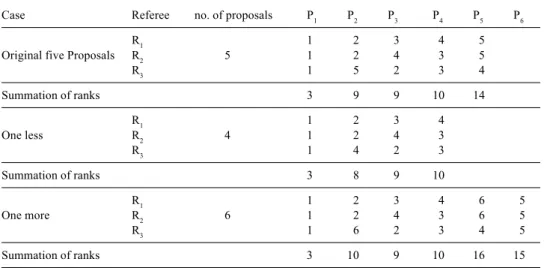
Consider the following hypothetical numerical illustration: (1) three referees (R1, R2, R3) were asked to evaluate the quality of five proposals (P1, P2, P3, P4, P5) for sponsorial fund allocation; (2) P5 is withdrawn and four proposals are retained for evaluation, and (3) a
Table 1. Distance functions Spatial distance dp(y, yv) = Σ 1≤i≤m | yi–yi v | p, Spearmans Footrule (P = 1) Spearman (P = 2) Disorder distance
dHam(y, yv) = #{i | y
i = yi
v, 1≤i≤m}, Hamming distance
dKen(y, yv) = ΣΣ
i≤j≤m I[(yi–yj) (yi v–y
j
v) < 0], Kendall distance
new proposal P6 is submitted for evaluation and all three referees rank it as the fifth preferred proposal. The relative ranks of P1, P2, P3 and P4 should remain the same when one proposal is withdrawn or added to the original ranking as displayed in Table 2.
It is reasonable to expect that adding or removing objects would change the object rank values but should not change the relative positions in the optimal overall rank vectors. Table 3 shows that the optimal order vectors determined by the Borda, Spearman, Footrule, Hamming, and Kendall methods. In the five and the six proposal cases, there are two optimal order vectors under the Borda, Spearman, and Footrule methods. In the four-proposal case, P5 and P6 are removed and the relative ranks of P1, P2, P3 and P4 remain the same. The relative positions of P1, P2, P3 and P4 in the optimal order vectors are different from their relative positions in the five and six proposal cases if the Borda, Spearman and Footrule methods are used. The relative positions of P1, P2, P3 and P4 in the optimal order vectors remain the same under the Hamming and the Kendall methods no matter how many proposals are considered in the hypothetical example.
The Hamming method determined consistent relative positions in the optimal rank vectors in this example. However; the P4 > P5 relationship determined in the optimal rank vectors is not reasonable because two referees (R2 and R3) preferred P5 > P4 and only one referee preferred P4 > P5 in this example. The minority should not have dominant power to overrule the decisions of the majority. The Kendall method utilizes the relative order relationships instead of the rank values, therefore, adding or removing evaluated items will not change the relative positions in the optimal overall rank vectors. In fact, the Kendall pair-wise comparisons are invariant to any monotonic transformation of rank values, because only relative order directions are used instead of their rank values.
It is also reasonable to expect that the largest-distance vectors are the reverse vectors of the least-distance rank vectors. In the example, the largest-distance rank vectors are not the reversed vectors of the least-distance rank vector determined by the Spearman, Footrule, and Hamming methods as displayed in Appendix 1. The smallest and the largest Kendall
Table 2. Ranking lists of three referees
Case Referee no. of proposals P1 P2 P3 P4 P5 P6
R1 1 2 3 4 5
Original five Proposals R2 5 1 2 4 3 5
R3 1 5 2 3 4 Summation of ranks 3 9 9 10 14 R1 1 2 3 4 One less R2 4 1 2 4 3 R3 1 4 2 3 Summation of ranks 3 8 9 10 R1 1 2 3 4 6 5 One more R2 6 1 2 4 3 6 5 R3 1 6 2 3 4 5 Summation of ranks 3 10 9 10 16 15
distance vectors must be symmetrically reversed because the Kendall distance of a reversed order vector is equal to a constant (total number of comparisons minus the original distance). It seems that the Kendall method yields a more consistent and desirable overall ranking than other methods in the hypothetical example.
In addition, it is reasonable to expect that the optimal order vector would be different when a change occurs in the rank data set. The ordinal data set can be viewed as a large data matrix consisting of m object columns and n observation rows. Swapping cells in the same column will not change the optimal order vectors under the Borda, Spearman, Footrule, and Hamming methods, because only column values instead of row relationships are used in determining the optimal rank vector. Such swaps will change the original ranking relationships in the row vectors, but the optimal rank vector remains unaffected. The Kendall optimal order vectors will be affected whenever the row relationships are changed.
From the previous numerical illustration, we need to avoid at least three situations in determining the “optimal” overall order vectors:
• No minority order relationships should be dominant in determining the optimal overall order vector.
Table 3. Optimal rank vectors of different distance methods and number of proposals
Method No. of proposals Distance P1 P2 P3 P4 P5 P6
Borda 4 N.A. 1 2 3 4 5 N.A. 1 2 3 4 5 N.A. 1 3 2 4 5 6 N.A. 1 3 2 4 6 5 N.A. 1 4 2 3 6 5 Spearman 4 8 1 2 3 4 5 14 1 2 3 4 5 14 1 3 2 4 5 6 22 1 3 2 4 6 5 22 1 3 4 2 6 5 Footrule 4 6 1 2 3 4 6 1 2 4 3 5 8 1 2 3 4 5 8 1 2 4 3 5 6 10 1 2 3 4 6 5 10 1 2 4 3 6 5 Hamming 4 4 1 2 4 3 5 5 1 2 4 3 5 6 5 1 2 4 3 6 5 Kendall 4 3 1 2 3 4 5 4 1 2 3 4 5 6 6 1 2 3 4 6 5
• Relative orders of objects should be consistently retained in a subset in determining the optimal overall order vector.
• The optimal order vector should be sensitive to the change of the ordinal data set. Other criteria for assessing rank models can be found in the literature (Diaconis 1988; Kendall and Lansdowne 1996; Marden 1995; Smith and Babinton 1940).
5. The exhaustive comparison approach
Kendall (1940) proposed a pair-wise approach to compare all rank data against a specific rank vector. The specific rank vector defines all pair-wise relationships for object comparisons. There are at least three advantages using this approach. First, Kendall’s approach only concerns the order direction of objects instead of the magnitude of rank values, which may avoid the criticism of interval assumption about rank values. Second, each observation may equally influence the Kendall distance up to the number of pair-wise comparisons, which eliminates the dominant minority problem. Finally, Kendall’s approach retains consistent subset ranking because the order directions remain the same no matter whether a subset or the full set of objects is considered.
Consider the five proposals case in Table 2. Using Kendall’s approach, the pair-wise comparisons may be conducted as follows: First, select an arbitrary rank vector, say N(1N1 > 2N2 > 3N3 > 4N4 5N5), as a norm vector. Then, comparing any 2 objects out of 5 objects which is to compare 10 (C(5 2) = 5!/(5–2)!/2!) pair-wise order directions between the norm vector and the rank data. For the first referee R1, all 10 pair-wise order directions are concordant, i.e., N(1N1 < 2N2) and R1(1P1 < 2P2); N(1N1 < 3N3) and R1(1P1 < 3P3) . . . N(4N4 < 5N5) and R1(4P4 < 5P5). The norm vector accounts for 100% (or 10/10) of R1’s ranking. For the second referee R2, all order directions are concordant except that N(3N3 < 4N4) but R2(4P3 > 3P4). The norm vector accounts for 90% (9/10) of R2’s ranking. Similarly, the norm vector accounts for 70% (7/10) of R3’S ranking; discordant pairs are: R3(5P2 > 2P3), R3(5P2 > 3P4), and R3(5P2 > 4P5). The norm vector accounts for 86.67%, (100% + 90% + 70%)/3, of the order relationships for the three referees on average. The overall concordant order ratio is defined as the total number of concordant pairs divided by the total number of pair-wise comparisons. The concordant order ratio can be used as a measure of how well the norm vector can be used to represent the order structure of the entire rank data.
Let yv be the vth norm vector of m objects, P be the total number of concordant pairs
between the norm vector yv and n rank data, and Q be the total number of discordant
pairs.
If the rank values of all rank vectors are distinct, then (P+Q) = n×C(m, 2), and Q = n×C(m,2) – P. Define Pv = ΣΣ i≤j≤m I[ (yi v–y j v)(y i–yj) > 0], P
Define the overall concordant order ratio (or order ratio in brief): Rv = Pv / [ P+Qv ] or Rv = Pv / [ n×Q(m,2) ]
The overall concordant order ratio Rv measures the average order percentage accounted
for by the norm vector yv for a given set of rank data, and 0 ≤ Rv ≤ 1. The higher the Rv is,
the better the norm vector may represent the rank data.
The exhaustive approach is to compute the average concordant order ratios for all possible distinct vectors. All possible 120 (5!) distinct norm vectors for the five-proposal case will be sorted according to their descending concordant order ratios. The sorted vector list displays the “optimal” to the “worst” vectors for representing the rank data. The reason to provide many order vectors instead of one optimal order vector is to provide additional alternatives to represent the rank data. In reality, the desired rank pattern might not be a feasible solution for implementation. A full list may facilitate planner to consider the second best or the third best order vectors. And our purpose is to study the representativeness of an overall vector whether it is optimal or not.
The number of marginal concordant pairs, denoted by MPv
i can be computed from a
subset of objects by including only the concordant pairs with the ith object in the order pairs. MPvi will be the marginal contribution from the ith object to Pv. The marginal order
ratio for the ith object is defined as: MRv i = MP
v
i /(m–1)/n, 0 ≤ MR v
i≤ 100%. The (m–1) in the
denominator is equal to the difference between C(m, 2) and C(m–1, 2). It can be further proved that the overall order ratio is equal to the average of m marginal order ratios, i.e., Rv
= Σi =1,m MRv
i / m (c.f. Appendix 2). The marginal order ratio MR v
i measures how well the ith
object of the rank data would fit its corresponding overall ranking position. It provides additional information about the goodness of fit of each object in the overall ranking.
The order ratio is similar to three popular statistics using concordant P and discordant Q, i.e., Kendall’s tau; (P–Q) / (n(n–1)), Goodman and Kruskal’s gamma; (P–Q) / (P+Q), and Somers’s d; (P–Q) / (P+Q+Y0) – Y0 is equal to the number of observations tied on rank data. These statistics are used to measure the ordinal association in the statistics literature. It is easy to show that if P > Q, then the ordinal association coefficients will be positive and Rv >50%. If P < Q, the ordinal association coefficients will be negative and Rv < 50%.
The order ratio Rv defined in this article is quite similar to the Goodman and Kruskal’s
gamma. In fact, the Goodman and Kruskal’s gamma is equal to 2Rv–1. The reason for using
the order ratio rather than the Goodman and Kruskal’s gamma is measuring the overall order structure “accounted” by the rank vector instead measuring the “direction” of association between the rank vector and rank data. Only P is needed to represent the explained order pairs. The difference of P and Q in the Goodman and Kruskal’s gamma is useful to define the direction of the ordinal association, which is not the interest of the ordinal representation study. When the Goodman and Kruskal’s gamma is negative, it is still possible to find some concordant order pairs between the norm vector and the rank data. The magnitude of the order ratio can still measure the portion that has been accounted for by the rank vector. Moreover, the negative Goodman and Kruskal’s gamma cannot clearly reveal the explained portion.
Pair-wise comparisons between n rank data and m! vectors require a lot of computation. C(m,2) times pair-wise comparisons are needed between each observation and the norm
vector. The comparisons may be simplified by constructing an overall pair-wise comparison matrix. The cell value defined in the comparison matrix contains the frequency of observations and the percentage to the total number of observations. Table 4 is an overall pair-wise comparison matrix of the rank data in Table 2. All three referees agreed that P1 < P2; therefore, the cell count is equal to 3 and its percentage is equal to 100% (3/3). We may use the overall pair-wise comparison matrix to compare the number of concordant pairs between a norm vector and the rank data. If the norm vector shows P1 < P2, then we may add the cell count to the concordant-pair total. If the norm vector shows P1 > P2, then we may add the total number of observation minus the cell frequency (3–3 = 0 in this example) to the concordant-pair total. The pair-wise comparisons for each norm vector may be reduced from n × C(m, 2) to C(m, 2) comparisons. The summation of all cell frequencies is equal to the total number of concordant pairs for the norm vector N(1N1 < 2N2 < 3N3 < 4N4 < 5N5) (26 in this example). The average of all cell percentages is equal to the order ratio for N(1N1 < 2N2 < 3N3 < 4N4 < 5N5) (86.67% in this example).
For each vector yv, there must exist a reversed vector yv. It can be shown that P’ = n × C(m, 2) – Pv. We only need to compare the rank data with half of the m! distinct vectors.
The reversed vector of the optimal vector should have the greatest distance because the optimal vector has the smallest distance.
Table 5 displays the two best order vectors determined by the exhaustive comparison approach for the rank data in Table 2. For the five proposals case, the exhaustive comparison approach determines “P1 < P2 < P3 < P4 < P5” being the “optimal” overall order vector with an order ratio 86.67%. It can be seen that P1 has the greatest marginal order ratio 100%.
Table 4. Overall pair-wise comparison matrix of the rank data in Table 2
Row < Col P2 P3 P4 P5
Frequency % Frequency % Frequency % Frequency %
P1 3 100 3 100 3 100 3 100
P2 2 66.7 2 66.7 2 66.7
P3 2 66.7 3 100
P4 3 100
Table 5. Overall order vectors derived from the exhaustive comparison approach
No. Order vector R P P1 P2 P3 P4 P5 P6 MR1 MR2 MR3 MR4 MR5 MR6
l < 2 < 3 < 4 < 5 86.67% 26 1 2 3 4 5 100% 75.00% 83.33% 83.33% 91.67% 5 1 < 2 < 4 < 3 < 5 83.33% 25 1 2 4 3 5 100% 75.00% 75.00% 75.00% 91.67% 1 < 3 < 2 < 4 < 5 83.33% 25 1 3 2 4 5 100% 66.67% 75.00% 83.33% 91.67% 1 < 2 < 3 < 4 83.33% 15 1 2 3 4 100% 77.78% 77.78% 77.78% 4 1 < 2 < 4 < 3 77.78% 14 1 2 4 3 100% 77.78% 66.67% 66.67% 1 < 3 < 2 < 4 77.78% 14 1 3 2 4 100% 66.67% 66.67% 77.78% 1 < 2 < 3 < 4 < 6 < 5 86.67% 39 1 2 3 4 6 5 100% 73.33% 86.67% 86.67% 86.67% 86.67% 1 < 2 < 3 < 4 < 5 < 6 84.44% 38 1 2 3 4 5 6 100% 73.33% 86.67% 86.67% 80.00% 80.00% 6 l < 2 < 4 < 3 < 6 < 5 84.44% 38 1 2 4 3 6 5 100% 73.33% 80.00% 80.00% 86.67% 86.67% 1 < 3 < 2 < 4 < 6 < 5 84.44% 38 1 3 2 4 6 5 100% 66.67% 80.00% 86.67% 86.67% 86.67%
This is not surprising because all three referees ranked P1 the number one proposal. Table 5 shows that P5 has the second largest goodness of fit at the 5th position greater than P
3 at
the 3rd position and P
4 at the 4
th position. P
2 has the least marginal order ratio, indicating
that three referees had quite diversified ranking about P2 at the 2nd position. For the six
proposals case, all three referees ranked P6 being the 5th proposal, but the marginal order
ratio for P6 is not 100%. Table 2 shows that there are two discordant pairs, R3(P6 < P2) and R3(P6 > P5), for P5 between the rank vector and rank data. The marginal order ratio is equal to 10/12 or 86.67% for P5. The marginal order ratio not only evaluates the goodness of fit between object rank values to its overall rank value, but also the goodness of fit among object orders. The goodness of marginal fit is conditioned on the corresponding rank vector instead of the rank values themselves.
The pair-wise comparison matrix can be used to examine if more than 50% of rank data satisfies the overall order relationships defined in the overall order vector. Table 4 displays all pair-wise relationships defined by the P1 < P2 < P3 < P4 < P5 order vector. When all cells in the comparison matrix are no less than 50%, the overall rankings satisfy the Condorcet rule (a social choice function such that the social choice beats or ties all other alternatives in paired comparisons; Riker 1982, p. 293). This overall vector would have the largest number of concordant pairs. If any other order vector is used to define the order system, at least one cell percentage will below 50% and swapping the two comparison items may increase the order ratio. It is reasonable to conclude that there will be no other order vector better representing the order structure of the rank data.
The summation of all frequencies in the comparison matrix is equal to the number of concordant pairs for the optimal order vector, i.e., 6 × 3 + 4 × 2 = 26. The average of all percentages in the comparison matrix is equal to the overall order ratio, i.e., (6 × 100% + 4 × 66.7%) / 10 = 86.67%. The comparison matrix can be used as an alternative interpretation of the overall order ratio.
6. Numerical example
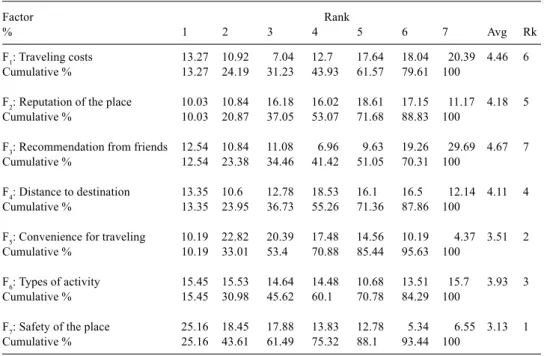
A tourist survey (1996) had been conducted to explore the importance of factors considered in choosing traveling places. Seven factors including: F1 traveling costs, F2 reputation of the place, F3 recommendation from friends, F4 distance to destination, F5 traveling convenience, F6 types of activity, and F7 safety of the place were printed in a questionnaire. People were asked to rank these factors with number 1–7 to reflect how their relative importance in choosing a traveling place and there were 1236 valid replies. The lower the rank is, the more important is the factor in choosing a traveling place. No ties or missing items were allowed to force the evaluators to rank all factors. Table 6 shows the detailed rank distributions and the cumulative distributions of all seven factors. It seems reasonable to expect F7 being the most important object in the optimal vector because the greatest number of observations agreed so. The cumulative distribution of the first three most important factors also confirms F7 being the most important object (61%.> 46% . . .).
The Borda, Footrule and Spearman methods all determine “F7 < F5 < F6 < F4 < F2 < F1 < F3” being the “optimal” order vector. F7 is the most important factor as expected from
Table 6. Distributions of traveling consideration factors
Factor Rank
% 1 2 3 4 5 6 7 Avg Rk
F1: Traveling costs 13.27 10.92 7.04 12.7 17.64 18.04 20.39 4.46 6
Cumulative % 13.27 24.19 31.23 43.93 61.57 79.61 100
F2: Reputation of the place 10.03 10.84 16.18 16.02 18.61 17.15 11.17 4.18 5
Cumulative % 10.03 20.87 37.05 53.07 71.68 88.83 100
F3: Recommendation from friends 12.54 10.84 11.08 6.96 9.63 19.26 29.69 4.67 7
Cumulative % 12.54 23.38 34.46 41.42 51.05 70.31 100
F4: Distance to destination 13.35 10.6 12.78 18.53 16.1 16.5 12.14 4.11 4
Cumulative % 13.35 23.95 36.73 55.26 71.36 87.86 100
F5: Convenience for traveling 10.19 22.82 20.39 17.48 14.56 10.19 4.37 3.51 2
Cumulative % 10.19 33.01 53.4 70.88 85.44 95.63 100
F6: Types of activity 15.45 15.53 14.64 14.48 10.68 13.51 15.7 3.93 3
Cumulative % 15.45 30.98 45.62 60.1 70.78 84.29 100
F7: Safety of the place 25.16 18.45 17.88 13.83 12.78 5.34 6.55 3.13 1
Cumulative % 25.16 43.61 61.49 75.32 88.1 93.44 100
Table 7. Order vectors sorted by descending R
Seq Order vector R P Mr1 Mr2 Mr3 Mr4 Mr5 Mr6 Mr7
1 6<7<5<2<4<1<3 64.34% 16700 65.90% 68.61% 61.14% 67.26% 68.77% 51.21% 67.49% 2 7<5<2<4<1<3<6 63.65% 16520 67.25% 66.21% 63.73% 67.80% 67.23% 48.79% 64.52% 3 7<6<5<2<4<1<3 63.49% 16480 65.90% 68.61% 61.14% 67.26% 68.77% 48.25% 64.52% 4 7<5<6<2<4<1<3 63.05% 16366 65.90% 68.61% 61.14% 67.26% 67.23% 46.71% 64.52% 5 7<5<2<4<1<6<3 62.91% 16328 67.25% 66.21% 61.14% 67.80% 67.23% 46.20% 64.52% 6 6<7<5<4<2<1<3 62.53% 16230 65.90% 62.27% 61.14% 60.92% 68.77% 51.21% 67.49% 7 7<5<2<4<6<1<3 62.52% 16228 65.90% 66.21% 61.14% 67.80% 67.23% 44.85% 64.52% 8 7<5<2<6<4<1<3 62.37% 16188 65.90% 66.21% 61.14% 67.26% 67.23% 44.31% 64.52% 9 6<7<5<2<4<3<1 62.00% 16092 57.70% 68.61% 52.94% 67.26% 68.77% 51.21% 67.49% 10 6<7<5<2<1<4<3 61.85% 16054 57.19% 68.61% 61.14% 58.55% 68.77% 51.21% 67.49% 11 7<5<4<2<1<3<6 61.84% 16050 67.25% 59.87% 63.73% 61.46% 67.23% 48.79% 64.52% 12 6<5<7<2<4<1<3 61.73% 16022 65.90% 68.61% 61.14% 67.26% 59.63% 51.21% 58.35% 13 7<6<5<4<2<1<3 61.68% 16010 65.90% 62.27% 61.14% 60.92% 68.77% 48.25% 64.52% 14 6<7<2<5<4<1<3 61.57% 15980 65.90% 58.90% 61.14% 67.26% 59.06% 51.21% 67.49% 15 7<5<4<6<2<1<3 61.40% 15936 65.90% 62.27% 61.14% 61.46% 67.23% 47.25% 64.52% 16 7<5<2<4<3<1<6 61.30% 15912 59.05% 66.21% 55.53% 67.80% 67.23% 48.79% 64.52% 17 5<6<7<2<4<1<3 61.29% 15908 65.90% 68.61% 61.14% 67.26% 58.09% 49.68% 58.35% 18 7<5<6<4<2<1<3 61.24% 15896 65.90% 62.27% 61.14% 60.92% 67.23% 46.71% 64.52% 19 7<5<2<1<4<3<6 61.16% 15874 58.54% 66.21% 63.73% 59.09% 67.23% 48.79% 64.52% 20 7<6<5<2<4<3<1 61.15% 15872 57.70% 68.61% 52.94% 67.26% 68.77% 48.25% 64.52%
looking up Table 6. Table 7 lists the top 20 sorted order vectors determined by the exhaustive approach and “F6 < F7 < F5 < F2 < F4 < F1 < F3” is the “optimal” order vector. Two optimal order vectors derived by the Borda and exhaustive approach has different order positions for F6 and F2. The most important factor determined by the exhaustive comparison approach is F6 instead of F7; moreover, F6 changes its position in the top 5 order vectors. We might suspect that the exhaustive comparison approach might yield unstable overall ranking.
Table 8 displays the comparison matrix for the traveling data. F6 has circular ordinal relationships with F5 and F2, i.e., F6 < F5, and F5 < F2, but F6 > F2. F6 also violates the transitivity law with F1 and F3. In fact, there is no proper place for F6 to fulfill the transitivity law. If we look up Table 6 again, we can find that F6 is evenly distributed over the 1–7 ranks. F6 does not dominantly occur at any particular ranking. Table 8 shows that more people considered that F6 was more important than F7 in their factor ranking. Positioning F6 before F7 will receive least damage to all other overall ranking. Placing F6 at the first place of the overall order vector does not imply that F6 is the most important factor. It simply indicates that the best-fit position for F6 will be the first position after considering all other factors. “F6 the type of activity” changes its position in the top 5 order vectors. It may have a very vague role in choosing traveling places, which also confirms that F6 provides little information in the overall ranking. If F6 is removed from the comparison matrix, the relationships of the remaining 6 factors conform to the Condorcet rule and the transitivity law. The exhaustive comparison approach provides an opportunity to detect whether F6 is informative or not in determining the overall order vector.
When, F6 is removed from the 7 factors, Table 9 displays a stable order structure for the remaining 6 factors. The “optimal” order vector becomes “F7 < F5 < F2 < F4 < F1 < F3”, the same as determined by the Footrule method, and its R ratio has been increased from 64.35% to 69.59%. The order vector determined by the Borda and the Spearman methods is “F7 < F5 < F4 < F2 < F1 < F3” (R = 67.06%). It is clear from Table 8 that F2 < F4 is better than F2 > F4 because the majority of data (69%) favor such a relation. The marginal order ratios for F5, F2, and F4 are relatively higher, which implies people tend to agree that F5 traveling convenience, F2 reputation and F4 distance to destination are important secondary considerations. The relatively low marginal order ratios for F7, F1, and F3 indicates that there is more disagreement about the most important and the least important factors for choosing traveling locations.
It would be interesting to explore if the order structure determined by the exhaustive comparison approach is stable or not. Perform 100 times of random sampling of the traveling data with sample size equaling to 30, 50, 100, 200, and 300. The distribution of the “optimal”
Table 8. Comparison matrix for the traveling data
Row < Col F7 F5 F2 F4 F1 F3 F6 728 (59%) 675 (55%) 598 (48%) 707 (57%) 568 (46%) 522 (42%) F7 957 (77%) 850 (69%) 973 (79%) 793 (64%) 704 (57%) F5 978 (79%) 882 (71%) 844 (68%) 764 (62%) F2 853 (69%) 819 (66%) 758 (61%) F4 941 (76%) 864 (70%) F1 922 (75%)
order vectors determined by the exhaustive approach is listed in Table 10. The “optimal” order vectors for 7 items and 6 items are both listed in separate columns when F6 is included or excluded.
Table 10 shows that when 7 factors are evaluated and the sample size is equal to 30, there are 14 kinds of the “optimal” order vectors. 84% of the “optimal” order vectors fall
Table 9. Order vectors after deleting factor 6 sorted by R
Seq Order < vector R P Mr1 Mr2 Mr3 Mr4 Mr5 Mr7
1 7<5<2<4<1<3 69.59% 12902 69.89% 70.89% 64.92% 71.04% 71.60% 69.21% 2 7<5<4<2<1<3 67.06% 12432 69.89% 63.28% 64.92% 63.43% 71.60% 69.21% 3 7<5<2<4<3<1 66.31% 12294 60.05% 70.89% 55.08% 71.04% 71.60% 69.21% 4 7<5<2<1<4<3 66.11% 12256 59.43% 70.89% 64.92% 60.58% 71.60% 69.21% 5 5<7<2<4<1<3 65.93% 12224 69.89% 70.89% 64.92% 71.04% 60.63% 58.24%
Table 10. Random sampling of the traveling data Sample 7 Items were evaluated Excluding F6 size
Order vector Count Cum. % Order vector Count Cum. %
30 F6<F7<F5<F2<F4<F1<F3 51 51 F7<F5<F2<F4<F1<F3 94 94 F7<F5<F2<F4<F1<F3<F6 33 84 F7<F5<F4<F1<F3<F6<F2 3 87 F7<F5<F4<F1<F3<F2 2 96 F1<F6<F7<F5<F2<F4<F3 2 89 F1<F7<F5<F2<F4<F3 1 97 F7<F5<F6<F2<F4<F1<F3 2 91 F1<F3<F6<F7<F5<F2<F4 1 92 F1<F7<F5<F2<F4<F3<F6 1 93 F3<F6<F7<F5<F2<F4<F1 1 94 F3<F7<F5<F2<F4<F1 1 98 F4<F1<F3<F6<F7<F5<F2 1 95 F4<F1<F3<F7<F5<F2 1 99 F6<F7<F2<F5<F4<F1<F3 1 96 F7<F5<F2<F4<F1<F6<F3 1 97 F7<F5<F2<F4<F6<F1<F3 1 98 F7<F5<F2<F6<F4<F1<F3 1 99 F7<F5<F3<F6<F2<F4<F1 1 100 50 F6<F7<F5<F2<F4<F1<F3 57 57 F7<F5<F2<F4<F1<F3 100 100 F7<F5<F2<F4<F1<F3<F6 40 97 F7<F5<F2<F4<F1<F6<F3 2 99 F3<F6<F7<F5<F2<F4<F1 1 100 100 F6<F7<F5<F2<F4<F1<F3 71 71 F7<F4<F2<F4<F1<F3 100 100 F7<F5<F2<F4<F1<F3<F6 28 99 F7<F5<F4<F6<F2<F1<F3 1 100 200 F6<F7<F5<F2<F4<F1<F3 67 67 F7<F5<F2<F4<F1<F3 100 100 F7<F5<F2<F4<F1<F3<F6 33 100 300 F6<F7<F5<F2<F4<F1<F3 83 83 F7<F5<F2<F4<F1<F3 100 100 F7<F5<F2<F4<F1<F3<F6 17 100
into two kinds of order vectors. When sample size is equal to 50 or larger, 94% of the “optimal” order vectors fall into one order vector. The “optimal” order vector is unique when the sample size is 50 or larger. The simulation shows that the exhaustive comparison approach determines stable order vectors when the sample size is large (over 100).
7. Concluding remarks
This article proposed some new ideas to address the problem of group ranking. The overall concordant order ratio provides a measure of the representativeness of a group ranking of the rank data set. The marginal concordant order ratios provide additional information about the goodness of fit of each object in the group ranking. The exhaustive comparison approach compares all possible order vectors instead of “an” optimal order vector to facilitate the data analyst to consider “practical” solutions rather than a “desired” solution. People may study various order vectors, order ratios, and marginal order ratios to select a both “feasible” and “practical” solution for implementation.
A very low concordant order ratio Rv generally implies that there are diversified ranking
patterns and no order vector can represent the order structure of the rank data. There will be no strong evidence of group consensus. More varieties may be needed to meet the diversified ranking structure at the current stage. On the other hand, a high Rv for the “optimal” order
vector may imply that a single order pattern may be sufficient to represent the preference structure of the majority. A unique pattern may be sufficient to meet the need of the majority. Marginal order ratios may be used to indicate how well individual objects would fit into the overall order structure. Higher marginal order objects will receive a lower degree of resistance, while lower marginal order objects need further negotiation and consensus building. Partial actions related to higher marginal order objects might be conducted earlier without waiting for complete agreement of all objects.
The exhaustive comparison approach implicitly assigns equal weight to each observation to avoid the dominant ranking individual problem. The pair-wise comparison methods, which is invariant to the full set or subset of the ranking objects, will avoid the inconsistent subset-ranking problem. It is also sensitive to the change of ordinal data in determining the overall order vector.
The exhaustive comparison approach requires no assumptions except that all ranking objects are ranked distinctively. This exhaustive comparison approach can be extended to analyze n-point scales, partial ranking, incomplete (missing) ranking, and ranking with ties data. This approach can be used to analyze the group ranking of n observations as well as the group ranking of n criteria.
The computation of the exhaustive comparison approach increases sharply when the more objects are added. Linear programming techniques may be used to help locate the “optimal” order vector with less computation. When the number of objects is large, objects can be divided into smaller subsets to reduce the computational burden. Borda’s method can be used to divide objects into smaller subsets with overlapping objects in adjacent subsets. The “optimal” order vector can then be combined from the subset order vectors instead computing from larger and
more cumbersome order vectors. However, the subsetting technique can not produce complete order vectors. Some other techniques may be needed to simplify the calculation.
Acknowledgements
We thank Professor Hannu Nurmi, two anonymous referees for detailed comments and corrections, and Dr. Thomas Nosker for his comments and corrections.
Appendix 1
The largest-distance rank vectors of different distance methods and number of proposals
Method No. of proposals Distance P1 P2 P3 P4 P5 P6
Spearman 4 59 4 1 2 3 5 86 5 1 4 2 3 86 5 2 4 1 3 6 166 6 4 5 2 1 3 166 6 2 5 4 1 3 Footrule 4 20 4 3 1 2 5 28 5 4 1 2 3 28 5 4 2 1 3 44 5 4 6 1 2 3 44 5 4 6 2 1 3 6 44 6 4 5 1 2 3 44 6 4 5 2 1 3 Hamming 4 12 4 3 1 2
5 15 10 different rank vectors
6 18 81 different rank vectors
Kendall 4 15 4 3 2 1 5 26 5 4 3 2 1 6 39 6 5 4 3 1 2 Appendix 2 Proof of Rv = Σ i=1,m MP v i / m.
Concordant number Pv is computed from n × m × (m–1) / 2 comparisons. Each marginal order concordant number MPv
i consists ofn × (m–1) pair wise comparisons. Therefore all
marginal pair-wise comparison (Σi=1,m MP v
i)is equal m × n × (m–1) pair-wise comparisons, and
2Pv = Σ i=1,m MP v i / (m–2). Rv = Pv / C(m,2) / n = Pv / m / (m–1) / n × 2
Σi=1,m MP v i / m / (m–1) / n Σi=1,m [MP v i / (m–1) / n] / n Σi=1,m MR v i / m Proof of Rv = Σ i=1,m P v i / n References
Arrow J. K. (1963). Social Choice and Individual Values. 2nd ed. New Haven: Yale University Press. Borda, L. C. (1781). “Mémoire sur les tlections au scrutin”, Mémoires de l’Académie Royale des Sciences. Cook, W. D. and L. M. Seiford. (1982). “The Borda-Kendal Consensus Method for Priority Ranking Problem”,
Management Science 6, 621–637.
Cook, W. D. and L. M. Seiford. (1978), “Priority Ranking and Consensus Formation”, Management Science 16, 1721–1732.
Diaconis, P. (1988). Group Representations in Probability and Statistics. Hayward: Institute of Mathematical Statistics.
Fechner, G. T. (1860). Elemente der Psychophysik. Leipzig: Breitkopf und Härtel.
Hildebrand, D. K., J. D. Laing and H. Rosenthal. (1977). Analysis of Ordinal Data. Sage, University Paper series on Quantitative Applications in the Social Science. 07-008. Beverly Hills and London: Sage Publications. Johnson R. A. and D. W. Wichern. (1992). Applied Multivariate Statistical Analysis. 3rd ed. Englewood Cliffs:
Prentice-Hall.
Kendall, M. G. (1962). Rank Correlation Methods. 3rd ed. New York: Hafner.
Kendall, M. G. and B. B. Smith. (1940). “On the Method of Paired Comparisons”, Biometrika 31, 324–345. Kruskal, W. H. (1982). “Ordinal Measures of Association”. Journal of the American Statistical Association 53,
814–861.
Lansdowne Z. F. (1996). “Ordinal Ranking Methods for Multicriterion Decision Making”, Naval Research Logistics 43, 613–627.
Marden, J. I. (1995). Analyzing and Modeling Rank Data. New York: Chapman & Hall. Riker, H. W. (1982). Liberalism Against Populism. San Francisco: W.H. Freeman and Company. Rodrigues, O. (1839). Louiville Journal of Mathematics 4, 236.