Automatic Counting Cancer Cell Colonies using Fuzzy Inference System

Short Paper

Automatic Counting Cancer Cell Colonies using

Fuzzy Inference System

SHENG-FUU LIN, HSIEN-TSE CHENAND YI-HSIEN LIN+ Department of Electrical Engineering

National Chiao Tung University Hsinchu, 300 Taiwan E-mail: sflin@mail.nctu.edu.tw

+

Institute of Traditional Medicine National Yang-Ming University

Taipei, 112 Taiwan

+

Division of Radiotherapy Cheng Hsin Rehabilitation Medical Center

Taipei, 112 Taiwan

This paper examines the efficacy of liver cancer treatment using HA22T cancer cells specific to the Taiwanese population. The Clonogenic Assay is the current standard method for detecting liver cancer. This paper uses image processing technology and a fuzzy infer-ence system to identify in-vitro colonies of cancer cells. A scanner was first used to cap-ture an image of the culcap-ture dish. This image was then analyzed using image processing techniques and the Hough transform to establish the relative position of the dish. Image segmentation was accomplished by image differencing, while feature extraction was based on the features specific to the image. Decision-making was then carried out using a fuzzy inference system to calculate the number of colonies within the image. In summary, this paper proposes a fuzzy cancer cell colony identification system based on a fuzzy inference system (FIS) that successfully identifies cancer cell colonies that are indiscernible to the naked eye.

Keywords: clonogenic assays, cancer, feature extraction, image processing, fuzzy

infer-ence system (FIS)

1. INTRODUCTION

Medical treatments for liver cancer can currently be divided into three general cate-gories: chemotherapy, hyperthermia and radiotherapy. The Clonogenic Assay [1-4] is cur-rently the standard in vitro for hyperthermia and radiotherapy because its results corre-late with biopsy results. During the Clonogenic Assay, we need to fix the cancer cells in the culture dish and to purge the culture dish from any remaining drugs. So only stained cancer cells remain within the culture dish. Finally, manual counting is performed by tag-ging every cancer cell colony with 50 cancer cells as a target colony.In the past, the task

Received June 11, 2009; revised September 24 & December 3, 2009 & March 3, 2010; accepted April 26, 2010. Communicated by Suh-Yin Lee.

*

of counting the cancer cell colonies could only be accomplished manually and depended on the experience of the technician. Clonogenic Assays are used frequently to measure the cell killing and mutagenic effects of radiation and other agents. Manual Clonogenic As-says are tedious and time-consuming, and involve a significant element of subjectivity. The results of the MTT [1] assay showed a high degree of correlation with HTCA results in predicting the sensitivity of cancer cell lines to platinum analogues and anthracyclines/ anthracenedione. N. Maximilian et al. made densitometric [2] software freely available with a detailed description of how to use and install the necessary features; J. Dahle et al. [3] employed a flat bed scanner to image 12 60-mm Petri dishes at a time. Two major problems in automated colony counting are the clustering of colonies and edge effects; the feasibility, evaluation [4], and predictive value of the colony-forming assay with hu-man tumor xenografts for screening anticancer drugs have been studied. A quality con-trolled colony-forming assay with well characterized human tumor xenografts would be a useful tool for anticancer drug screening and development.Therefore, the objective of this study is to develop a computer vision system that automatically identifies and quan-tifies cancer cell colonies based on digital culture dish images. The proposed approach is based on image processing and fuzzy inference system (FIS) from morphology.

2. MATERIAL AND METHODS

The function of the proposed system can be divided into three steps. The first step includes the rotation and pre-processing of a scanned culture dish image. The shape and size of the culture dish can be determined in advance because they are fixed. Image proc-essing techniques are then used to establish the two longest edges of the culture dish. Since the relative positions within the culture dish are also fixed, the size and location of the six wells can also be established. The second step is the extraction and analysis of cancer cell colony features after staining. The third step uses a fuzzy inference system to identify cancer cell colony features and count those with more than 50 cancer cells.

2.1 Image Slant Correction and Segmentation

In this paper, the culture dish image was captured via a scanner [4]. As the culture dish was made from transparent acrylic, an even light source was required to avoid reflection and diffraction, precluding the use of a digital camera for image capture. Another advan-tage of using a scanner is its fixed focal distance. This makes it unnecessary for the user to spend time adjusting the focus during image capture. In an image of a culture dish, a cancer cell colony can only appear in six circular wells. The position of these six wells must therefore be established through image processing.

To detect the circular wells inside the culture dish, this paper used Hough transform [5] line detection and bilinear interpolation [6] to rotate the image to the most appropri-ate angle. The two longest edges of the culture dish were first established using the Hough transform [7-9] to detect line segments. A Sobel operation [10] was then performed on the scanned image to obtain the binary images.

This paper takes the derived gradient as a threshold value. If original image pixels are greater than the threshold value, we set the image pixels as 1 to indicate that they are edge pixels. If original image pixels are smaller than the threshold value, we set the image

pixels as 0 to indicate that they are background pixels. The above process produces a binary edge effect. After the Sobel operation [10], the Hough transform can be applied to the binary image to detect the line segments. The culture dish itself is known to be rectan-gular with a missing top left corner. The key features of a rectangle are two pairs of equal lengths and widths. The positions of the six circular wells in the rectangular culture dish can easily be established because the two longest edges of the dish and the positions of everything inside the dish are fixed.

With the location of the culture dish’s two parallel lines known, the distance between these two parallel lines reveals the culture dish’s second edge length/width and the rela-tive positions of the culture dish’s overall outline. Image rotation is then used as follows:

The image of the culture dish is used to rotate a certain point (x, y) in the image to (x′, y′) relative to O′(xR, yR). If R is not 0, then the center of rotation is not the origin. The origin must then be translated from O to O′ before rotation. The image is then rotated based on Eq. (1) [12]. cos( ) sin( ) R R x x r y y θ δ θ δ ′ + = + ′ + ⎡ ⎤ ⎡ ⎤ ⎡ ⎤ ⎢ ⎥ ⎢ ⎥ ⎢ ⎥ ⎣ ⎦ ⎣ ⎦ ⎣ ⎦ (1)

In the rotated image, the value produced by the rotation equation is not an integer. This must be compensated through integer operations to define its coordinates in the image. This study uses the bilinear interpolation [6] method to perform integer operation com-pensation. Each point (x′, y′) in the rotated image is transformed to determine (x, y) be-fore rotation. Since (x, y) may not be an integer, the four points closest to (x, y) are used to determine the gray level K(x, y) for (x, y) using the bilinear interpolation Eq. (2). The problem of spaces and jagged edges can be resolved by substituting this gray level value into the coordinates (x′, y′) of the rotated image:

K(x, y) = (1 − α)(1 − β)K(Xi, Yj) + (1 − α)βK(Xi, Yj+1) + α(1 − β)K(Xi+1, Yj) + αβK(Xi+1, Yj+1), (2) where α = Xi − x, β = y − Yi.

2.2 Segmentation of the Culture Dish Image

A culture dish becomes purple after stained, reducing the brightness of its image and making it difficult to identify cancer cells. To make cancer cells more obvious, the RGB color model was converted to a YUV color model. The Ymax and Ymin were then positioned

evenly between 255 and 0 before converting YUV back to RGB. Eqs. (3) and (4) illustrate the conversion from the RGB to YUV color models [12]. The YUV color model informa-tion from the original image is required during the contrast enhancement process.

Y(x, y) = 0.299R(x, y) + 0.587G(x, y) + 0.114B(x, y),

U(x, y) = − 0.148R(x, y) − 0.289G(x, y) + 0.437B(x, y), (3) V(x, y) = 0.615R(x, y) − 0.515G(x, y) − 0.100B(x, y),

R(x, y) = Y(x, y) + 1.140V(x, y),

B(x, y) = Y(x, y) + 2.032U(x, y).

This study uses Eq. (5) to distribute the Ynow values evenly throughout Ymax and Ymin.

This operation evenly distributes the gray level values between white and black. Here, Ymax

and Ymin represent the maximum and minimum values for Ynow in the image. Substituting the balanced Y value back into Eq. (4) gives the data and color image for the evened-out RGB color model. min max min ( , ) ( , ) 255 ( , ) ( , ) now Y x y Y x y Y x y Y x y − × − (5)

Separating a cancer cell colony from the background inside the well region requires a binarization process. This paper uses an image differencing method in which the image of an empty culture dish is processed to provide a background image Ib without any cancer cell colonies. The image I of a culture dish with potential cancer cell colonies was then used as the input image and compared against the background image to form the fore-ground mask image Im. Im is defined as a binary image, and can be derived using Eqs. (6) and (7) below [12], where τf is a suitable threshold value.

1, if || ( , ) ( , )|| , ( , ) 0, otherwise, f I x y Ib x y Im x y = ⎨⎧⎪ − >τ ⎪⎩ (6) 2 2 2 || ( , ) ( , )|| = ( ( , )r r( , )) ( g( , ) g( , )) ( b( , ) b( , )) . I x y Ib x y I x y Ib x y I x y Ib x y I x y Ib x y − − + − + − (7)

(a) Culture dish image. (b) Input image. (c) Background image. (d) Binary image. Fig. 1. Results of segmenting the culture dish image.

When the norm of the input image I and the background exceeds a certain threshold value at (x, y), that point is then the foreground and Eq. (8) tags it as 1. Fig. 1 depicts a sample foreground image mask. The definition of the Ip that can be acquired from Im is given below: ( , ), if ( , ) 1, ( , ) 0, otherwise. I x y Im x y Ip x y = ⎨⎧ = ⎩ (8) In other words, Ip consists only of image pixels defined as 1 in Im. All other image pixels, where Im is 0, are considered to be a part of the background.

2.3 Cancer Cell Colony Feature Extraction and Analysis

For the cancer cell colony identification system, to determine whether an object is a cancer cell colony or not, it must base on that object’s features. Therefore, the system pro-posed in this study uses color information to identify cancer cell colonies instead of shape for identification. This color information includes the relationship between RGB values, the hue (H), and whether there are more than 50 cells in a colony or not. Surface area is another important feature. The expression [12] for H can be derived from Eq. (9):

( , ), if ( , ) ( , ), ( , ) 360 ( , ), if ( , ) ( , ), x y B x y G x y H x y x y B x y G x y θ θ < ⎧ = ⎨ _{− ≥} ⎩ (9) where ₁ 2 1 2 1 [( ( , ) ( , )) ( ( , ) ( , ))] 2 ( , ) cos . [( ( , ) ( , )) ( ( , ) ( , ))( ( , ) ( , ))] R x y G x y R x y B x y x y R x y G x y R x y B x y G x y B x y θ − ⎛ _{− + −} ⎞ ⎜ ⎟ = ⎜_⎜ ⎟_⎟ − + − − ⎝ ⎠

Manual empirical assessment shows that stained cancer cell colonies tend to be pur-ple tinted. Eq. (10) can be used to remove noise in an effective manner [13]. Fig. 2 shows the RGB values for a cancer cell colony. In this normal cancer cell colony, the RGB dif-ference value was 152.

Rrgb(area) = Gmean(area) − |Rmean(area) − Bmean(area)| (10) The hue H must fall within a certain threshold range for the object to be classified as a normal cancer cell colony. The distribution of the hue H for a normal cancer cell colony can be determined from Fig. 3 (c). Fig. 3 shows the distribution of hue H for cancer col-ony cells and stained agent residue.

(a) Image of normal cancer cell colony specimen. (b) R histogram.

(c) G histogram. (d) B histogram. Fig. 2. RGB distribution of cancer cell colony.

(a) Normal cancer cell colony. (b) Staining agent residue.

(c) Distribution of hue H for Fig. 3 (a). (d) Distribution of hue for Fig. 3 (b). Fig. 3. The hues of cancer cell colony and staining agent residue.

The proposed system uses a high-powered Charge Coupled Device (CCD) to ob-serve 100 cancer cell colonies at 200X magnification. The individual cells in each colony are then mapped to their corresponding image pixels in the culture dish image. Clinical experience indicates that 50 cells correspond to approximately 25 pixels in a culture dish image.

2.4 Fuzzy Inference System for Identification of Cancer Cell Colony

Normalizing the cancer cell colony features (Eqs. (11)-(13)) makes it possible to derive the red clone parameter (RCL), hue normalization parameter (HNL), and the area normalization parameter (ANL). These parameters can then be used to construct a fuzzy inference system for identifying cancer cell colonies. The fuzzy inference system consists of three inputs and one output. The inputs are RCL, HNL, and ANL, with a range of [0, 1]. The only output is the level of cancer cell colonies, with a range of [0, 100]. The higher the RCL value, the higher the RGB relationship between the candidate object and the cancer cell colony, and the more likely it is to be a target cancer cell colony. The higher the HNL value, the more closely the hue of the candidate object resembles that of a cancer cell col-ony, and the more likely it is to be a target cancer cell colony. The higher the ANL value, the closer its surface of cancer cell colony area resembles that of a cancer cell colony, and the more likely it is to be a target cancer cell colony. This study uses the colony level (CL) to determine whether or not the target object is a cancer cell colony. If the CL value ex-ceeds 50, the candidate object is a target cancer cell colony. The fuzzy mechanism must use membership functions to precisely map the input to the fuzzy values. Figs. 4 (a)-(c) show the membership functions for colony recognition (CR) in this paper. Fig. 4 (d) shows the membership function for the output. Here, the input’s RCL has two terms sets: High and Low; the HNL has three term sets: Dense, Average, and Sparse; the ANL input has three terms sets: Many, Average, and Few; and the CL output has three terms sets: Large, Medium, and Small. The membership functions and associated fuzzy rule set [14] are

(a) RCL’s membership function. (b) NHL’s membership function.

(c) ANL’s membership function. (d) CL’s membership function. Fig. 4. The membership functions for three outputs and one input.

based on experimental observations and empirical rules. The expression for RCL can be derived from Eq. (11). Here, the value of Rrgb(Area) can be derived using Eq. (11), with MeanRrgb(Area) being the mean of the cancer cell colony’s Rrgb(Area). The expression for HNL can be derived from Eq. (12). Fig. 3 (c) indicates that the hue values of a potential cancer colony fall between 125 and 350. The expression for ANL can be derived from Eq. (13). Here, Aregion represents the number of pixels comprising the target. Results show that a cancer cell colony with 50 cells contains approximately 25 pixels.

( ) ( ) , if 1, ( ) ( ) ( ) ( ) 2 , if 2 1, ( ) ( ) ( ) 0, if 2, ( ) rgb rgb rgb rgb rgb rgb rgb rgb rgb rgb R Area R Area

MeanR Area MeanR Area

R Area R Area

RCL

MeanR Area MeanR Area

R Area MeanR Area ⎧ ≤ ⎪ ⎪ ⎪ ⎪ =⎨ − ≥ > ⎪ ⎪ ⎪ _> ⎪⎩ (11) ( , ) , if 125 ( , ) 350, 350 0, if ( , ) 125 or ( , ) 350, H u v H u v HNL H u v H u v ⎧ _{≤ ≤} ⎪ = ⎨ ⎪ _{< >} ⎩ (12) , if 25, 25 1, if 25. region region region A A ANL A ⎧ ≤ ⎪ = ⎨ ⎪ _> ⎩ (13)

The effectiveness of the proposed fuzzy inference system at identifying cancer cell colonies depends on the design of the fuzzy rule set. For example, CR has 3 inputs. One input has 3 terms, while the other two each have 2 terms. This means that CR has up to 2 × 3 × 3 = 18 fuzzy rules, meaning that a CR example must cover 18 scenarios. Based on the cancer cell colony features, experimental observations and the fuzzy rules [14] defined above; CR simplifies a total of eight fuzzy rules. These rules are listed below:

R1: If RCL is Low Then CL is Small, (14) R2: If HNL is Sparse Then CL is Small, (15) R3: If RCL is High and HNL is Moderate and ANL is Few Then CL is Small, (16) R4: If RCL is High and HNL is Dense and ANL is Few Then CL is Small, (17) R5: If RCL is High and HNL is Moderate and ANL is Moderate Then CL is Middle,

(18) R6: If RCL is High and HNL is Dense and ANL is Moderate Then CL is Middle, (19) R7: If RCL is High and HNL is Moderate and ANL is Many Then CL is Large,

(20) R8: If RCL is High and HNL is Dense and ANL is Many Then CL is Large. (21) The inference method used in this paper is the Mamdani: minimum implication rule [14]. The fuzzy rules are in the linguistic fuzziness format. Defuzzification method uses the center of area method. The eight fuzzy rules indicate when there is a high level of like-ness in the cancer cell colony candidate’s color, if the cancer cell candidate’s density is high, if its surface area is approximately the area covered by 50 cancer cells, and if there are more than 50 cells in this cancer cell colony, it is considered a target cancer cell col-ony.

After coupling analysis and tagging the coupling regions of the target candidate, a tag can be recursively [11] used to submit the tagged candidate to the fuzzy inference system. Once the system determines it is a target cancer cell colony or not, the tag can be removed or the accumulator value can be increased. When the tagged value reaches its maximum, the value stored in the accumulator is the total number of cancer cell colonies inside the well.

A total of 25 culture dish specimens were prepared. Each dish contained six 35mm- sized wells, yielding a total of 150 single cell images to process. The resolution of image is 500 dots per inch (dpi). The width of each image is 2262 pixels and the height of each image is 1492 pixels for color image. The specimens were produced in two batches; the liver cancel used was the HA22T type. These were divided according to their incubation conditions into 37°C, 41°C and 42.5°C; treatment times were 0.5h, 1h, 2h and 4h. Table 1 shows the code names assigned to each environment type in culture dish images based on each experiment time and temperature.

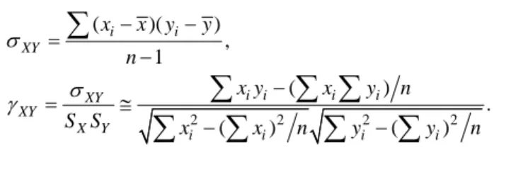
Three sets of counting data were used for comparison, with one being the system count and two being manual counts. The experiment analysis method proposed by J. Dahle and M. Kakar [4] was adopted along with Karl Pearson product-moment correla-tion. For the product-moment correlation formula, the sample covariance [15] must first be determined and this is defined by Eq. (22). The formula for the Pearson product-mo- ment correlation is then as Eq. (23). Here, γXY is the Pearson product-moment relation, σXY

Table 1. Codes for all experimental conditions.

Heating time Temperature 37°C Temperature 41°C Temperature 42.5°C

0.5h Tc1 Tc5 Tc9

1h Tc2 Tc6 Tc10 2h Tc3 Tc7 Tc11 4h Tc4 Tc8 Tc12

the specimen co-variance, SX the standard deviation for specimen X and SY the standard deviation for specimen Y. Every value xi corresponds to a value yi. n is the total number of X specimens, and by default, the total number of Y specimens as well.

( )( ) , 1 i i XY x x y y n σ = − − −

∑

∑

∑ ∑

∑

∑

∑

∑

3. RESULTS AND DISCUSSION

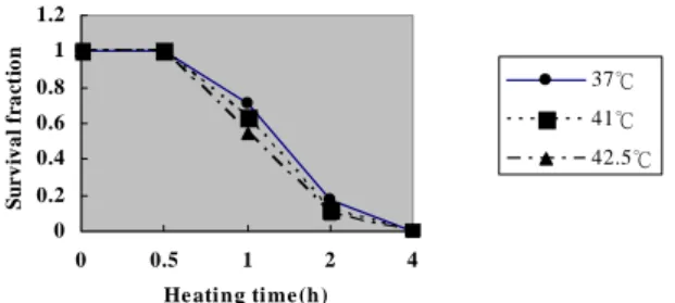
The results from the 12 experimental environments in this paper are compared using the methods proposed by J. Dahle [4] and N. Maximilian [2]. Table 2 shows the error rate between the three count types for each experimental environment and manual count 1, or the expert count. The Pearson product-moment correlation values and the data distribution are shown that rAM1 = 0.987, rAM2 = 0.983 and RM1M2 = 0.971. The experimental data in Table 2 were substituted into Eq. (26) using Excel software. The experimental data in Ta-ble 2 was also used with Excel software to produce Fig. 5.

Table 2. Comparison of the colonies number by manual and the system counting.

Experimental conditions Manual count 1 (M1) expert count (M2) System count (A1)* J. Dahle and M. Kakar [4] (N1) N. Maximilian and N. Ismat [2] (O1) error rate (A1-M1/M1) % error rate (N1-M1/M1) % error rate (O1-M1/M1) % Tc1 172 174 176 177 163 2.32% 2.9% − 5.23% Tc2 122 124 125 128 135 2.4% − 4.91% 10.65% Tc3 32 34 32 28 40 0 − 12.5% 25% Tc4 7 7 7 8 5 0 14.2% − 28.57% Tc5 126 128 127 120 133 0.79% − 4.76% 5.55% Tc6 79 85 82 73 81 3.79% − 7.59% 2.53% Tc7 15 16 16 18 17 6.67% 20% 13.33% Tc8 2 2 2 2 2 0 0 0 Tc9 88 89 92 97 93 3.4% 10.22% 5.68% Tc10 47 48 46 41 51 − 2.12% − 12.76% 8.51% Tc11 9 10 9 8 12 0 − 11.11% 33.33% Tc12 3 3 3 3 3 0 0 0

0 0.2 0.4 0.6 0.8 1 1.2 0 0.5 1 2 4 He ati ng ti me (h) S u r vi val f r ac ti on 37℃ 41℃ 42.5℃

Fig. 5. Comparison of survival fractions vs. heating time.

The γ values between system counts and manual counts 1 and 2 were all between 0.90 and 0.99, showing that system quantification is capable of replacing manual quantification. This implies that the image analysis system for automatically quantifying cancer cell col-ony can be applied to the Clonogenic Assay. The culture dish used for testing in Fig. 5 shows that when the standard 0.5h radiation treatment is used as the baseline, the length of radiotherapy time increased and the number of colonies decreased. The lower the tem-perature of the experimental environment, the faster the rate of decrease.

4. CONCLUSIONS

This paper proposes a fuzzy inference system (FIS)for determining whether or not a cancer cell colony contains more than 50 cells. The proposed system is also capable of counting how many cancer cell colonies with more than 50 cells are contained in a culture dish. The dish image’s 2-dimensional coordinates can be established using Hough trans-form’s line detection. Image differencing is then used to find the target image. Next, the color model features and surface area features are used in conjunction with the proposed fuzzy inference system (FIS) to determine if the cancer cell colony contains more than 50 cells. Experimental results show a very strong correlation between the quantities produced by the system and the quantities revealed by manual counting, with γ values that all exceed 0.9. Therefore, system counting can replace manual counting, reducing the manpower re-quired for Clonogenic Assays, accelerating the development of new drugs, and solving manpower problems in medicine. The fuzzy inference system (FIS) proposed in this sys-tem can also be used to identify problematic colonies. This boosts syssys-tem performance while avoiding missed counts or misjudgments that might influence test results.

REFERENCES

1. K. Kawada, T. Yonei, H. Ueoka, K. Kiura, M. Tabata, N. Takigawa, M. Harada, and M. Tanimoto, “Comparison of chemosensitivity tests: Clonogenic assay versus MTT as-say,” Acta Medica Okayama, Vol. 56, 2002, pp. 129-134.

2. N. Maximilian, N. Ismat, and B. Claus, “Counting colonies of clonogenic assay by using densitometric software,” Radiation Oncology, Vol. 2, 2007, pp. 2-4.

3. D. P. Berger, H. Henb, B. R. Winterhalter, and H. H. Fiebig, “The clonogenic assay with human tumor xenografts: evaluation, predictive value and application for drug

screening,” Annals of Oncology, Vol. 1, 1990, pp. 333-341.

4. J. Dahle, M. Kakar, H. B. Steen, and O. Kaalhus, “Automated counting of mammalian cell colonies by means of a flat bed scanner and image processing,” Cytometry Part A, Vol. 60, 2004, pp. 182-188.

5. J. Y. Rau and L. C. Chen, “Fast straight lines detection using Hough transform with principal axis analysis,” Aerial Survey and Telemetering Measurement Academy Pe-riodical, Vol. 8, 2003, pp. 15-34.

6. L. Rodrigues, D. B. Leandro, and L. G. Marcos, “A locally adaptive edge-preserving algorithm for image interpolation,” in Proceedings of IEEE International Conference on Computer Graphics and Image Processing, 2002, pp. 300-305.

7. R. O. Duda and R. E. Hart, “Use of the Hough transform to detect lines and curves in pictures,” Communications of the ACM, Vol. 15, 1972, pp. 11-15.

8. Y. L. Chan and J. K. Aggarwal, “Line correspondences from cooperating spatial and temporal grouping processes for a sequence of images,” Computer Vision and Image Understanding, Vol. 67, 1997, pp. 186-201.

9. H. Li, M. A. Lavin, and R. J. LeMaster, “Fast Hough transform: A hierarchical ap-proach,” Computer Vision, Graphics and Image Processing, Vol. 36, 1986, pp. 139- 161.

10. N. Kanopoulos, N. Yasanthavada, and R. Baker, “Design of an image edge detection filter using the Sobel operator,” IEEE Journal of Solid State Circuits, Vol. 23, 1988, pp. 358-67.

11. F. Lv, T. Zhao, and R. Nevatia, “Self-calibration of a camera from video of a walking human,” in Proceedings of International Conference on Pattern Recognition, Vol. 1, 2002, pp. 562-567.

12. R. C. Gonzalez and R. E. Woods, Digital Image Processing, Upper Saddle River, Prentice Hall, NJ, 2002.

13. http://www.ym.edu.tw/humn/.

14. C. T. Lin and C. S. G. Lee, Neural Fuzzy Systems: A Neuro-Fuzzy Synergism to Intel-ligent Systems, Upper Saddle River, Prentice Hall, NJ, 1996.

15. Z. Y. Zhan and S. P. Lai, The Fundamental Statistic Application with Excel, Publica-tion of NaPublica-tional Library, www.nou.edu.tw, 2005.

Sheng-Fuu Lin (林昇甫) was born in Taiwan, R.O.C., in 1954. He received the B.S. and M.S. degrees in Mathematics from National Taiwan Normal University in 1976 and 1979, respectively, the M.S. degree in Computer Science from the University of Maryland, College Park, in 1985, and the Ph.D. degree in Electrical Engineering from the University of Illinois, Champaign, in 1988. Since 1988, he has been on the faculty of the Department of Electrical and Control Engineering at National Chiao Tung University, Hsinchu, Tai-wan, where he is currently a Professor. His research interests include image processing, image recognition, fuzzy theory, automatic target recognition, and scheduling.

Hsien-Tse Chen (陳弦澤) was born in Taipei, Taiwan, R.O.C., in 1977. He received the B.S. degree in Department of Marine Engineering from National Taiwan Ocean Uni-versity, Keelung, Taiwan, R.O.C., in 1999 and the M.S. degree in Department of

Auto-matic Control Engineering from Feng Chia University, Taichung, Taiwan, R.O.C., in 2002. He is currently pursuing the Ph.D. degree in the Department of Electrical and Control En-gineering, the National Chiao Tung University, Hsinchu, Taiwan. His current research interests include image recognition, medicine image processing, machine vision.

Yi-Hsien Lin (林宜賢) was born in Taiwan, in 1973. He received the M.D. degree from the School of Medicine of National Yang Ming University, Taipei, Taiwan, in 1998. He received medical training at Cancer Center of Taipei Veterans General Hospital since 2000 and became a board-certified specialist in Radiotherapy in 2004. Now he is the attending physician of Division of Radiotherapy, Cheng Hisn Rehabilitation Medical Center, Taipei, Taiwan. He is also the Ph.D. candidate of Institute of Traditional Medicine, National Yang Ming University. His research interests include radiation physics and bi-ology, cancer bibi-ology, traditional medicine.