A two-point method for estimating wave reflection over a sloping beach

www.elsevier.com/locate/oceaneng

A two-point method for estimating wave

reflection over a sloping beach

H.-K. Chang

_{, T.-W. Hsu}

a_{Department of Civil Engineering, National Chiao Tung University, Hsinchu 300, Taiwan} b_{Department of Hydraulic and Ocean Engineering, National Cheng Kung University, Tainan 701,}

Taiwan

Received 26 May 2002; received in revised form 1 September 2002; accepted 30 September 2002

Abstract

This work presents a frequency-domain method for estimating incident and reflected waves when normally incident waves’ propagating over a sloping beach in a wave flume is con-sidered. Linear wave shoaling is applied to determine changes of the wave amplitude and phase due to variations of the bathymetry. The wave reflection coefficient is estimated using wave heights measured at two fixed wave gauges with a distance. The present model demon-strates a high capacity of estimating reflection and shoaling coefficients from synthetic wave-amplitude data. Sensitivity tests for the present model due to measurement errors of wave amplitudes and distance of two probes can more accurately predict the reflection coefficients. The measurement error of wave amplitude affects more significantly than measurement error of distance of two probes on calculating reflection coefficient of waves over a sloping bed.

2003 Elsevier Science Ltd. All rights reserved.

Keywords: Waves reflection; Frequency domain; Sloping bathymetry

1. Introduction

Wave reflection from natural beaches and man-made coastal structures influences the hydrodynamics and the sediment transport in front of the reflector. It is therefore important to understand the nature of the reflection coefficients accurately for engin-eering practice. The wave reflection of marine structures or their armored boundaries

∗ _{Corresponding author.}

E-mail address: [email protected] (H.-K. Chang).

0029-8018/03/$ - see front matter2003 Elsevier Science Ltd. All rights reserved. doi:10.1016/S0029-8018(03)00017-9

is usually tested to examine their performances by two- or three-dimensional physical models before such structures are constructed. In general the reflection coefficient of marine structures is one of important examination items. On the other hand, it is desirable to separate the wave train into the incident and reflected waves so that the reflection coefficient can be related to incident wave and structure properties in many studies. The marine structures in site are usually constructed on sloping natural beds. The sloping bed that can reflect the wave adds an additional reflection coefficient to the reflected wave from marine structures. Thus, the combined reflection coefficients include two parts. One part is due to the sloping bed and the other one is due to marine structures. The superposition of the incident and reflected waves on a sloping bed increases additional difficulty in estimating the reflection coefficient due to slop-ing effect.

This problem has been addressed for more than five decades. The conventional method of Healy (1952) used the maximum and minimum of the standing wave envelope to estimate the reflection coefficients of regular waves. This method is to slowly move a wave gauge in a wave flume in the direction of wave propagation.

Isaacson (1991)noted that using an array of fixed wave gauges to determine reflec-tion coefficients is preferred to using a moving single gauge.Hughes (1993)reviewed three commonly used methods using fixed wave gauges and the corresponding wave parameters listed as follows. (I) Two wave heights and one wave phase at two fixed wave gauges (Goda and Suzuki, 1976); (II) Three fixed wave gauges measuring three wave heights and two wave phases (Mansard and Funke, 1980); (III) Three fixed wave gauges measuring three wave heights (Isaacson, 1991). The first method is frequently used in two dimensional laboratory studies, and it offers a valuable tech-nique for examining wave reflections from coastal structures. Method II affords more conditions than unknowns, and needs a least-square method to fit the data. The third method avoids the need of measuring the phase shift between the wave gauges. All these methods are based on the frequency domain so that they can be applied to regular and irregular waves over horizontal bottom only.

Recently Frigaard and Brorsen (1995) applied two theoretical phase shifts and amplification to digital filters to efficiently separate reflected wave from wave field in real time. Hwang and Shieh (1994)added weighting factors to amplitudes of any two wave gauges and gave more accurate prediction to wave reflection from oblique incident wave to a structure.Baquerizo et al. (1997)presented a new method using root-mean-square wave height and set-up at three gauges to estimate the cross vari-ations of wave reflection for random waves over a sloping bottom. A different method of Guza and Bowen (1976) and of Tatavarti et al. (1988) uses collocated current and elevation/pressure sensors, where the current provides information on the slope of the sea surface from which waves’ propagating direction can be esti-mated. This method overcomes the variability in bathymetry, but the reflection coef-ficients obtained are increased by noise (Huntley et al., 1999). Huntley et al. (1999)

developed two methods of using collocated measurements of elevations and horizon-tal current to estimate frequency dependent reflection coefficients for irregular waves. Recently, Medina (2001) proposed a time-domain local approximation model in which linear, the second-order Stokes nonlinear components, and a simulated

annealing algorithm are considered to separate incident and reflected waves using several wave gauges.

The methods mentioned above are only available for the case of two-dimensional waves propagating over a horizontal bed and are presently used by several labora-tories for a wide range of applications. However, none of these methods strictly explain the reflection coefficient of propagating waves over a sloping beach. How-ever, errors in the reflection analysis on waves over a bed with arbitrary bathymetry are likely arisen, depending on the wave conditions and bottom slope.Baldock and Simminds (1999)modified Frigaard and Brorsen’s (1995) time series to account for normally incident linear waves propagating over seabed with arbitrary bathymetry. They found that the errors in estimated reflection coefficients are small for the case of high wave reflection, but become large for low wave reflection. They also noted that accounting for the bathymetry significantly reduces the errors in estimating the amplitudes of local incident and reflected waves. This implies that the effects of a sloping bottom on the amplitudes and phases of incident and reflected waves must be considered in the method for estimating reflection coefficient of waves over a sloping bed.

The purpose of this paper is to present a simple frequency-domain method for separating incident and reflected waves to account for normally incident linear waves propagating over a sloping bed with arbitrary 2-D bathymetry. Linear wave shoaling theory is used to determine changes of wave height and phase due to the variations of bathymetry. The reflection coefficient is estimated from two wave heights meas-ured at two fixed gauges with a distance. This method is applicable to laboratory conditions and also to field data for predominantly shore normal propagating waves when the incident wave at deep water is given. However, wave breaking is not considered in the present paper. The validity of the present model is proven using synthetic wave-amplitude data of waves propagating over a sloping bottom. The possible influence of measurement errors, for example, in wave height and the space between two wave gauges, on reflection of waves is discussed in a view of engineer-ing practice.

2. Theoretical formulation

The coordinate system for waves propagating over an arbitrary bathymetry is shown inFig. 1. Linear wave theory (designated as LWT) gives water surface elev-ation, h, at a spatial location x corresponding to the mean water depth h as

h(x,t)⫽ aicos(

冕

冕

where t = the time, s = the angular frequency, a = the wave amplitude, k = the wave number,⑀=the phase shift, and the subscripts i and r denote the incident and reflected components, respectively. As shown in Fig. 1 two probes are located at

Fig. 1. Definition of coordinate system for waves propagating over a sloping bed.

xfis symbolized by xm. The origin of this coordinate is on the shoreline and positive

x axis points seawards.

Using trigonometric identities and rearranging Eq. (1) leads to the wave amplitude at any location |h|⫽ ai

冋

冕

册

ai⫽ a0ks (3)

where a0is the wave amplitude at deep water, and ksis the shoaling coefficient that can be calculated by the following formula based on LWT.

ks⫽

冉

kh

cosh2_kh

冊

⫺1₂

(4) The spatial phase function at the location xfis expressed as

冕

冕

冕

The first term on the right hand side represents the accumulated spatial phase from the shoreline to the central location xm. The second term describes the phase shift due to the distance from xmto xf. Because the wave number varies with water depth in the x direction, the integration of Eq. (5) cannot be analytically integrated. Apply-ing mean value theory to integrate of the second term yields

冕

冕

冉

冊

|

km = k(xm) and dk / dx at the location xm. The derivative of k with respect to x can be obtained using linear dispersion relation in the association with the chain rule.

dk dx⫽ dk d(kh) d(kh) dx ⫽ ⫺k2_tanb kh⫹1 2sinh(2kh) (7)

where tanb is the local average bottom slope. For a horizontal bottom, the derivative

dk / dx is equal to zero because tanb=0, indicating that the wave over a horizontal bottom keeps a constant wave number in the direction of propagation. In this case, the phase shift depends only on the distance of two probes. In deep water kh → ⬁, dk/dx approaches zero because the denominator of Eq. (7) becomes infinite for a finite value of k. This means that the depth variation in deep water hardly affects the wave number. However, in the shallow water zone, dk /dx approaches ⫺ k tan b / 2h owing to the approximation, sinh 2kh → 2kh. This shows that the depth of shallow water significantly effects on the wave number. Substitution of Eqs. (3)–(7) into Eq. (2) leads to the following expressions for the wave amplitudes at locations

xb and xf, respectively |h|b⫽ a0ksb[1⫹ R2 ⫹ 2Rcos(q⫺a ⫹ ⌬a)] 1 2 ₍₈₎ |h|f⫽ a0ksf[1⫹ R 2⫹ 2Rcos(q ⫹ a ⫹ ⌬a)] 1 2 ₍₉₎ where q⫽ 2

冕

Eq. (10a) represents an unknown phase to be determined. Eq. (10b) illustrates one spatial phase shift by the distance between two probes. Eq. (10c) specifies the other spatial phase shift affected by variations of the wave number due to changes of water depth and bottom slope. When the wave amplitudes of two probes are measured for the case of giving incident wave amplitude a0and wave period T in prior, the

reflec-tion coefficient and spatial phase shift can be obtained from Eqs. (8) and (9). It is convenient to use two new variables to represent the ratio of the wave amplitude to the shoaling coefficient at location xb and xf, respectively.

B⫽|hb| ksb (11) F⫽|hf| ksf (12)

The reflection coefficient is solved from Eqs. (8)– (10) and (12) as R⫽ F 2⫺B2 4a2 0sin(q⫹ ⌬a)sina (13) The denominator of Eq. (13) becomes zero if the value of sin(θ +⌬a) or sin a equals zero so that the reflection coefficient turns out to be infinite. The constraint condition of sin a =0 means that a = np. An alternative expression of Eq. (10b) for this case is

⌬x ⫽nLm

2 , n ⫽ 1,2,3… (14)

where Lm is the wavelength at the location xm. Eq. (14) indicates that the reflection coefficient becomes infinite if the distance between two probes is an integer multiple of half the wavelength at the central location. If ⌬x = (nLm) / 2 the present model fails to estimate reflection coefficient. Goda and Suzuki (1976)also found this con-straint and recommended the distance to be confined by 0.05⬍ ⌬x/L ⬍ 0.45. The other case of sin(q + ⌬a)= 0 indicates that (q + ⌬a)= np from the definition of sine function. This result points out that the values of cos(np – a) and cos(np + a) in Eqs. (8) and (9) are the same. Eqs. (8) and (9) are identical to one equation so that the reflection coefficient becomes irresoluble. Inserting Eq. (13) into Eq. (9), we obtain a quadratic equation for q that is expressed as

q⫽ tan⫺1

冉

冑

冊

In Eq. (15) the sign of positive or negative to be taken depends on the limiting condition of 0 ⱕ R ⱕ 1. The amplitude of incident wave and reflected wave at arbitrary water depth can be estimated by the following equations, respectively:

ai⫽ |hf| [1⫹ R2⫹ 2Rcos(q ⫹ a ⫹ ⌬a)]1 2 (17) and ar⫽ aiR (18)

If a hydraulic model test in a wave flume was carried out to estimate reflection coefficient of regular waves from a structure over a sloping bed, the reflection coef-ficient can be determined by the present method as the following steps. Two wave gauges with a distance of ⌬x are set in front of the structure to measure the wave

amplitude at each probe. The average bottom slope is estimated by tan b = (hf –

hb) /⌬x. The shoaling coefficients ksband ksfcan be obtained by Eq. (4) for a given wave period T and water depths at both two probes. The values of B and F are calculated using Eqs. (8) and (9) with observed wave amplitudes at xm and xf and computed shoaling coefficients. The spatial phase shiftsa and⌬a are then calculated by Eqs. (10b and c) to obtain q by Eq. (15). Finally the reflection coefficient is determined by Eq. (13). Thus the incident and reflected waves can be separated by Eqs. (3) and (8).

The time-domain method for separating wave reflection from the combined waves is a real-time tool to detect data quality analysis including the signal quality and input condition. It has the benefit of offering an in-time response. When real-time information cannot be obtained, a frequency-domain method is developed on the basis of regular waves. When measured data of random waves are divided into many components, each component can be considered to be a regular wave with its corre-sponding frequency. For the case of random waves, the measured water surface elev-ation can be transformed into a wave energy spectrum using Fast Fourier Transform-ation (FFT). The wave amplitude of a given spectrum is evaluated by a(f) =(4S(f)

df)1 / 2_{, where S(f) is the wave energy spectrum, of the frequency interval. The}

reflec-tion coefficient is estimated by Eq. (13) if the amplitude is obtained from the observed spectrums of two wave probes. We thus conclude that the present method can provide a valuable tool to calculate wave reflection coefficient of random waves.

3. Synthetic waves propagating over a sloping bottom

In order to examine the validity of the present method for wave reflection over a sloping bottom, we choose a linear wave theory ofGuza and Bowen (1976)to calcu-late the wave amplitudes in the waves’ propagating direction. Guza and Bowen (1976) derived a general solution of the velocity potential for waves propagating over a sloping bed in which they addressed the matching theory to both the deep-water limit and shallow deep-water limit. The total velocity potential is written as

f⫽ fs⫹ fd⫺flim (19)

where f is the total velocity potential, fs, fd and flim are the velocity potentials in

the shallow water, deep water, and intermediate water, respectively. We rearrange these velocity potentials originally given by Guza and Bowen (1976) as follows

fs⫽

a0g

s p

2tanb{J0(c)cosst⫺Y0(c)sinst ⫹ R[J0(c)cos(st⫺q) (20) ⫹ Y0(c)sin(st⫺q0)]} fd⫽ a0ksg s coshk(z⫹ h) coshkh [cos

冉冕

冊

冉冕

冊

flim⫽ a0g s

冑

冋

冉

冊

冉

冊册

in which χ2 = _4s2_{x / (g tanb), f}= _{the phase shift function, q}

0 =the phase shift of

incident waves, J0and Y0are Bessel functions for the first and second kind,

respect-ively. The dimensionless relative water depth is expressed as

h_∗⫽s

2_h

g ⫽

s2_xtanb

g (23)

The water surface elevations valid for these three depth regions are obtained through linear dynamic free surface boundary condition, i.e., h = ⫺[∂f /∂t]z=0/ g.

The expression of water surface elevation is written after some algebraic manipu-lations

h(x,t)⫽ Ccosst ⫹ Ssinst (24)

with

C⫽ ( p

2tanb)a0[Y0(c)⫺RJ0(c)sinq0⫺RY0(c)cosq0]⫹ a0ks

冋

冕

冕

册

冑

冋

册

2tanb)a0[J0(c)⫹ RJ0(c)cosq0⫺RY0(c)sinq0]⫹ a0ks

冋

冕

冕

册

冑

冋

册

Both amplitudes C and S can be determined when the wave conditions, a0, T,

bottom slope tanb, and phase functions f and q0 are given. The variation of wave

amplitude at different locations is thus obtained by √C2_{+ S}2_{. Typical values of a} 0

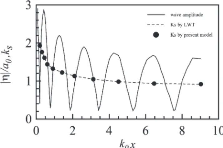
=1 m, T =10 s, tan b= 1 / 40 and R =0.2 in practical coastal area are chosen to calculate wave amplitudes by Eq. (25). Fig. 2 shows the computed relative wave amplitudes in the direction of propagation. It is obviously seen that the partial stand-ing waves are formed and the relative wave amplitudes vary as an envelope in the direction of propagation. Larger variations of relative wave amplitudes near the

Fig. 2. Calculated wave amplitude and shoaling coefficient. (T=10 s, tanb=1 / 40, R=0.2).

shoreline than farther from the shoreline result from wave shoaling and wave reflec-tion due to depth variareflec-tion. The good agreement between the predicted shoaling coefficient and the theoretical one substantiates the present method as valid for separ-ating reflected and incident waves over a sloping bed.

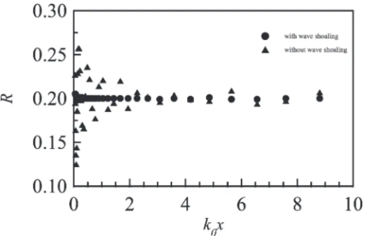
Fig. 3shows the estimated reflection coefficient considering or neglecting wave shoaling under the same conditions asFig. 2. Solid circles and open circles, respect-ively, represent the computed reflection coefficient with and without wave shoaling effects. Neglecting wave shoaling in the computation means dropping off the shoa-ling coefficients from Eqs. (11) and (12). In these computations the estimated reflec-tion coefficients using the present method approach 0.2 that is the specified reflecreflec-tion coefficient in the synthetic waves. This result demonstrates that the present method has a more accurate prediction to estimate reflection of the coefficient of waves over

Fig. 3. Computed reflection coefficient using the present method with or without considering wave shoa-ling. (T=10 s, tanb=1 / 40, R=0.2)

a sloping bed than the method without considering the shoaling effect.Fig. 3shows a large disparity of estimated reflection coefficient from 0.2 near the shoreline and a small deviation away the region from the shoreline when the effect of wave shoa-ling is omitted. On the contrary, the present method considering wave shoashoa-ling almost keeps an estimated reflection coefficient of 0.2 for all relative depth ranges. Because wave shoaling in the shallow water becomes important wave shoaling can-not be neglected in the calculation of wave reflection over a sloping bed.

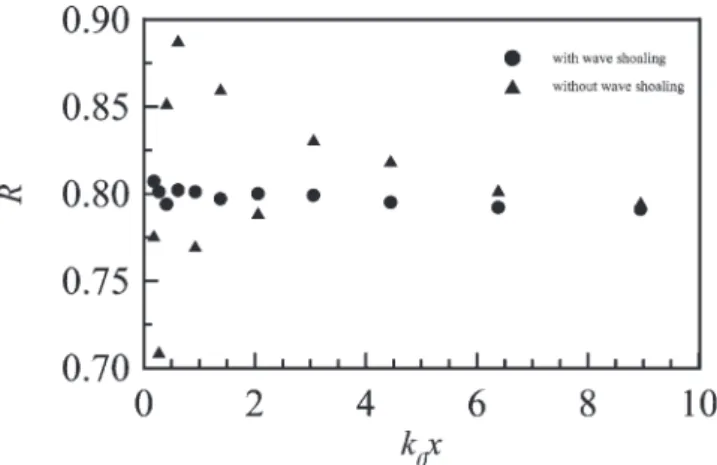
The input parameters of T = 10 s, R = 0.8 and tan b = 1 / 10 are specified to another case. This case has a high reflection coefficient due to a steep slope bottom. The combined wave amplitudes and shoaling coefficients are plotted in Fig. 4. A comparison betweenFig. 2 andFig. 4 explains thatFig. 4 has a larger variation of water amplitudes of partial standing waves thanFig. 2because of the steeply sloping bottom. The present model also presents a good agreement with the shoaling coef-ficient with LWT over the whole depth ranges.

Fig. 5 shows the estimated reflection coefficient using the present method with and without considering wave shoaling. When wave shoaling is included, the com-puted wave reflection deviates from the specified value of 0.8 only by a relative error 2.5% for the region of the shoreline to k0x= 4.5 at which the relative water

depth h / L is about 1/8.7. Comparing with Fig. 2 the relative error of estimated reflection coefficient exceeding 2.5% occurs in the region from the shoreline to the relative depth h / L⬇ 1/30. Estimated reflection coefficient of waves on a steep slope bottom has a larger disparity than that on a mild slope bottom at the same relative water depth. We thus conclude that the bottom slope is also an important factor in estimating wave reflection over a sloping bed.

4. Sensitivity tests for measurement errors

In practical wave measurements made in the laboratory or the field, some tolerant measurement errors maybe happen. These possible errors cause the estimated wave reflection from the actual reflection.

Fig. 5. Computed reflection coefficients by the present method with or without considering wave shoa-ling. (T=10 s, tanb=1 / 10, R=0.8).

Fig. 6 shows the predicted wave reflections calculated from Eq. (13) when observed wave amplitudes at two probes are overestimated or underestimated by an error of 3% for a mild slope bottom. Solid triangles and squares, respectively, present the predicted reflection for both cases. We note that the estimated reflection coef-ficient deviates from the specified value by an error of 0.05 for all water depth ranges.

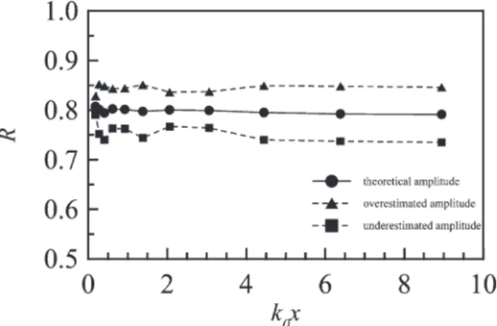
Fig. 7 shows the computed wave reflections under the same input wave conditions asFig. 6but for a steep slope bottom. Overestimation of the incident wave amplitude induces an over-predicted reflection coefficient. Contrarily underestimation of the incident wave amplitude produces an under-predicted reflection coefficient. The esti-mated reflection coefficients only vary by errors less than 5% over the whole water depth regions for both cases of overestimated and underestimated incident wave

Fig. 6. Computed reflection coefficients using overestimated or underestimated T=10 s, tanβ =1 /40, R=0.2

Fig. 7. Computed reflection coefficients using overestimated or underestimated T=10 s, tanβ =1 /10, R=0.8

amplitude. This sensitivity test indicates that the estimated wave reflection has a nearly equivalent relative error to the measurement error oft wave amplitude of two probes.

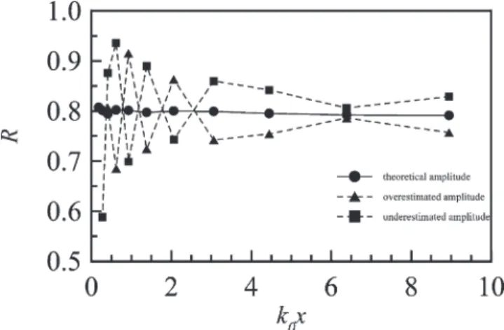
Fig. 8 shows the estimated reflection coefficients with a relative error of wave amplitudes at two probes by 3% for a mild slope bottom. Solid triangles and squares, respectively, illustrate the estimated reflection coefficients for the conditions of overestimation and underestimation of incident wave amplitudes. The relative error of the predicted reflection coefficient is over 25% for k0x⬍ 2.0. It is shown in Fig. 8 that a larger deviation of the estimated reflection coefficient from the specified value due to the overestimated or underestimated amplitudes of two probes occurs

Fig. 8. Computed reflection coefficients using overestimated or underestimated amplitudes of two probes. (T=10 s, tanb=1 / 40, R=0.2).

Fig. 9. Computed reflection coefficients using overestimated or underestimated amplitudes of two probes. (T=10 s, tanb=1 / 10, R=0.8).

near the shoreline rather than that at offshore.Fig. 9shows the results of sensitivity test for the case of a steep bed. The estimated wave reflection also has a large deviation from the specified value for k0x⬍ 2.0. The variations of estimated wave

reflections due to measurement errors of wave amplitudes display a similar tendency for both mild and steep bottoms.

Fig. 10 presents a sensitivity examination on estimating reflection coefficient resulting from measurement error of distance ⌬x by an error of ± 3% for a mild slope bed. It is shown that the relative error of estimated reflection coefficient differs

Fig. 10. Computed reflection coefficients using overestimated or underestimated distance of two probes. (T=10 s, tanb=1 / 40, R=0.2).

Fig. 11. Computed reflection coefficients using overestimated or underestimated distance of two probes. (T=10 s, tanb=1 / 10, R=0.8).

from the specified value by only about ±3% for all water depth regions. Fig. 11

illustrates the predicted reflection coefficient under the same condition as Fig. 10

but for the steep slope bed. It is also found that a slight deviation of estimated reflection coefficient varies from the specified value for all water depth regions. This result indicates that the measurement error of the distance of two probes hardly affects on estimating on the reflection coefficient of waves over a sloping bed.

5. Conclusion

A frequency-domain method for separating incident and reflected waves is pro-posed in this paper to account for normal incident waves propagating over a sloping beach. The wave reflection coefficient is estimated by using wave heights at two fixed wave gauges with a distance. Brief comparisons between the predicted reflec-tion coefficient and shoaling coefficient and the given values in synthetic wave data are made to show the present model having a high capacity of estimating reflected wave and incident wave over a sloping bed. The water depth in the shallow water and steep slope strongly affect estimation of wave reflection over a sloping bed. A sensitivity test demonstrated the present method’s validity for predicting the wave reflection coefficient for possible measurement errors on wave amplitudes and the distance of two probes. Two probes’ correctly measuring the wave amplitudes is more important than the distance in estimating the reflection coefficient.

Acknowledgements

The authors would like to thank the National Science Council of the Republic of China financially supporting this research under contract number of NSC 89-2611-E006-033.

References

Baldock, T.E., Simminds, J.M., 1999. Separation of incident and reflected waves over sloping bathymetry. Coastal Engineering 38, 167–176.

Baquerizo, A., Lasoda, M.A., Smith, J.M., Kobayashi, N., 1997. Cross-shore variation of wave reflection from beaches. J. Waterway, Port, Coastal Ocean Engineering 123, 274–279.

Frigaard, P., Brorsen, M., 1995. A time domain method for separating incident and reflected irregular waves. Coastal Engineering 24, 205–215.

Goda, Y., Suzuki, Y., 1976. Estimation of incident and reflected waves in random waves. Proc. Int. 15th Conf. on Coastal Engineering, ASCE, New York, pp. 828-845.

Guza, R.T, Bowen, A.J., 1976. Resonant interactions for waves breaking on a beach. Proc. Int. 15th Conf. on Coastal Engineering, ASCE, New York, pp. 560-579.

Healy, J.J., 1952. Wave damping effect of beaches. Proc. Int. Hydraulics Convention, 213-220. Hughes, S.A., 1993. Laboratory wave reflection analysis using co-located gages. Coastal Engineering 20,

223–247.

Huntley, D.A., Simmonds, D., Tatavarti, R., 1999. Use of collocated sensors to measure coastal wave reflection. J. Waterway, Port, Coastal Ocean Engineering 125 (1), 46–52.

Hwang, J.S., Shieh, J.C., 1994. Study on methods to separate obliquely incident and reflected waves. Proc. 16th Conf. Ocean Engineering, Kaohsiung, Taiwan, pp. B-268-287 (in Chinese).

Isaacson, M., 1991. Measurement of regular wave reflection. J. Waterway, Port, Coastal and Ocean Engin-eering 117 (6), 553–569.

Mansard, E.P.D., Funke, E.R., 1980. The measurement of incident and reflected spectra using a least squares method. Proc. Int. 17th Conf. on Coastal Engineering, ASCE, pp. 154-172.

Medina, J.R., 2001. Estimation of incident and reflected waves using simulated annealing. J. Waterway, Port, Coastal Ocean Engineering 127 (4), 213–221.

Tatavarti, R.V., Huntley, D.A., Bowen, A.J., 1988. Incoming and outgoing wave interactions on beaches. Proc. Int. 21st Conf. on Coastal Engineering, ASCE, pp. 136-150.