下一世代無線行動接取技術---總計畫：下一世代無線行動接取技術(I)

行政院國家科學委員會專題研究計畫 期中進度報告

總計畫:下一世代無線行動接取技術(1/2)

計畫類別： 整合型計畫 計畫編號： NSC94-2213-E-009-055- 執行期間： 94 年 08 月 01 日至 95 年 07 月 31 日 執行單位： 國立交通大學電信工程學系(所) 計畫主持人： 蘇育德 計畫參與人員： 黃汀華、劉人仰、廖明&#22531；、陳青煒 報告類型： 精簡報告 處理方式： 本計畫可公開查詢

中 華 民 國 95 年 5 月 30 日

行政院國家科學委員會專題研究計畫成果報告

下一世代無線行動接取技術-總計畫

Next Generation Mobile Radio Access Technologies (1/2)

計畫編號：NSC 93-2218-E-009-015 執行期限：94 年 8 月 1 日至 95 年 7 月 31 日 主持人： 蘇育德 國立交通大學電信工程學系 計畫參與人員：黃汀華、劉人仰、廖明堃、陳青煒 中文摘要 在第三代的通訊系統技術已進入商業 化的程序之後，無論是學界或工業界都已 開始在討論著下一代的通訊系統 (Beyond Third Generation, B3G)的可能架構與技 術。新一代的通訊系統(B3G)預期將提供 更全面性的服務，包括高速的資料傳輸、 多媒體服務及數據行動通訊，使無線通訊 的產業更加蓬勃。 雖然下一代的通訊系統的完整架構仍 在討論，但是我們可以確定的是B3G 無線 通訊系統的設計核心仍是在新的傳輸介面 (Air Interface)，即無線接取技術(Wireless Access Technology)之確立。 本總計畫含括三個子計劃，計劃名稱 分別為： (1) 下一世代無線行動接取技術 - 子計 劃一:多通道多速率展頻技術。 (2) 下一世代無線行動接取技術 - 子計 畫三:時空信號處理及多用戶檢測。 (3) 下一世代無線行動接取技術 - 子計 劃四:同步、通道估計與內接收機設計。 各個子計劃所發展的成果將在本報告 中以獨立章節做一重點性的說明，並輔以 軟體模擬成果以提供完整的系統性能評估 之用。本報告為二年期計劃中第一年相關 研究成果的總體精簡報告。 關鍵詞：無線通訊，行動無線接取技術， B3G。 Abstract

As the 3G systems have been deployed and commercialized, research institutes, major equipment providers as well as op-erators from all over the world had joined forces to look into future generations (be-yond the third generation, B3G) of wireless communications, creating the Wireless World Research Forum (WWRF).

It is expected that the air interface will be playing the central role of the B3G wire-less network. In this report, we propose a new broadband wireless mobile access ar-chitecture that is suitable for high-speed multimedia wireless transmission, predict its overall performance, and validate its feasi-bility. We produce simulation programs so that future users can emulate the perform-ance of our joint design. This joint effort consists of tree sub-projects, namely,

1. Multi-channel multi-rate spreading se-quences technologies.

3. Space-time signals processing and multi-user detection.

4. Synchronization, channel estimation and inner receiver design.

It is clear that each sub-project studies a vital part of a broadband wireless mobile

transmission system and all of them are closely coupled. For detailed description of each sub-project please refer to the sub-project reports.

Keywords: Wireless Communications,

Mobile Radio Access Technologies, B3G.

1. Introduction 下一代新的無線接取技術到底為 何，是繼續發展、改善 3G 的 CDMA 技術或需要新的接取技術，雖然以 歐、日大廠的研發趨勢與成果來判斷 後者的可能性較高，但現在尚無法確 定。就目前的資料來看，基本的傳輸 要求至少包括了： (1). 低速環境傳輸率 > 155 Mbps (2). 低速環境傳輸率 > 2 Mbps (3). 系統容量 > 10 倍 3G 容量 要達到這個目標當然得要改善3G 的 傳輸技術。本計畫所從事研究之接取技 術，係為目前無線寬頻通訊產、學業中積 極發展，頗具潛力的研究課題，也是未來 B3G 無線通訊系統運用所需建立的關鍵 技術。我們研發的成果，累積的技術能量 可提供業界諮詢，所培訓人員更可給予國 內通訊產業運用。除此之外，本計畫所研 究具備高效率、高彈性、高適應性的系統 架構，可供完整的系統性能模擬、評估之 用。 我們這個計畫分為三個子計畫，將分別就 這些發展中技術做深入的研究。三個子計 畫的名稱與主持人為： 一、 下一世代無線行動接取技術：多通 道多速率展頻技術（中興大學 楊谷 章教授） 二、 下一世代無線行動接取技術：時空 信號處理及多用戶檢測（中興大學 翁芳標助理教授） 三、 下一世代無線行動接取技術: 同 步、通道估計與內接收機設計（交通 大學 蘇育德教授） 以上三個子計畫在整個傳輸介面所探討 的部分及互相之整合程度請參見各子計 畫計畫書。綜合言之，各子計畫負責傳輸 介面的一特定環節，互補性與相關性至為 明顯，缺一不可。基本上，我們是以可調 式多天線、多傳輸率的OFDM/CDMA 系 統為基礎架構。我們的研究成果除了可運 用於 B3G 的行動通訊外，也旁及無線區 域網路如 IEEE 802.11a、g，個人區域網 路(Wireless Personal Area Network, WPAN) 及廣域網路如IEEE 802.16 等之應用。 在下列章節中，我們將就各子計劃去年 的成果做一重點性說明。 2. 下一世代無線行動接取技術-子計劃一: 多通道多速率展頻技術 2.1 Introduction

In the MC/DS-CDMA systems, the system performance gets worse as the mul-tiple-access interference (MAI) increases. Therefore, a new class of two dimensional orthogonal variable spreading factor (2-D OVSF) codes [2] was proposed to eliminate the MAI by the mutual orthogonality be-tween different users in the previous project. However, to maintain the code’s orthogonal-ity, the code cardinality of 2-D OVSF codes is restricted. Therefore, in order to support more subscribers and simultaneous users than the existing system using 2-D OVSF codes, a new 2-D non-orthogonal code, so-called frequency-hopping time-spreading codes are proposed in this project.

The new 2-D non-orthogonal codes which use Walsh codes and modified m-sequences for frequency-hopping, and Barker codes for time-spreading are pro-posed to increase the number of subscribers by utilizing two coding dimensions

simulta-neously. As a result, the overall code cardi-nality becomes a product of a quadratic function of the cardinality of the bipolar codes used for frequency hopping and a lin-ear function of the cardinality of the bipolar codes used for time-spreading. Therefore, the overall code cardinality is improved substantially.

2.2 Constructions of the 2D

Non-Orthogonal Codes

The 2-D frequency-hopping time-spreading codes (2-D FT codes) are obtained by the permutation of these multi-carrier codeword algebraically onto the time slots of another code chosen for time spreading. The algebraic permutation is controlled by prime sequences over Galois field of a prime number [3] in order to keep the cross-correlation functions of the result-ing 2-D FT codes as low as possible. The best candidate that can serve as the time spreading bipolar code in our 2-D FT cod-ing scheme is the family of Barker se-quences [4]. The reason for choosing the Barker sequences as our time-spreading bi-polar codes is because the maximum auto-correlation sidelobe of the barker sequence no more than one. The cross-correlation property is not that important because there exists only one Barker sequence that is used as the time spreading bipolar codeword for a given length. In other words, any bipolar codes with good autocorrelation property can also be used for time spreading in our 2-D FT codes.

The construction of the synchronized prime sequences begins withGF( )p of a

prime number p,S_{i l,} =(s_{i l, ,0},s_{i l, ,1},..., s_{i l p, , -1}),

such that si l j_{, ,} = ⊗ ⊕ , where i, j, and l (i j) l are all in GF( )p , “⊗” denotes a modulo-p

multiplication, and “⊕” denotes a modulo-p addition. As a result, p2 _distinct

synchro-nized prime sequences of length p are ob-tained. These p2 _{sequences can be}

parti-tioned in p groups of p sequences each. The first sequence in each group is the original

prime sequence, which generates other p-1 sequences in the group. The synchronized prime sequences have two correlation prop-erties [3]: 1) the cross-correlation function is at most one for any two prime sequences originated from different groups; 2) the cross-correlation function only occurs at the auto- correlation peak position but the func-tion can be as high as the autocorrelafunc-tion peak for any two prime sequences originated from the same group.

To generate the 2-D FT code matrices, we are going to permute the multi-carrier bipolar codewords into the time slot of the time-spreading bipolar codeword in accor-dance to the prime sequences over a Galois field GF( )p for a prime p. Each sequence

is used as a seed for generating a group of 2-D FT code matrices. The number of ma-trices in each group is determined by the number of available multi-carrier bipolar codewords (i.e., Φ ). The time-spreading _λ bipolar codeword has the length n=p. By permuting these Φ multi-carrier bipolar _λ codewords onto the n time slots of the time-spreading bipolar codeword in accor-dance to the patterns of the prime sequences, this gives Φgroup = groups of p Φ 2-D λ FT code matrices each and, thus,

2 p group FTC =Φ Φ = Φ _λ 2-D FT code matri-ces in total.

The performance of 2-D FT codes will be better by selecting some special code ma-trices from our 2-D FT codes. It means there is no interference when the number of si-multaneous users is less then p. Therefore, using the group property of the synchronous prime sequences, we can choose the group0 of matrices when the number of users is less than or equal to p; otherwise, we need to use multiple groups.

2.3 Performance Analysis

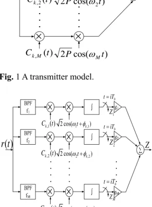
The average performance of the 2-D FT codes is analyzed and compared with that of 2-D OVSF codes and 2-D random codes in this section. The transmitter of the kth user

is shown in Fig. 1, wherek∈

{

1 K,2, ,K

}

and

K is the number of simultaneous users. We

separate the total bandwidth into M or-thogonal frequency bands of equal width. The binary data bit stream of the user k, bk(t),

is multiplied by the code sequence Ck,m of

length N and is transmitted by the mth fre-quency carrier wm, where m∈

{

1 K,2, ,M

}

and Ck,m represents the mth row of the

dis-tinct 2-D code matrix of size M×N desig-nated to user k, and M is the length of Walsh code.

The receiver of the kth user is shown in Fig. 2. By summing up all the MC/DS- CDMA signals at the receiver, the received signal is given by , , 1 1 , ( ) 2 ( ) ( ) cos( ) ( ), (1) K M k m k k k m k k m m k m r t P b t C t t n t α τ τ ω θ = = = − − ⋅ + +

∑∑

where n(t) is AWGN with a double-sided power spectrum density (PSD) of η₀ 2,

k

τ is the transmitted delay of user k, m

k ,

α and θ_{k ,m} are the amplitude and phase for user k in the mth channel, respectively. The MC/DS-CDMA signals detected at a receiver are first frequency-filtered into M diversity branches in accordance to the sig-nals’ carriers. The M filtered and despreaded signals Zk,m (form∈

{

1 K,2, ,M

}

), from a

de-cision sample (per bit period) are then com-bined by a linear combiner, such that

, 1

M k m m

Z =

∑

₌ Z . In this project, the

assump-tions of perfect carrier, bit, chip synchroni-zation and phase detections [1] are consid-ered. The filtered, despreaded and sampled output Z at the receiver is given by

(2) , η + + =S I Z

where S is the desired output of users, I is the despreaded interference term caused by other simultaneous users, and η is the fil-tered and despreaded AWGN term with a double sided PSD ofη0 2.

Assume that the MAI from other si-multaneous users and the noise after de-spreading at the receiver are zero-mean Gaussian independent random variables.

Then the mean of Z is given by

1, 1 [ ] (3) M b m m E Z PT α = = ±

∑

and the variances of Z is given by

[ ] [ ] [ ], (4)

VAR Z =VARη +VAR I

where VAR[ ]η =MTbη0 2. Therefore, the

signal-to-noise ratio (SNR) can be calculated and represented as [5], [6] 2_{[ ]} 2_{[ ]} . (5) [ ] [ ] [ ] E Z E Z SNR

VAR Z VAR I VARη

= =

+

In an AWGN channel, we can evaluate the error probability, Pe based on Gaussian

approximation, which is given by

( ), (6) e P =Q SNR where _{( )}

( )

₂ 1/ 2 _exp( 2 ₂₎ x Q x = π −

∫

∞ −z dz is

the Q-function.. In a Rayleigh fading chan-nel, the average bit error probability Pe is

given by [4] 0 ( ( )) ( ) , (7) e u P =

∫

∞Q SNR u ⋅ f u du where 2 2 2 2 ( ) u u u f u e σ σ −

= is the Rayleigh dis-tribution. Similarly, in a Rician fading channel, ( )f uu in (7) can be represented as

2 2 2 2 0 2 2 ( ) , (8) u v u u uv f u e σ I σ σ + − _{⎛ ⎞} = _{⎜ ⎟} ⎝ ⎠ where ₀

( )

1/ 2 2 0 ( ) 2 exp( cos ) I x = π −

∫

π x θ θd is

the modified zero-order Bessel function of the first kind [4], the Rice parameter is de-fined as 2 2

2 1

v + σ = and R≡v2 2σ2.

We apply Gaussian approximation to calculate the variances of MAI of the 2-D FT codes. As discussed in Section 2.2, the 2-D FT codes support at most 2

p

FTC = Φ

matrices. Using the group property of the synchronous prime sequences, we can choose the group 0 of matrices when the number of users is less than or equal to p; otherwise, we need to use multiple groups. Thus, the average variance of the

cross-correlation functions of the 2-D FT codes is generally given by

2g 2g p, 2g jp, , (9)

p K p

K K

σ =⎛_⎜ ×σ + − ×σ ⎞_⎟

⎝ ⎠

where2≤ j≤ p is the number of groups in

use. σ2g, p denotes the variance of the

cross-correlation functions in group 0 when ,

p

FTC =

Φ such that

σ2g p, =0. (10)

Such condition occurs only in the desired user and interferers are using the synchro-nized prime sequences from the group 0.

2 , jp

g

σ denotes the variance of the cross-correlation functions when Φ_FTC > p, such that [7]

(

)

(

)

(

)

2 2 ₁ , 2 2 2 1 1 1 1 1 , (11) 1 1 p g jp p t jp p j jp jp p p j j jp jp σ σ σ σ ⎡ − ⎤ = × ⎢ ⎥ − ⎢ ⎥ ⎣ ⎦ ⎡ − − ⎤ − + ×_⎢ + _⎥ − − ⎢ ⎥ ⎣ ⎦

where the first and second terms in (11) re-late to the variances of the cross-correlation functions of the desired multicarrier code-word originated from group 0 and group i (fori∈ p

[

1, −1

]

), respectively.σ is 2_p1

the variance of the cross-correlation func-tions created when the desired user and interferers are using the synchronized prime sequences from different groups. Thus, we have 2

(

1

)

. 1= K − p σ 2 1 t

σ is the variance of the cross-correlation functions created when the desired user and interferers are using the synchronized prime sequences from the same group. We then have 2

(

1

)

.

1 K N t = − σ

(

1

)

2 2 = K− p σ is derived similar to 2. 1 p σ The 2-D FT codes have the zero cross-correlation property, and thus, zero error probability. For supporting greater car-dinality, we can always select more than group 0 of synchronized prime sequences and the variance in (11) gets worse as more groups are used (i.e., j increases). In other words, we should choose the group 0 of

ma-trices when the number of users is less than or equal to p. For the number of users be-tween p+1 and 2

p

FTC =

Φ , we need to use multiple groups. For the case of the maxi-mum cardinality of 2

p

FTC =

Φ , the average variance [i.e., j=p in (11)] becomes

(

)

(

)

(

)

2 2 2 1 , ₂ 2 2 2 2 1 2 2 1 1 1 1 . (12) 1 1 p g jp p t p p p p p p p p p p p σ σ σ σ ⎡ ₋ ⎤ ⎢ ⎥ = × − ⎢ ⎥ ⎣ ⎦ ⎡ _{− −} ⎤ − _{⎢ ⎥} + × + − − ⎢ ⎥ ⎣ ⎦

The variances of MAI of the 2-D FT codes, 2-D OVSF codes and 2-D random codes under the different channels are summarized in Table I.

2.4 Numerical Analysis

Figs. 3 and 4 show error probabilities versus the number of simultaneous users for 2-D FT codes, 2-D OVSF codes, and 2-D random codes in an AWGN channel, where

SNR = 10 dB. In general, Pe gets worse as

the number of the users K increases, but im-proves as a length of code N increases. From Fig. 3, we can find that the performance of 2-D FT codes is better than the performance of the 2-D random codes and worse than the performance of 2-D OVSF codes. Note that 2-D FT codes here support p times more matrices than the 2-D OVSF codes.

The difference between the Rician fading channel and Rayleigh fading channel is that the Rician fading has a line-of-sight (LOS), which will be determined by the parameter

2 ₂ 2_.

R≡v σ A Rayleigh fading channel is

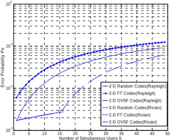
the special case of a Rician fading channel with R=0. In these two channels, the or-thogonality of the codes in the receiver’s side would be partially destroyed or all de-stroyed due to the effects of phase change and amplitude fading. Figs. 5 and 6 show error probabilities versus the number of si-multaneous users in a strong Rician fading and Rayleigh fading channels, where R=10 dB, SNR=10 dB. Figs. 7 and 8 show error

probabilities versus the number of simulta-neous users in a weak Rician fading and Rayleigh fading channels, where R=5 dB,

SNR=10 dB. From Figs. 5-8, we can find

that the difference among the performance of these three codes will decrease as R de-creases. In the extreme case (the Rayleigh fading channel), the performance of these three codes are almost the same.

2.5 Conclusions

In this project, we proposed 2-D FT codes which use Walsh codes and modified m-sequences for frequency-hopping and Barker codes for time-spreading. We also provided the performance analysis of 2-D FT codes, 2-D OVSF codes, and 2-D random codes under the AWGN, Rayleigh fading, and Rician fading channels. The results of our analysis showed that the proposed 2-D FT codes can support more number of sub-scribers than the 2-D OVSF codes with trade-off of the system performance.

3. 下一世代無線行動接取技術-子計畫三:

時空信號處理及多用戶檢測

3.1 Introduction

Much research on spatial and temporal signal processing using an adaptive antenna array has been pursued in recent years[8]-[13]. The LMS algorithm requires less computation and its significant feature is simplicity, while the RLS algorithm pro-vides a much faster convergence, and is relatively independent of the eigenvalues spread compared to the LMS algorithm [2]. Therefore, we will propose symbol-based adaptive antenna receiver structures without the need of calculation of the correlation matrix in this paper. We consider an MIMO-OFDM-DS/CDMA communication system similar to [14], which utilizes a transmit antenna array at the BS and a re-ceive antenna array at the MS. However, our work is different from [14] because our adaptive receiver operates the transmit array, receiver antenna array, and OFDM block in multipath fading environments.

3.2 System Model

For MIMO-OFDM-DS/CDMA multiuser communication system including K users sharing a common frequency band, each user is assigned a unique spreading sequence

k

c composed of Q chips at chip interval c T which is equal to T /Q_b .

[

() ( )

]

,k 1, ,K 2 ) ( 1 L = L = k H Q k k k c c c c (13)

where the superscript H represents the Her-mitian transpose. In OFDM systems, a block of data of size Q where Q is a power of 2 is

transmitted as an OFDM symbol. The base-band signal transmitted from the k-th user can be represented as ( ) ( ) ( ) ( ) ( ( ) ) ( ( )) [ ]T K K H t n Q s n Q s n Q s n n L L 2 1 1 1 N , 1, t , + − + − = = =F c d s (14)

where F is the Fast Fourier transform (FFT) matrix. The IFFT matrix represents as

H

F [9]. d_k∈{±1 ± j} is the data bit

trans-mitted by k-th user under QPSK modulation, t means the tth transmitted antenna, and the superscript T means transpose. We consider a MIMO channel with N transmitted and M received antennas for a widely used discrete path physical model [15] and can be written as

( ) ( )

( ) ( )N H T p M R p N H T P p p M R Pa θ a θ A θ H A θ h H=_∑ = =1 , , (15)

where H is the channel matrix, aT( )θN ,

( )M R θ

a are array steering by transmitter and

receiver, respectively. The transmitter and receiver are coupled via P propagation paths with

{ }

θN ,p and

{ }

θM ,p as the spatial angles

seen by the transmitter and receiver, respec-tively. The Hp represents the channel

fad-ing coefficient from p-th path. We suppose this channel model contains the effect of in-ter chip inin-terference (ICI). L is the length of impulse response. So, we can construct a impulse response vector as

[

a1 a2 L aL

]

.

The channel H( can be rewritten as follows

⎥ ⎥ ⎥ ⎥ ⎥ ⎥ ⎥ ⎥ ⎥ ⎥ ⎥ ⎦ ⎤ ⎢ ⎢ ⎢ ⎢ ⎢ ⎢ ⎢ ⎢ ⎢ ⎢ ⎢ ⎣ ⎡ = L L L H H H H H H H H H H 0 0 0 0 0 0 0 0 0 0 2 1 2 1 2 1 L M O M M O M O O M O M M O L ( ₍₁₆₎

where H₁=a₁×H,l=1,LL. H~ is

normal-ized H( . Next, we represent the transmitted

signal matrix S(n) as follows ( ) [ ( ) ( ) ( )] ( ) ( ) ( ( ) ) ( ( ) ) ( ) ( ) ( ( ) ) ( ( ) ) ( ) ( ) ( ) ⎥⎥ ⎥ ⎥ ⎥ ⎦ ⎤ ⎢ ⎢ ⎢ ⎢ ⎢ ⎣ ⎡ + − + − + − + − + − + − = = Qn s Qn s Qn s n Q s n Q s n Q s n Q s n Q s n Q s n n n n N N N N L M O M M L L L 2 1 2 1 2 1 2 1 2 1 2 1 2 1 1 1 1 1 1 1 s s s S

[

( ) ( ) ( )

]

T Q n n n z z z1 2 L = ( )n q

z is the q-th chip time signal of S(n). We

rewrite transmitted signal matrix as

( ) ( )( ) ( ) ( ) ( )( ) ( ) ( ) Q , 1, q , 1 2 2 1 2 2 L L M M M M L = ⎥ ⎥ ⎥ ⎦ ⎤ ⎢ ⎢ ⎢ ⎣ ⎡ = − − − − − − n n n n n n n q q L q q q L q q z z z z z z S we make S_q( )n multiplied by H~ ( )n _q( )n ( )n q HS V R =~ +

where V(n) is the zero mean and white Gaussian noise. The sum of elements on the diagonal of Rq( )n is what we want. Make

( )n

q

x represent the sum of elements on the

diagonal of Rq( )n . The baseband signal

transmitted through channel can be repre-sented as xq( )n .

3.3 Narrowband Adaptive Receiver 3.3.1 LMS-Based Receiver

In this subsection, we propose a MIMO-OFDM-DS/CDMA adaptive antenna receiver. As we mentioned before, antenna array is a appropriate description to MIMO channel model. The weight vector of the adaptive antenna is denoted as

( )

[

( ) ( ) ( )k

]

H M k k k LMS, n = w0 w1 L w −1 w (17)

The received signal matrix as ( )n

[

x ( )n x ( )n xQ( )n

]

U = 1 2 L (18) Obviously, each element in the received signal matrix U(n) is QPSK signal. We get the despreader output sequence de,LMS,k( )n

and can be described as

( )n ( )n ( )n Q d LMSk H H k k LMS e, , =c FU w , / (19)

where de,LMS,k( )n is the received signal

se-quence of the desired user. The cost function of adaptive algorithm known as the complex LMS algorithm is the expected value of sig-nal error. So, the cost function can be repre-sented as follows: ( ) ( ) ( ) ( ) _⎥⎦⎤ ⎢⎣ ⎡ = ⎥⎦ ⎤ ⎢⎣ ⎡ ₋ = 2 , 2 , n e E Q n n n d E J k LMS k LMS H H k k LMS c FU w (20)

where d_k( )n represents the original

trans-mitted signal of the desired user at time in-stant n [10]. We assume that d_k( )n is known

in training period, and we call it as a pilot sequence which is transmitted before data transmission in most wireless communica-tion system. According to the derivacommunica-tion of the LMS algorithm, we can recompose the cost function (20) as the following

( )

[

( ) ( ) ( ) ( ) ( ) ( ) ( ) ( ) ( )n n ( )n Q Q n n n d Q n n n n E n e E k k H k LMS k LMS H H k k LMS e k LMS H H k k H k LMS k LMS d Fc U w w FU c w FU c Fc U w , , * , , 2 , , 2 , − − = ⎥⎦ ⎤ ⎢⎣ ⎡ ( ) ( )nd n

]

d_{k k}* + (21)

where "*" means conjugate. It is no doubt that JLMS is a complex value. In order to

adaptively update the weight of the proposed receiver, we make a weight differential op-eration for cost function. We compute the gradient of the above cost function and then obtain ( )n ( )n Q J k LMS k H k LMS LMS , , 2U F c e w =− ∂ ∂ ₍₂₂₎

where eLMS ,k( )n denotes the error for the

de-sired user. Then, the weight vecor of the proposed receiver can be updated as follows,

( ) ( ) k LMS LMS k LMS k LMS J n n , , , 1 w _w w ∂ ∂ − = + µ (23)

where µ is the step size.

3.3.2 Narrowband Adaptive Receiver with Code Adjustment

In this subsection, we propose a new idea about adaptive receiver. It is to apply adaptive operation on spreading code. In traditional CDMA system, spreading code is an invariant sequence with fixed coefficients ±1 and has strong orthogonally. When spreading code sequence was transmitted through fading channel, it’s orthogonally would be ruined. So, we set up a new struc-ture for code adjustment. The proposed re-ceiver structure bases on LMS algorithm updates not only the weight vector of the MIMO-OFDM-DS/CDMA adaptive antenna receiver but also updates the despreading code coefficients. The elements of the de-spreading code are no longer ±1. According to the code update operation, the spreading code vector of the desired user should be de-fined as ( )_n

[

( )( )_n ( )( )_n ( )k ( )_n

]

Q k k k LMS c c c c , = 1 2 L (24)

the cost function can be represented like

JLMSCA as following: ( ) ( ) ( ) ( ) ( ) ( ) ( )

[

( ) ( ) ( ) ( ) ( )n n ( )n Q Q n n n d Q n n n n E Q n n n d E J k k LMS H H k LMS k LMS H H k LMS k k LMS H k LMS k LMS H H k LMS k LMS H H k LMS k LMSCA d c F U w w FU c Fc U w w FU c w FU c , , , , * 2 , , , , 2 , , − − = ⎥⎦ ⎤ ⎢⎣ ⎡ ₋ = ( ) ( )nd n

]

d_{k k}* + (25)

Take gradient of the cost function by the code vector we obtain

( )n ( )n ( )n Q J k LMSCA k LMS H k LMS LMSCA * , , , 2FU w e c =− ∂ ∂ ₍₂₆₎

where eLMSCA,k denotes the error for the

de-sired user. The update equation of the weight vector for this receiver is the same as

( ) ( ) k LMS LMS w n k LMS k LMS J n n , _ , , 1 w 2 _w w ∂ ∂ − = + µ (27)

The update equation of the despreader vec-tor coefficients for this receiver is shown as follows ( ) ( ) k LMS LMSCA c n k LMS k LMS J n n , _ , , 1 c 2 _c c ∂ ∂ − = + µ (28) 3.3.3 RLS-Based Receiver

Generally, recursive least squares (RLS) filter is faster than LMS filter in aspect of convergence speed. However, it is a tradeoff between convergence speed and computa-tional complexity. The computation com-plexity of recursive least squares filter are more than LMS filter. The update equation of weight vector and code vector coeffi-cients for RLS algorithm will be derived in following paragraph. Just like what we de-fine in the above section, the weight vector for RLS algorithm is denoted as wRLS ,k( )n as

follow ( )

[

( )_{( )} ( )_{( )} ( )k _{( )}

]

H M k k k RMS, n = w0 n w1 n w −1n w _L

We get the despreader output sequence ( )n

de,RLS,k and can be described as

( )n ( )n ( )n Q d RLSk H H k k RLS e, , =c FU w ,

Define the least squares cost function as the following, ( ) ( ) ( ) ( )2 , 1 1 2 , i e Q n n i d J k RLS i n n i n i k RLS H H k k i n RLS − = = − ∑ ∑ = − = λ λ c FU w (29)

where λ is the forgetting factor, and eRLS ,k( )n

denotes the error vector for the desired user. In order to derive the weight update equa-tion for RLS algorithm, it is necessary to compute∂ _, =0 ∂ k RLS RLS J

w . Then, compute the

gradi-ent of the above cost function and then ob-tain

( ) ( ) ( )

[

( )i d ( )i Q

]

Q n i i J k k H k RLS H H k k n i i n k RLS RLS c F U w FU c Fc U w 2 2 2 , 1 , − = ∂ ∂ ∑ = − λ and make 0 , = ∂ ∂ k RLS RLS J w ( ) ( ) ( ) ( )i ( )i Q n i i k k H n i i n k RLS H H k k n i i n d c F U w FU c Fc U ∑ ∑ = − = − = ⇒ 1 , 1 λ λ (30)

The optimum weight of the adaptive filter ahs the form

( )n Q w( ) ( )n w n k RLS Φ z w 1 , − = (31)

where Φ_w( )n represents correlation matrix

and z_w( )n represents cross-correlation

vec-tor. Φ_w( )n and z_w( )n are described as the

following, ( ) ( ) ( ) M i H H k k n i i n w n UiFc c FU i I Φ =∑λ +δλ = − 1 (32) ( )n ( )i k k( )i H n i i n w U F c d z ∑ = − = 1 λ (33)

where IMis the M-by-M identity matrix and

δ is the regularization parameter. Using ma-trix-inversion lemma and the definition

( )n _w( )n w 1 − = Φ P , we obtain ( )n = 1

[

(n−1)− ( )n ( ) (n w n−1)

]

H H k w w w P k c FU P P λ (34) where ( ) _{( )} ( ) ( )_{( ) ( )} ( ) ( ) k H w H H k w k H k H w w n n n n n n n n c F U P FU c P c F U c F U P K = − + − = − − 1 1 1 1 1 λ λ (35)

is the Kalman gain vector. Substitute (33) into (21) we can get substituting (34) forP_w( )n , and using (35) we get

( )n RLSk(n ) wQ w( )n k RLS w K Ω w , = , −1+ where ( )n ( )n RLSk(n )Q H H k k w=d −c FU w , −1 Ω is the

prior estimation error.

3.4 Simulation Results and conclusion

In this section, we show some simulation results of our proposed adaptive receiver

structures, as Fig. 9 shown. Before revealing the simulation results, there are some pa-rameters about most following simulation results : uptx = 2 ∼ 4 (the user number in each transmitted antenna branch), N = 4 (transmitted antenna number), M = 8 (Re-ceived antenna number). Furthermore, the data bits are transmitted with QPSK modu-lation. For LMS-based receiver structures, the step sizes for weight update equation are chosen from 0.02 to 0.001, and the step sizes for code update equation are chosen from 0.001 to 0.0001. For RLS-based receiver structures, we set the forgetting factor λ as 1. The spreading code we use is a set of Gold sequences with length Q = 31. From Figs.10 to Fig. 11, we find that the performances of the proposed RLS-based receivers are better than that of LMS-based receivers. Obviously, the performances of the system go down with the user number increasing in each transmitted antenna branch and Ec/N0 de-creasing. The reason is the narrowband adaptive receiver with code adjustment can reduce the effect of ICI and with less noise enhancement effect. The simulation results also show that when the Wiener code filter is employed, the performance is always better than that without using it.

4. 下一世代無線行動接取技術-子計劃四:

同步、通道估計與內接收機設計

4.1 Introduction

Orthogonal frequency division multi-plexing (OFDM) is a popular modulation scheme for high-speed broadband wireless transmission [16], [17]. It popularity derives mainly from its capability to combat fre-quency selective fading as intersymbol in-terference (ISI) caused by multipath delay spread can be easily eliminated. The former adopts the Multiple Input Multiple Output (MIMO) technique to enhance the capacity, where MIMO refers to systems that have multiple transmit antennas and multiple re-ceive antennas. Depending on the MIMO channel condition, the capacity of MIMO system increases with the number of trans-mitter and receive antennas. Recent devel-opments in MIMO techniques promise a great boost in performance for OFDM sys-tems.

With all its merits, OFDM, however, is sensitive to the carrier frequency offset (CFO) caused by Doppler shifts or instabili-ties of and mismatch between transmitter and receiver oscillators [18]. Depending on the application, the offset can be as large as many tens subcarrier spacing, and is usually divided into integer and fractional CFO parts.

The presence of a fractional CFO causes reduction of amplitude of desired subcarrier and induces inter-carrier interference (ICI) because the desired subcarrier is no long sampled at the zero-crossings of its adjacent carriers' spectrum. If the fractional CFO part can be perfectly compensated, the residual

integer CFO does not degrade the signal quality but still results in circular shifts of the desired output, causing decision errors.

In this report, we extend Moose's ML CFO estimation algorithm for use in a mul-tiple-antenna environments, assuming two identical pilot symbols are available. In ad-dition, we extend the Yu and Su’s ML CFO estimation algorithm that uses multiple re-petitive pilot symbols.

4.2 System Model

Consider a frequency selective fading channel associated with a MIMO system of

MT transmit and MR receive antennas. The

equivalent time-domain baseband signal at the output of the ith receive antenna, yi[n], is

given by

(36) where {wi[n]} is a complex additive whit

Gaussian noise (AWGN) sequence and

(37) is the part of the OFDM signal received by the ith receive antenna contributed by the jth transmit antenna. Moreover,

.

Sj[k] represents the symbol carried by the

kth subcarrier at the jth transmit antenna.

.

Hi_,j[k] is the channel transfer function between the ith receive antenna and the jth transmit antenna at the kth subcarrier.

.

ε denotes the relative carrier frequency offset of the channel (the ratio of the actual

frequency to the intercarrier spacing).

.

D is the set of modulated subcarrier for j the jth transmit antenna.

.

E is the average energy allocated to the kth s subcarrier evenly divided across the transmit antennas.

.

{

hi_,j[n]

}

and

∑

− = − = 1_{0 ,} 2 , [ ] [ ] L n N kn j j i j i k h ne H π

are the channel impulse and frequency re-sponse between the ith receive antenna and the jth transmit antenna at the kth subcarrier.

.

L is the maximum channel memory of all MTMR SISO component channels.

Fig. 12 plots the transmission channel model for the ith receive antenna with respect to the MT transmit antennas. Rewriting (2.1) in matrix form [ ] [ ] [ ] [ ] [ ] [ ]⎟⎟ ⎟ ⎟ ⎟ ⎠ ⎞ ⎜ ⎜ ⎜ ⎜ ⎜ ⎝ ⎛ + ⎟ ⎟ ⎟ ⎟ ⎟ ⎠ ⎞ ⎜ ⎜ ⎜ ⎜ ⎜ ⎝ ⎛ = ⎟ ⎟ ⎟ ⎟ ⎟ ⎠ ⎞ ⎜ ⎜ ⎜ ⎜ ⎜ ⎝ ⎛ + ∈ ∑ n w n w n w e k H k H k H k H k H k H k H k H M E N n y n y n y R j T R R T T R M N k n j D k M M M M M T s M M L L M O M M L L M 2 1 ) ( 2 , 1 , , 2 2 , 2 1 , 2 , 1 2 , 1 1 , 1 2 1 ] [ ] [ ] [ ] [ ] [ ] [ ] [ ] [ 1 π ε (38) and using the substitutions

we obtain

(4)

Let εf and εi be respectively the frac-tional and integer parts of the CFO so that

i f ε ε ε = + and define [ ] [ ] [ ] ( ) _{[ ]} [ ] [ ] [ ] [ ] ( ) _{[ ]} [ ] [ ] 1 2 / 2 / 0 1 2 / 0 1 2 / 2 / 0 1 1 1 f i j f f i m D j m ki N j m n N j kn N s m D n T N j n N s i i n T N j n N j m k n N s n T s i i T E Y k H m S m e e W k M N E H k S k e M N E H m S m e e W k M N E H k S k M ε π ε ε π πε πε π ε ε ε ε ε ∈ ≠ − − _{+ +} − ∈ = − − = − + − = ⎛ ⎞ = ⎜ ⎟+ ⎝ ⎠ ⎛ ⎞ = − − _{⎜ ⎟} ⎝ ⎠ ⎛ ⎞ + _{⎜ ⎟}+ ⎝ ⎠ = − − ∑ ∑ ∑ ∑ ∑ [ ] [ ] 2 ( 1) / ( )( 1) / sin( ) 1 sin( / ) sin( ( )) 1 sin( ( ) / ) f f i m D j m ki j N N f f circular shift

reduction of the desired subcarrier

j N N f i j s T f i e N N E H m S m e e M N m k N ε πε π ε ε π πε πε π ε ε π ε ε ∈ ≠ − − − + − − ⎛ ⎞ ⎜ ⎟ ⎜ ⎟ ⎝ ⎠ + + − + + ∑ 144424443 1444442444443 [ ] ( ) / m k N ICI W k − ⎛ ⎞ ⎜ ⎟ ⎜ ⎟ ⎝ ⎠ + 144444444444444424444444444444443 (39) It is clear that the presence of a fractional CFO causes reduction of the desired subcar-rier's amplitude and induces inter-carrier in-terference (ICI). If the fractional CFO part can be perfectly compensated for, the integer CFO, if exists, will result in a circular shift of the desired output, causing decision er-rors.

4.3 Maximum Likelihood Estimate of CFO

4.3.1 Generalized Moose Estimate

Let D be the set of modulated subcarrier (indexes) that bear a pseudonoise (PN) se-quence on the even frequencies and zeros on the odd frequencies. The resulting time-domain training sequence has two identical halves

[ ]

_∑

∈ + = e D k N k n j T s e k S k H M E N n r 1 [ ] [ ] 2π ( ε)/ (40) [ ] [ ] [ ] ( ) [ ] [ ] ( ) ( ) [ ] 2 ( / 2) / 2 / 2 / 2 2 / 2 1 / 2 1 , 1, 2 , / 2 j n N k N s m D T N j k N j n k N s m D T j E r n N H k S k e N M E H k S k e e N M r n e n N ε ε π ε π ε π ε πε + + ∈ + + ∈ + = = = =

∑

∑

K

(41) where

(

)

T M n r n r n r R[ ] ] [ ] [ ₂ 1 L and De is

the subset of even numbers in D.

Taking into account the AWGN term, we obtain

[ ]

n r[n] w[n] y = + (42)

[

/2

]

[ ] 2 /2 [ /2] N n w e n r N n y + = j πε + + (43) where

(

)

T M n w n w n w R[ ] ] [ ] [ ₂ 1 L . As

illustrated in Fig 13, we define

and

where the subscript indicates either the first or the second half of a time-domain OFDM frame and the indexes within the bracket denotes from which receive antenna the time domain sample is derived. (42) and (43) then have the simplified expressions

(44)

(45) The ML estimate of the parameterε , given the received vector

(

y₁[i],y₂[i]

)

, is

ob-tained by maximizing the likelihood func-tion

(

y₁[i],y₂[i]|ε

)

f

(

y₂[i]|y₁[i],ε

) (

f y₁[i]|ε

)

f =

(46)

where we have denoted various conditional probability density functions by similar functional expressions, f(.|.). Asε gives no

explicit information about y₁[i] , i.e.

(

y₁[i]|

)

f

(

y₁[i]

)

f ε = , the ML estimate of ε is given by

(

) (

)

(

ε

)

ε ε ε ε ε ], [ | ] [ max arg | ] [ ], [ | ] [ max arg ˆ 1 2 1 1 2 i y i y f i y f i y i y f = = (47) Since ) ] [ ] [ ( ] [ ] [ ]) [ ] [ ( ] [ 2 / 2 2 1 2 / 2 1 2 2 / 2 1 1 2 πε πε πε j j j e i w i w e i y i w e i w i y i y − + = + − = (48)

and w₁[i],w₂[i] are temporally white

Gaussian with zero mean and variance σ_w2I,

where I is the identity matrix, the multivari-ate Gaussian vector y₂[i] have mean

2 / 2 1[] πε j e i y

and covariance matrix

(49) Then ( )

(

[ ] [ ] [ ] [ ] [ ] [ ]

)

[ ] [ ]

(

)

(

[ ] [ ]

)

[ ] [ ]

{

}

1 1 2 2 1 1 2 / 2 2 / 2 2 1 2 1 2 1 2 / 2 2 1 2 1 * 2 / 2 2 1 1 1 , 1 | 1 , 1 exp 2 1 exp 2 2 1 = exp [ ] [ / 2] R R R R R R R M H j j i M H j i M M j i i i n f y y M y y M y y M y i y i e y i y i e y i y i e y n y n N e πε πε ω πε ω πε ω ε ε σ σ σ = − = − = = Λ = ⎧ ⎫ ∝ ⎨− − − ⎬ ⎩ ⎭ ⎧ ⎫ ∝ ⎨ ℜ ⎬ ⎩ ⎭ ⎧⎛ ⎞ ⎫ ⎪ ℜ⎨⎜ + ⎟ ⎪⎝ ⎠ ⎩

∑

∑

∑∑

L L L ⎧ ⎫ ⎪ ⎪⎪ ⎨ ⎬⎬ ⎪ ⎪ ⎭⎪ ⎩ ⎭ (50)

The ML estimate of ε is given by

(51)

where Arg(x) is the principal argument of the complex number x. In summary, the generalized Moose estimate for two identi-cal halves pilot symbols of length Nw and ND-spaced, as shown in Fig. 14, is given by

(52) The range of this estimator is

D N N 2 ± sub-carrier spacing. 4.3.2 Extended Yu Estimate

Consider a MIMO-OFDM system that uses multiple identical pilot symbols. After discarding the first received symbol, the re-maining K pilot symbols at the ith receive antenna, yi(k,m), can be represented as

) , ( ) , ( ) , (k m x k m w k m y_i = _i + _i (53)

for k=1,2,…,K and m=1,2,….,M where

xi(k,m) is the mth sample of the kth

(time-domain) symbol of the channel output at the ith receiver antenna. {wi(k,m)} are

uncorrelated circularly symmetric Gaussian random variables at the ith receive antenna with zero mean and variance

(

)

{

2

}

2 _{, m} k w E _i w = σ . Note that

(

)

( )

j (k )M N i k m x m e x , = ₁1, 2π −1 ε/ (54)

where ε is the relative frequency offset of the channel. Let

(55) where (.)T denotes the matrix transpose.

( ) ( )

m Aε

Y_i , and W_i

( )

m are the vectors of

dimension Kx1. Then, as shown in Fig 15, we have

( )

m A

( ) ( )

x m W

( )

m m M

Y_i = ε _i 1, + _i , =1,..., (56)

The received samples can thus be expressed compactly as

( )

i i i A X W Y = ε + (57) where Y_i =

[

Y_i

( )

1_LY_i

( )

M

]

is an KxM ma-trix. X_i =

[

x_i

( )

1 L,1 x_i

(

1,M

)

]

is an 1xM vector and W_i =

[

W_i

( )

1_LW_i

( )

M

]

is an KxM

matrix. Since the noise is temporally whit Gaussian, Yi(m) is a multivariate Gaussian

distributed random vector with covariance matrix σ_w2I. The joint ML estimates of A

and Xi, treating Xi as a deterministic

un-known vector, are obtained by maximizing the following joint likelihood function:

(

)

(

( )

( )

)

( ) ∑ ∑ ∝ Π Π = = = − − = = R M i M m i i w R R R m Ax m Y i i M m M i M M e m x A m Y f X X A Y Y f 1 1 2 2 _{(1, )} 1 1 1 1 1 | , | , 1, σ L L

The corresponding log-likelihood function, after dropping constant and unrelated terms, is given by

( )

(

)

=

∑ ∑

_{= =}

( )

−

( )

Λ MR i M m i i i m Y m Ax m x A ₁ 1 2 , 1 , 1 , (58)

For a given A, setting

( )

( )

1, 2 0 ) , 1 ( − = ∇ Y_i m Ax_i m m i x , we obtain

the conditional ML estimate,

( )

m x

( )

m AY

( )

m xi LS_i i + = = 1, , 1 ˆ ,where K A

A+ = H / and H denotes the Hermitian

operation. By substituting the least-square solution, x

( )

m i LS 1, , we obtain

(

)

2 2 1 1 1 1 1 1 1 1 ( ) ( ) ( ) ( ) ( ) ( ) ( ) ( ) ˆ R R R R M M M M i i A i i m i m M M M M H H i A i A i i i m i m R A YY A Y m AA Y m P Y m Y m P Y m tr P Y m Y m M Mtr P R + ⊥ = = = = ⊥ ⊥ = = = = ⊥ Λ = − = ⎛ ⎞ = _{= ⎜ ⎟} ⎝ ⎠ =

∑∑

∑∑

∑∑

∑∑

(59) where tr(.) denotes the trace of a matrix,

( ) ( )

∑ ∑

= = = R i M i H M m i R YY Y mY m M M R 1 1 1 ˆ _{, and} + ⊥ _{= −} AA I

PA . The desired CFO estimate is then given by

(

)

{

}

{

(

)

}

{

A R A

}

R P tr R P tr YY H YY A YY A ˆ max arg ˆ max arg ˆ min arg ˆ ε ε ε ε = = = ⊥ (60)

Invoking an approach similar to that used by the MUSIC algorithm, we set j M N

e z= 2πε /

and define the parametric vector

( )

[

1 2 _K 1

]

T, z z z z A = _L − (61)

so that the log-likelihood Λ = AHRˆ_YYA can

be expressed as a polynomial of order 2K-1,

( )

( )

ˆ

( )

1

( )

, ) 1 (

∑

− − − = = = Λ K K n n YY H z n s z A R z A z (62) where

( )

=

∑

j i YY i j R n s , ) , (

ˆ _{, for n=j-i, and}

n=-K+1,….,K-1. As the log-likelihood is a

real smooth function of ε , taking derivative of

(

j M N

)

e 2πε /

Λ with respect to ε and set-ting _∂Λ

(

j2πεM/N

)

_{∂ε =Λ}.

( )

_{ε =}0 e , we obtain

( )

₋ *( )₌0 z F z F (63) where

( )

∑

− = = 1 1 ) ( K n n z n ns z F is a polynomial

of order K-1. If {zi}are the nonzero complex

roots of

( )

z

.

Λ then the desired estimate is given by z M j N _ˆ ln 2 ˆ π ε = (64)

where zˆ arg{max

( )

z}

i

z Λ

=

We summarize the above ML estimation procedure as following.

1. Collect K received symbols from all

re-ceive antennas and construct the sample correlation matrix Rˆ , which is given by _YY

( ) ( )

∑ ∑

= = = R i M i H M m i R YY Y mY m M M R 1 1 1 ˆ _.

2. Calculate the coefficients of F(z) based on

YY Rˆ where

( )

∑

− = = 1 1 ) ( K n n z n ns z F , and

( )

=

_∑

j i YY i j R n s , ) , ( ˆ _{for n=j-i.}

3. Find the nonzero unit-magnitude roots of

( )

₋ *( )₌0

z F z

F .

4. Obtain the CFO estimate from

and z M j N _ˆ ln 2 ˆ π ε = and

( )

} max arg{ ˆ z z i z Λ = where

( )

z = A

( )

z HRˆ_YYA

( )

z Λ ,

( )

[

_K

]

T z z z z A = 1 2 _L −1 , N M j e z= 2πε / .

The range of our estimator is subcar-rier spacings.

4.4 Simulation Results and Discussion

The computer simulation results reported in this section are obtained by using a pilot format the same as the IEEE 802.11a stan-dard with a sample interval of 50 ns. The frequency-selective fading channel has six-teen paths with independent complex Gaus-sian distributed amplitudes and a exponen-tially decaying power delay profile with rms delay spreads of 50 ns. The tap coefficients are normalized such that the sum of the av-erage power per channel is unity. The DFT size is N = 64. The signal-to-noise ratio (SNR), defined as the ratio of the received

signal power (from all MT transmitters) to the noise power at the ith receive antenna, is assumed to be the same for each receive an-tenna. For Moose estimate, the training part consists of two identical halves with length

NW = 32. The range of CFO estimator is ± 1

subcarrier spacings. Fig. 16 shows the per-formance of generalized Moose CFO esti-mate for different number of transmit and receive antennas. Obviously, the MSE per-formance improves as the number of receive antennas, MR, increases. Fig. 17 presents the

performance of extended YS estimate for different number of transmit and receive an-tennas. The training symbol has two identi-cal halves with K = 2 and M = 32. The range of CFO estimator is 1± subcarrier spacings. For training symbol with two identical repe-tition, the performance of extended Yu esti-mate is the same as the performance of gen-eralized Moose's CFO estimate. Fig. 18 plots the performance of generalized Moose's CFO estimate with two identical halves with length NW = 32 for different

number of transmit and receive antennas. Similarly, the performance of CFO estimates is an increasing function of the number of the receive antennas. We divide roughly into four groups. The first group is MR = 1; MT =

1; 2; 4; 8, the second is MR = 2;MT = 1; 2; 4;

8 and so on. For first group, the performance of CFO estimate with MR = 1; MT = 8 is

bet-ter than with MR = 1; MT = 1 duo to transmit

diversity. The last group with MR = 8 is more close together than the first group with

MR = 1 duo to receive diversity. The

per-formance of CFO estimate for the second group, MR = 2, is roughly 3dB better than for

the first group, MR = 1, duo to two receive

antennas received double energy than single receive antenna. Fig. 19 shows the perform-ance of extended Yu estimate and general-ized Moose estimate. The training symbols have 4 repetitions with K = 4 and M =16. The training symbols for generalized Moose estimate are length NW = 32 i.e. take first

two training symbols as one training symbol and take last two training symbols as one training symbol. The range of generalized Moose's CFO estimator is 1± subcarrier spacings. The range of extended Yu estima-tor is ± subcarrier spacings. For 4 repeti-2 tions, the performance of extended YS mate is better than generalized Moose esti-mate because extend Yu estiesti-mate use all in-formation of training symbols.

4.5 Conclusion

In this project, we have extended both Moose's and Yu's maximum likelihood CFO estimation algorithms for use in MIMO-OFDM systems. As long as the length of cyclic prefix is greater than or equal to the maximum delay that accounts for the all users' timing ambiguities and channel multipath delays. The performance of both CFO estimates improves as the number of transmit/receive antennas in-creases. In other words, the presence of mul-tiple antennas not only promise great capac-ity enhancement but entail performance im-provement for the associated frequency synchronization subsystem.

5. Reference

[1] S. M. Tseng and M. R. Bell, “Asyn-chronous multicarrier DS-CDMA using mutually orthogonal complementary

sets of sequences,” IEEE Trans.

Com-mun., vol. 48, no. 1, pp. 53-59, Jan.

2000.

[2] C.-M. Yang, G.-C. Yang, P.-H. Lin and W. C. Kwong, “2-D orthogonal spreading codes for multi-carrier DS- CDMA systems,” Proc. of IEEE

ICC’03, May 2003, vol. 5, pp. 3277-

3281.

[3] G.-C. Yang and W. C. Kwong, Prime

Codes with Applications to CDMA Op-tical and Wireless Networks, Boston,

MA: Artech House, 2002.

[4] A. W. Lam and S. Tantaratana, Theory

and Application of Spread Spectrum Systems. Piscataway, NJ: IEEE, 1994.

[5] M. Pureley, “Performance evaluation for phase-coded spread-spectrum mul-tiple-access communication-Part I: System Analysis,” IEEE Trans.

Com-mun., vol. 25, pp. 795-799, Aug. 1977.

[6] M. Pursley and D. Sarwate, “Perform-ance evaluation for phase-coded spread-spectrum multiple-access com-munication-Part II: Code Sequence Analysis,” IEEE Trans. Commun., vol. 25, pp. 800-803, Aug. 1977.

[7] C.-P. Hsieh, C.-Y. Chang, G.-C. Yang, and W.C. Kwong, “A bipolar-bipolar code for asynchronous wavelength- time optical CDMA,” to appear in

IEEE Trans. Commun.

[8] R. A. Monzingo and W. T. Miller, lntro-duction to Adaptive Arrays, Wiley, 1980.

[9] S. Haykin, Adaptive Filter Theory, Pren-tice Hall, NJ, 2001.

[10] B. D. V. Veen and K. M. Buckley, "Beamforming: A Versatile Approach to Spatial Filtering," IEEE ASSP Mag., pp. 4-24, Apr. 1988.

[11] D. H. Johnson and D. E. Dudgeon,

Ar-ray Signal Processing: Concepts and Techniques, Prentice Hall, 1993.

[12] J. Litva and T. K-Y. Lo, Digital

Beam-forming in Wireless Communications,

Artech, 1996.

[13] J. S. Thompson, P. M. Grant, and B. Mulgrew, "Smart Antenna Arrays for CDMA Systems," IEEE Pers.

Com-mun., vol. 3, no. 5, Oct. 1996, pp.

16-25.

[14] Ruly Lai-U Choi, Ross D. Murch, and Khaled Ben Letaief, “MIMO CDMA Antenna System for SINR Enhance-ment” IEEE Trans. on Wireless

Com-mun., VOL. 2, NO. 2, MARCH 2003

[15] J. C. Liberti and T. S. Rappapor, Smart

Antennas for Wireless Communica-tions: IS-95 and Third Generation CDMA Applications, Prentice Hall, NJ,

1999.

[16] S. Weinstein, P. Ebert, “Data Transmis-sion by Frequency-DiviTransmis-sion Multiplex-ing UsMultiplex-ing the Discrete Fourier Trans-form," IEEE Trans. Commun., vol. 19, pp. 628 - 634, Oct 1971.

[17] R. van Nee, G. Awater, M. Morikura, H. Takanashi, M. Webster, and K. Halford, “New high-rate wireless LAN stan-dards," IEEE Commun. Mag., vol. 37, pp. 82-88, Dec. 1999.

[18] T. Pollet, M. Van Bladel, M. Moene-claey, “BER sensitivity of OFDM sys-tems to carrier frequency offset and Wiener phase noise," IEEE Trans.

Commun., vol. 43, pp. 191-193,

6. Tables and Figures 2 2 2 2 2 (Mv N )MPT_b g N σ σ + ( ) 2 2 ₁ b MPT K N σ − 2 2 2 (v )MPT_b (K 1) N σ + − 2 2 2 2 g b M PT N σ ( ) 2 ₁ b MPT K N −

*A Rayleigh fading channel is the special case of a Rician fading channel with v=0.

Table I

The variances of MAI of the 2-D FT codes, 2-D OVSF codes and 2-D random codes under the different channels.

) cos( 2P ω₁t ) cos( 2P ω₂t ) cos( 2P ω_Mt ) ( 1 , t C_k ) ( 2 , t C_k ) ( , t C_kM ) (t bk

×

×

×

×

×

×

Fig. 1 A transmitter model.

)

(t

r

1 ,1 2 cos(ω φt+ k) 2 ,2 2 cos(ω φt+ k ) , 2 cos(ω_Mt+φ_{k M}) ,1( ) k C t ,2( ) k C t , ( ) k M C t

×

×

×

×

×

×

b iT t= b iT t= b iT t= 1 Z 2 Z M Z Z

Fig. 2 A receiver model.

0 5 10 15 20 25 30 35 40 45 50 10-6 10-5 10-4 10-3 10-2 10-1 100

Number of Simultaneous Users K

E rr o r P robab ili ty P e 2-D Random Codes(Analysis) 2-D FT Codes(Analysis) 2-D OVSF Codes(Analysis)

Fig. 3 Error probability Pe versus number of

simultaneous users K for the three codes in an AWGN channel (N=7, SNR=10 dB). 0 5 10 15 20 25 30 35 40 45 50 10-6 10-5 10-4 10-3 10-2 10-1

Number of Simultaneous Users K

E rr o r P robab ili ty P e 2-D Random Codes(Analytic) 2-D FT Codes(Analytic) 2-D OVSF Codes(Analytic)

Fig. 4 Error probability Pe versus number of

simultaneous users K for the three codes in an AWGN channel (N=13, SNR=10 dB). 0 5 10 15 20 25 30 35 40 45 50 10-5 10-4 10-3 10-2 10-1 100

Number of Simultaneous Users K

E rr o r P robab ili ty P e 2-D Random Codes(Rayleigh) 2-D FT Codes(Rayleigh) 2-D OVSF Codes(Rayleigh) 2-D Random Codes(Rician) 2-D FT Codes(Rician) 2-D OVSF Codes(Rician)

Fig. 5 Error probability Pe versus number of

simultaneous users K for the three codes in the strong Rician fading and Rayleigh fading channels (N=7, R=10 dB, SNR=10 dB).

0 5 10 15 20 25 30 35 40 45 50 10-3

10-2 10-1 100

Number of Simultaneous Users K

E rr o r P robabi lit y P e 2-D Random Codes(Rayleigh) 2-D FT Codes(Rayleigh) 2-D OVSF Codes(Rayleigh) 2-D Random Codes(Rician) 2-D FT Codes(Rician) 2-D OVSF Codes(Rician)

Fig. 6 Error probability Pe versus number of

simultaneous users K for the three codes in the strong Rician fading and Rayleigh fading channels (N=13, R=10 dB, SNR=10 dB). 0 5 10 15 20 25 30 35 40 45 50 10-5 10-4 10-3 10-2 10-1 100

Number of simultaneous Users K

E rro r P e o b a b ili ty 2-D Random Codes(Rayleigh) 2-D FT Codes(Rayleigh) 2-D OBSF Codes(Rayleigh) 2-D Random Codes(Rician) 2-D FT Codes(Rician) 2-D OVSF Codes(Rician)

Fig. 7 Error probability Pe versus number of

simultaneous users K for the three codes in the weak Rician fading and Rayleigh fading channels (N=7, R=5 dB, SNR=10 dB). 0 5 10 15 20 25 30 35 40 45 50 10-3 10-2 10-1 100

Number of Simultaneous Users K

Er ro r Pr o b a b ili ty Pe 2-D Random Codes(Rayleigh) 2-D FT Codes(Rayleigh) 2-D OVSF Codes(Rayleigh) 2-D Random Codes(Rician) 2-D FT Codes(Rician) 2-D OVSF Codes(Rician)

Fig. 8 Error probability Pe versus number of

simultaneous users K for the three codes in the weak Rician fading and Rayleigh fading channels (N=13, R=5 dB, SNR=10 dB).

Fig. 9 MIMO-OFDM-DS/CDMA Receiver Structures

Fig. 10 BER performance of narrowband LMS-based adaptive receiver with different user number in each transmitted antenna branch.

Fig. 11 BER performance of narrowband RLS-based adaptive receiver with different user number in each transmitted antenna branch.

Fig. 12 Channel model for the ith receive antenna.

Fig. 13 Definitions of various vector nota-tions.

Fig. 14 The ND-spaced estimator.

Fig. 9 Symbol arrangement and definitions of the extended Yu's ML estimate at the ith receive antenna.

Fig. 10 MSE performance of generalized moose estimate for two repetitions, true CFO = 0:7 subcarrier spacings.

Fig. 11: MSE performance of extended Yu estimate for two repetitions, true CFO=0:7 subcarrier spacings.

Fig. 12: MSE performance of generalized moose estimate for two repetitions, true CFO=0:7 subcarrier spacings.

Fig. 13: MSE performance of CFO esti-mates for four repetitions, true CFO = 0:93 subcarrier spacings.