Optimization of parameter design: an intelligent approach using neural network and simulated annealing

This article was downloaded by: [National Chiao Tung University 國立交通大學] On: 28 April 2014, At: 00:09

Publisher: Taylor & Francis

Informa Ltd Registered in England and Wales Registered Number: 1072954 Registered office: Mortimer House, 37-41 Mortimer Street, London W1T 3JH, UK

International Journal of Systems Science

http://www.tandfonline.com/loi/tsys20

Optimization of parameter design: An

intelligent approach using neural network and

simulated annealing

Chao-Ton Su a & Hsu-Hwa Chang b a

Department of Industrial Engineering and Management , National Chiao Tung University , Hsinchu, Taiwan, ROC E-mail:

b

Department of Industrial Engineering and Management , National Chiao Tung University , Hsinchu, Taiwan, ROC

Published online: 26 Nov 2010.

To cite this article: Chao-Ton Su & Hsu-Hwa Chang (2000) Optimization of parameter design: An intelligent approach using neural network and simulated annealing, International Journal of Systems Science, 31:12, 1543-1549, DOI: 10.1080/00207720050217313

To link to this article: http://dx.doi.org/10.1080/00207720050217313

PLEASE SCROLL DOWN FOR ARTICLE

Taylor & Francis makes every effort to ensure the accuracy of all the information (the “Content”) contained in the publications on our platform. However, Taylor & Francis, our agents, and our licensors make no representations or warranties whatsoever as to the accuracy, completeness, or suitability for any purpose of the Content. Any opinions and views expressed in this publication are the opinions and views of the authors, and are not the views of or endorsed by Taylor & Francis. The accuracy of the Content should not be relied upon and should be independently verified with primary sources of information. Taylor and Francis shall not be liable for any losses, actions, claims, proceedings, demands, costs, expenses, damages, and other liabilities whatsoever or howsoever caused arising directly or indirectly in connection with, in relation to or arising out of the use of the Content.

This article may be used for research, teaching, and private study purposes. Any substantial or systematic reproduction, redistribution, reselling, loan, sub-licensing, systematic supply, or distribution in any form to anyone is expressly forbidden. Terms & Conditions of access and use can be found at http://www.tandfonline.com/page/terms-and-conditions

Optimization of parameter design: an intelligent approach using

neural network and simulated annealing

C

-

T

S

_y

and

H

-

H

C

_y

Parameter design optimization problems have found extensive industrial applications, including product development, process design and operational condition setting. The parameter design optimization problems are complex because non-linear relationships and interactions may occur among parameters. To resolve such problems, engineers commonly employ the Taguchi method. However, the Taguchi method has some limita-tions in practice. Therefore, in this work, we present a novel means of improving the eVectiveness of the optimization of parameter design. The proposed approac h employs the neural network and simulated annealing, and consists of two phases. Phase 1 formulates an objective function for a problem using a neural network method to predict the value of the response for a given parameter setting. Phase 2 applies the simulated annealing algorithm to search for the optimal parameter combination. A numerical example demonstrates the eVectiveness of the proposed approach.

1. Introduction

The optimization of parameter design problems has been extensively performed in industry. Engineers fre-quently encounter parameter design problems, particu-larly in product development, process design and operational condition setting. Parameter design prob-lems are complex because non-linear relationships and interactions may occur among parameters. Although engineers conventionally apply the Taguchi method to resolve these problems (Phadke 1989, Fowlkes and Creveling 1995), the Taguchi method has some limita-tions in practice. First, this method can only ® nd the best one of the speci® ed parameter level combinations. Once the parameter levels are determined, the feasible solution space is constrained concurrently. Second, while only addressing the discrete control factor, the Taguchi method cannot obtain the optimal condition when the parameter values are continuous. Third, the adjustment factor cannot be guaranteed to exist in prac-tice. Fourth, for a new product development or process design, the Taguchi method uses screening experiments

to diminish the range of control factor levels, thereby decreasing the solving e ciency owing to an increasing number of experiments (Pignatiello 1988).

An alternative means of using the neural network has recently been proposed to improve Taguchi’s parameter design, capable of eŒectively treating continuous par-ameter values (Rowlands et al. 1996, Chiu et al. 1997, Tay and Butler 1997). However, the method cannot e -ciently obtain the optimal parameter combination.

To resolve the limitations of previous methods, this work presents an arti® cial intelligence-based technique which combines the neural network with simulated annealing (SA). Neural network is a mathematical model, capable of accurately representing a complex relationship between inputs and outputs. SA algorithm is a stochastic optimization technique, which adopts the strong analogy between the physical annealing process of solids and the process of solving optimization prob-lems (Khan et al. 1997).

The approach proposed herein has two phases. First, the neural network approach is applied to map out the relationship between inputs and outputs; the trained neural model is also used to accurately predict the response (output) at a given parameter setting (input). Second, the SA algorithm is applied (through the trained neural model) to search for the optimal response and the corresponding parameter setting. The searched parameter setting is not limited to a discrete value. In

International Journal of Systems Science ISSN 0020± 7721 print/ISSN 1464± 5319 online#2000 Taylor & Francis Ltd http://www.tandf.co.uk/journals

Accepted 26 October 1999.

{ Department of Industrial Engineering and Management, National Chiao Tung University, Hsinchu, Taiwan, ROC.

* To whom correspondence should be addressed. E-mail:

ctsu@cc.nctu.edu.tw Accepted 26 October 1999.

addition, we do not need to utilize the adjustment fac-tors to adjust the process mean. Moreover, it is more e cient in obtaining the optimum than previous methods. Furthermore, a numerical example demon-strates the eŒectiveness of the proposed approach.

The rest of this paper is organized as follows. Section 2 describes the operating process of the neural network. Section 3 introduces the SA algorithm. Section 4 pro-poses a method that combines the neural network with the SA algorithm to resolve parameter design problems. Section 5 presents an illustrative example from previous literature to demonstrate the eŒectiveness of the pro-posed approach. Concluding remarks are ® nally made in Section 6.

2. Neural network

Neural network is a mathematical model, consisting of many processing elements connected from layer to layer. Each processing element (node) has an output signal that fans out along connections to each of the other processing elements. Each connection is assigned a rela-tive weight. A node’s output depends on the speci® ed threshold and the transfer function. Learning and recal-ling are two major processes of the neural network, where the learning process can modify the connecting weights and the recalling process involves understanding how the network creates a response at the output layer by processing a signal through the whole network. Two types of learning are commonly addressed: supervised and unsupervised learning. For supervised learning, a set of training input vectors with a corresponding set of target vectors is trained to adjust the weights in a neural network. For unsupervised learning, although a set of input vectors is proposed, no target vectors are speci® ed. Generally, the clustering problem frequently employs the unsupervised learning and the prediction or mapping problem usually employs the supervised learning.

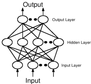
Our approach to solving Taguchi’ s parameter design problem is based on the supervised neural network. A backpropagatio n neural network is commonly used among the several well-known supervised learning net-works, e.g. learning vector quantization and counterpro-pagation neural networks. Herein, we adopt the backpropagatio n neural network owing to its ability to map a complex non-linear relationship between the inputs and the corresponding outputs (Funahashi 1989). A typical backpropagatio n network consists of three or more layers, including an input layer, one or more hidden layers and output layer. Figure 1 illustrates the topology of a backpropagatio n network with three layers. Backpropagation learning employs a gradient-descent algorithm to minimize the mean-square error between the target data and the predictions of the

neural network (Rumelhart and McClelland 1989). The training data set is initially collected to develop a backpropagatio n neural network model. Through a supervised learning rule the data set comprises of an input and an actual output (target). The gradient-des-cent learning algorithm enables a network to enhance its performance by self-learning. The training of a back-propagation network involves three stages: the feedfor-ward of the input training data, the calculation and backpropagatio n of the associated error, and the adjust-ment of the connected weights. The equation utilized to adjust the weights for the output layer k is

Wkjˆ ²¯koj

where W_kj ˆ the change to be made in the weight from the jth to kth unit.

²ˆ the learning rate

¯kˆ the error signal for unit k

ojˆ the jth value of the output pattern The backpropagatio n rule for changing weights for the hidden layer j is

W_jiˆ ²¯joi

where W_jiˆ the change to be made in the weight from the ith to jth unit

²ˆ the learning rate

¯_jˆ the error signal for unit j

oiˆ the jth value of the output pattern The detailed operating process is given as follows (Fausett 1994).

Step 1. Initialize the weights between layers.

1544 C.-T. Su and H.-H. Chang

Output

Input

Figure 1. Topology of the backpropagation neural network.

Step 2. Select the learning schedule (e.g. set the transfer function, learning rate, momentum, learning count).

Step 3. Repeat steps 4± 10 until learning counts or the error criterion has arrived.

Feedforward:

Step 4. Each input node receives input data and passes this data to all nodes in the next layer.

Step 5. Each hidden nodes sums up its weighted input data, applies the transfer function to compute its output data and, then, sends these data to all nodes in the next layer.

Step 6. Each output nodes sums up its weighted input data, then applies the transfer function to com-pute its output data.

Backpropagation of error:

Step 7. Each output node receives a target data cor-responding to the input training data, computes its error term, calculates its weight correction term and, then, sends the error term to nodes in the previous layer.

Step 8. Each hidden node sums up its weighted input error term, computes its error term, calculates its weight correction term and, then, sends the error term to nodes in the previous layer. Update weights:

Step 9. Each output node updates its weights. Step 10. Each hidden node updates its weights.

3. Simulated annealing

Simulated annealing (SA), which was introduced by Kirkpatrick et al. (1983) and independently by Cerny (1985), has been applied to various di cult combina-torial optimization problems. SA is a stochastic opti-mization technique, which derives from an analogy between the annealing process of solids and the strategy of solving optimization problems. SA is a type of local search algorithm, but with the added advantage of not being trapped in local optima (Eglese 1990). Starting from an initial solution, SA generates a new solution x0 in the neighbourhood of the current solution x. Then, calculate the change in the objective function, i.e. Eˆ f …x0_{† ¡ f …x†. In}

mini-mization problems, if E < 0, transition to the new solution is accepted. If E¶ 0, then transition to the new solution is accepted with a speci® ed probability obtained by the function e¡ E=T, where T is a control parameter called the temperature. SA repeats this pro-cess M times at each temperature, where M is a con-trol parameter called the epoch length. The value of T is gradually decreased by a cooling function. The

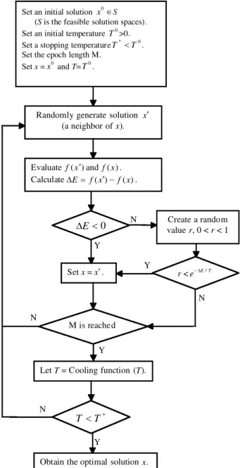
typical procedure for implementing a SA algorithm is shown in ® gure 2 (Koulamas et al. 1994, Park and Kim 1998).

To implement an SA algorithm to a speci® c problem, we have to de® ne: (i) the con® guration of the possible solutions; (ii) neighbourhood of a solution; (iii) an objective function; (iv) the annealing schedule. In addi-tion, the annealing schedule consists of: (i) the initial temperature; (ii) a cooling function for decreasing the temperature; (iii) epoch length at each temperature; and (iv) a stopping condition to terminate the algorithm (Su and Hsu 1998).

Y N

Let T = Cooling function (T).

*

T T <

Obtain the optimal solution x. Set an initial solution x Î0 S

(S is the feasible solution spaces). Set an initial temperature 0

T >0. Set a stopping temperature_{T <}* _T0_. Set the epoch length M.

Set x =_x0 _{and T=T}0_.

Randomly generate solution x¢ (a neighbor of x). Evaluatef(x¢ and) f(x). CalculateD E= f(x¢)- f(x). 0 < D E Set x = x¢ . _{r <} E T e-D / Create a random value r, 0 < r < 1 M is reached Y N N Y Y N

Figure 2. The schema of the SA algorithm.

4. Proposed approac h

Taguchi’s parameter design method uses an orthogonal array to arrange the experiment for a particular prob-lem. The corresponding response can be obtained by the speci® ed parameter combination. Taguchi applies the signal-to-noise ratio to perform the response analysis. Next, the Taguchi method employs the two-step optimi-zation procedure to attain the best response and par-ameter combination. In this work, we propose an alternative means of resolving the above problems. The proposed approach applies a combined method using the backpropagatio n network and SA to analyse the parameter design problem. Figure 3 schematically depicts the proposed approach.

The proposed procedure consists of two phases. The ® rst phase in the proposed procedure involves identi-fying the objective function for a parameter design prob-lem. A backpropagatio n network is trained to derive the relationship between the control factor values and the responses. The trained network can accurately predict

the behaviour of possible control factor combinations. Thus, inputting the control factor values into the trained network allows us to obtain the corresponding response. The trained network is used as the objective function in the SA. In phase two, SA is directly applied to solve the problem. SA can be used to obtain the optimal value of the control factor from the possible solution spaces. Here, a possible solution is represented by a vector of parameter values. For instance, a system has ® ve par-ameters A, B, C, D, and E. A vector (9, 3, 6, 1, 4) can represent the values of the ® ve parameters (A, B, C, D, E), respectively. The de® nition of the neighbourhood of the vector is referred to the j-neighbourhood (Cheh et al. 1991). The j-neighbourhood of the vector means selecting any j parameters and then randomly assigning another setting for each of them. For instance, the 1-neighbourhood of vector (9, 3, 6, 1, 4) involves selecting a parameter (e.g. parameter C) and then assigning another setting (e.g. 5) to replace the value 6. In the instance, the neighbour of (9, 3, 6, 1, 4) is set as (9, 3, 5, 1, 4). The procedure of the proposed approach is given as follows.

Phase 1. Identify the objective function to predict the

response.

Step 1. Collect the training and testing patterns by randomly selecting the data from the ortho-gonal table.

Step 2. Develop a backpropagatio n network model to derive the relationship between control factor values and responses. This trained network is referred to herein as the objective function.

Phase 2. Determine the optimal control factor

combina-tion.

Step 3. Create an initial solution (x0) by randomly selecting the value of the control factors within the upper and lower bounds.

Step 4. Set an initial temperature T0> 0.

Step 5. Set xˆ x0, T ˆ T0, and de® ne the neighbour-hood structure.

Step 6. Set the epoch length M, and the cooling factor ¬, 0 < ¬ < 1.

Step 7. Repeat steps 8± 14 until a predetermined stop-ping temperature is reached.

Step 8. Repeat steps 9± 13 M times. Step 9. Randomly generate solution x0.

Step 10. Calculate the change of response

Eˆ f …x0† ¡ f …x†, where the objective func-tion f istaken from step 2.

Step 11. Generate a random value r. Step 12. If E < 0, then set xˆ x0_{, else}

if r < e¡ E=T, then set x ˆ x0. 1546 C.-T. Su and H.-H. Chang A backpropagation neural network Control factor value Response

Set operation condition: initial solution initial temperature

epoch length colling factor

Decrease the temperature No

Yes Determine the new solution

by the change of response

and a specified probability

Evaluate response (by a well-trained

back-propagation neural network)

Yes No Generate a neighbor solution

Evaluate the response Phase 1: Identify the objective function

Phase 2: Determine the optimal control factor combination

stop Obtain optimal combination _{and response}

M times

Figure 3. The schema of the proposed approach.

Step 13. Call the current parameter settings the optimal condition.

Step 14. Set Tˆ ¬T.

Step 15. Obtain the predicted response value by input-ting the optimal control factor value to the objective function.

5. Numerical example

This section presents a numerical example of a gas-assisted injection moulding process with a single response to demonstrate the proposed approach’s eŒec-tiveness (Hsu 1995). The response of this case is the length in the gas channel. This study attempts to make the response as small as possible by selecting parameter set values. Eight controllable factors were selected: mould temperature, melt temperature, injection speed, gas injection time, gas pressure, gas distance, gas delay

time and constant pressure time, and they were denoted by A, B, C, D, E, F, G and H, respectively. The Taguchi L18 orthogonal array was used to allocate the parameter

combinations. Table 1 lists the values of the parameter levels and the responses of the experiment. This numer-ical example is analysed again by our proposed approach.

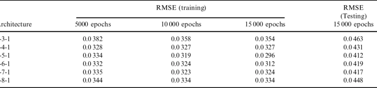
When Phase 1 is applied to this example, the training and testing patterns for the backpropagatio n network are initially formed. In this study, we randomly select 72 training patterns and 18 testing patterns from table 1. The control factor values and responses serve as inputs/ outputs of the network. A neural network package soft-ware, Qnet97 (1997), is used to develop the required network. The convergence criterion employed in the net-work training is the root of mean square error (RMSE). Table 2 lists several options of the network architecture; in addition, the structure 8-5-1 is selected to obtain a

Table 1. Control factor values and responses of the experiment

Control factors Responses

A B C D E F G H y1 y2 y3 y4 y5 1 50 230 50 1 90 64 0 0 42 40 57 68 74 2 50 230 60 1.5 110 65 0.5 3 71 76 74 74 75 3 50 230 70 2 130 66 1 6 84 80 83 80 82 4 50 240 50 1 110 65 1 6 37 29 34 38 41 5 50 240 60 1.5 130 66 0 0 117 115 121 123 116 6 50 240 70 2 90 64 0.5 3 37 36 36 39 36 7 50 250 50 1.5 90 66 0.5 6 85 87 88 93 90 8 50 250 60 2 110 64 1 0 28 26 24 25 29 9 50 250 70 1 130 65 0 3 84 79 84 79 73 10 60 230 50 2 130 65 0.5 0 74 84 64 69 65 11 60 230 60 1 90 66 1 3 84 87 95 88 94 12 60 230 70 1.5 110 64 0 6 71 68 68 70 65 13 60 240 50 1.5 130 64 1 3 25 24 25 28 24 14 60 240 60 2 90 65 0 6 88 88 89 90 79 15 60 240 70 1 110 66 0.5 0 114 124 125 117 118 16 60 250 50 2 110 66 0 3 106 106 104 99 107 17 60 250 60 1 130 64 0.5 6 31 41 43 36 40 18 60 250 70 1.5 90 65 1 0 60 53 58 51 61

Table 2. The performance of six diŒerent networks.

RMSE (training) RMSE

(Testing)

Architecture 5000 epochs 10 000 epochs 15 000 epochs 15 000 epochs

8-3-1 0.0 382 0.0 358 0.0 354 0.0 463 8-4-1 0.0 328 0.0 327 0.0 327 0.0 431 8-5-1 0.0 334 0.0 319 0.0 296 0.0 412 8-6-1 0.0 332 0.0 324 0.0 312 0.0 419 8-7-1 0.0 335 0.0 323 0.0 324 0.0 417 8-8-1 0.0 344 0.0 334 0.0 334 0.0 448

better performance. At this moment, the trained net-work 8-5-1 is employed as the objective function of the SA which will be used in Phase 2.

In Phase 2, SA is performed. The algorithm is coded in C language and implemented on a Pentium 166 PC. The operational condition is set as follows.

(1) The eight parameter ranges are reasonably set as (45.0, 65.0), (220, 260), (45.0, 75.0), (0.85, 2.15), (80.0, 140.0), (63.0, 67.0), (0, 1.15) and (0, 7.0), re-spectively.

(2) The neighbourhood structure is 1-neighbourhood . (3) The initial temperature is 1.

(4) The stopping temperature is 0.001. (5) The epoch length M ˆ 20.

(6) The cooling factor ¬ ˆ 0:95.

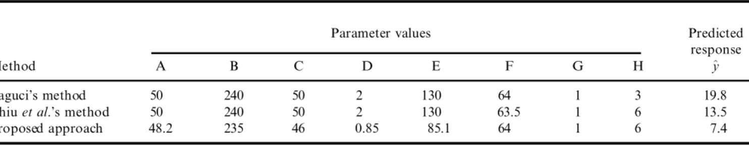
The above information is used and the SA program is executed over 20 runs to obtain the optimum settings (48.2, 235, 46, 0.85, 85.1, 64, 1, 6). Table 3 summarizes the implementation results. The smallest response is 7.4. Table 4 lists the optimal control factor values.

If the 18 original observations in table 1 are analysed using the Taguchi method, we have the optimum set-tings (50, 240, 50, 2, 130, 64, 1, 3) for the eight control factors (A, B, C, D, E, F, G, H), and the predicted response under this optimal condition is 19.8. In addi-tion, Chiu et al. (1997) proposed a neural network-based method to resolve the same problem. Table 4 compares the analysis results of their and our study. This table reveals that Chiu et al.’s approach and the Taguchi method only slightly diŒer in terms of the control factor settings. In addition, the parameter settings of

the proposed approach largely diŒer from the other two approaches. However, the proposed approach out-performs the Taguchi method and Chiu et al.’s approach. Correspondingly, the validity of the proposed approach is established.

6. Conclusions

Parameter design problems are di cult for engineers to develop products and processes because complex non-linear relationships may exist among the parameters and responses. Although conventionally employed to solve such problems, the Taguchi method cannot attain the optimal condition when the parameter values are con-tinuous. Moreover, a neural network-based method can conquer the continuous parameter values, which is occa-sionally ine cient in terms of obtaining the optimal con-dition. In this work, we present an e cient approach to overcome these problems. Based on arti® cial intelligence techniques, the proposed approach combines the neural network with the SA to optimize the parameter design. The proposed approach consists of two phases. The ® rst phase identi® es the ® tness function for the problem, while phase two directly applies SA to determine the optimal condition of the problem. A numerical example demonstrates the eŒectiveness of the proposed approach. The proposed approach possesses ® ve merits of considerable importance.

(1) The proposed approach can treat both quantitative parameters and qualitative parameters.

(2) The proposed approach can eŒectively deal with the interactions among the parameters.

(3) As long as the historical experimental data are su -cient, no additional experiments are necessary and the data can be directly applied to the proposed approach.

(4) The proposed approach is an improvement over previous parameter design techniques, and is more e -cient to ® nd the optimum.

(5) The proposed approach is relatively simple and is fairly easy for engineers to apply to diverse indus-trial applications.

1548 C.-T. Su and H.-H. Chang

Table 3. Implementation results of SA

Item Data

The smallest response in 20 runs 7.42

The largest response in 20 runs 7.47

Average ® nal response 7.44

Standard deviation 0.0 134

Average CPU time (s/run) 36

Table 4. A comparison of the analysis results

Parameter values Predicted

response

Method A B C D E F G H ^y

Taguci’s method 50 240 50 2 130 64 1 3 19.8

Chiu et al.’s method 50 240 50 2 130 63.5 1 6 13.5

Proposed approach 48.2 235 46 0.85 85.1 64 1 6 7.4

Restated, it does not require much statistical back-ground for engineers. In addition, applying the pro-posed approach allows engineers to directly use neural network software and SA program to optimize the prob-lems without any theoretical knowledge of neural com-puting and SA.

References

CERNY,V.,1985, Thermodynamical approach to the traveling sales-man problem, an e cient simulation algorithm. Journal of

Optimization Theory and Applications, 45, 41± 51.

CHEH,K.M.,GOLDBERG,J.B., andASKIN,R.G.,1991, A note on the eŒect of neighborhood structure in simulated annealing.

Computers and Operations Research, 18, 537± 547.

CHIU,C.-C.,SU,C.-T.,YANG,G.-H.,HUANG,J.-S.,CHEN,S.-C., and CHEN,N.-T.,1997, Selection of optimal parameters in gas-assisted injection moulding using a neural network model and the Taguchi method. International Journal of Quality Science, 2, 106± 120.

EGLESE,R.W.,1990, Simulated annealing: a tool for operational research. European Journal of Operational Research, 46, 271± 281. FAUSETT, L., 1994, Fundamentals of Neural Networks: An

Architectures, Algorithms, and Applications (location?: Prentice

Hall).

FOWLKES,W.Y., andCREVELING,C.M.,1995, Engineering Methods

for Robust Product Design: Using Taguchi Methods in Technology and Product Development (location?: Addison-Wesley).

FUNAHASHI,K.,1989, On the approximate realization of continuous mapping by neural network. Neural Networks, 2, 183± 192.

HSU,K.S.,1995, Fundamental study of gas-assisted injection mould-ing process. Thesis, Chung Yuang University, Taiwan.

KHAN,Z.,PRASAD,B., and SINGH,T.,1997, Machining condition optimization by genetic algorithms and simulated annealing.

Computers and Operations Research, 24, 647± 657.

KIRKPATRICK,S.,GELATT JR, C.D., and VECCHI,M.P.,1983, Optimization by simulated annealing. Science, 220, 671± 680. KOULAMAS,C.,ANTONY,SR., andJAEN,R.,1994, A survey of

simu-lated annealing applications to operations research problems.

Omega: Internationa l Journal of Management Science, 22, 41± 56.

PARK,M.W., andKIM,Y.D.,1998, A systematic procedure for set-ting parameters in simulated annealing algorithms. Computers and

Operations Research, 25, 207± 217.

PHADKE,M.S.,1989, Quality Engineering Using Robust Design (loca-tion?: Prentice Hall).

PIGNATIELLO,J.J.,1988, An overview of the strategy and tactics of Taguchi. IIE Transactions , 20, 247± 254.

Qnet97 (1997) Neural network modeling. Vesta Services.

ROWLANDS, H.,PACKIANATHER, M. S., and OZTEMEL,E.,1996, Using arti® cial neural networks for experimental design in oŒ-line quality. Journal of Systems Engineering, 6, 46± 59.

RUMELHART, D. E., and MCCLELLAND, J. L., 1989, Parallel

Distributed Processing: Explorations in the Microstructure of Cognition, Vol. I (Cambridge, MA: MIT Press).

SU,C.-T., andHSU,C.-M.,1998, Multi-objective machine-part cell formation through parallel simulated annealing. International

Journal of Production Research, 36, 2185± 2207.

TAY,K.M., andBUTLER,C.,1997, Modeling and optimizing of a MIG welding processÐ a case study using experimental designs and neural networks. Quality and Reliability Engineering International, 13, 61± 70.