900 IEEE TRANSACTIONS ON NEURAL NETWORKS, VOL. 5 , NO. 6, NOVEMBER 1994
A Parallel Geneticmeural Network Learning
Algorithm for MIMD Shared Memory Machines
S.
L. Hung and H. Adeli
Abstract-A new algorithm is presented for training of mul-
tilayer feedforward neural networks by integrating a genetic algorithm with an adaptive conjugate gradient neural network learning algorithm. The parallel hybrid learning algorithm has been implemented in C on an MIMD shared memory machine (Cray Y-MP8/864 supercomputer). It has been applied to two
different domains, engineering design and image recognition. The performance of the algorithm has been evaluated by applying it to three examples. The superior convergence property of the parallel hybrid neural network learning algorithm presented in this paper is demonstrated.
I. INTRODUCTION
UPERVISED learning algorithms have been investigated
S
and explored in several domains. The convergence speed of these algorithms is often slow. Several hours or even days of computer time are often required to train neural networks using the conventional serial workstations. In addition, the total number of iterations for learning an example in neu- ral networks is often in the order of thousands [l], [lo]. Thus, how to improve the learning performance of neural networks is currently an important research problem. One approach, inspired by the human brain neurons performing many operations simultaneously, is the development of learn- ing algorithms on general-purpose parallel computers with the objective of reducing the overall computing time [ll]. Hung and Adeli [12] present parallel backpropagation neural networks learning algorithms employing the vectorization and microtasking capabilities of vector MIMD machines. They report a maximum speedup of 6.7 using eight processors for a large network with 5950 links.Another approach is the development of more effective neural network learning algorithms with the objective of reducing the leaming time. For example, we have developed an adaptive conjugate gradient neural networks learning al- gorithm and applied it to the domains of engineering design and image recognition. The problem of arbitrary trial-and-error selection of the learning and momentum ratios encountered in the momentum backpropagation algorithm is circumvented in
Manuscript received September 21, 1992; revised July 26, 1993. This work has been supported in part by the National Science Foundation under Grant MSS-9222114.
S . L. Hung is with the Department of Civil Engineering, National Chiao Tung University, HsinChu, Taiwan 30050, R.O.C.
H. Adeli is with the College of Engineering, The Ohio State University, Columbus, OH 43210-1275 USA.
IEEE Log Number 9212202.
the new adaptive algorithm. Instead of constant learning and momentum ratios, the step length in the inexact line search is adapted during the learning process through a mathematical approach. Also, it is shown that the adaptive neural networks algorithm has superior convergence property compared with the momentum backpropagation algorithm.
A third approach is the development of hybrid learning algo- rithms by integrating genetic algorithms with neural network learning algorithms [ 5 ] , 1111, [131.
In this research, we have developed a parallel hybrid learn- ing algorithm by integrating genetic algorithm with the adap- tive conjugate gradient neural network learning algorithm and implemented it in C on an MIMD machine (Cray Y-MP8/864 supercomputer). The parallel hybrid learning algorithm has been applied to two different domains, engineering design and image recognition. Three examples have been used to test the performance of the new parallel learning algorithm. The first example is design of steel beams used in multistory steel structures. A small neural network with 52 links is used for this example. The other two examples are from the domain of image recognition. Large neural networks with 4160 and 5950 links are used for these examples, respectively.
11. GENETIC ALGORITHMS A . GA Abstraction
For solution of optimization problems, genetic algorithms have been investigated recently and shown to be effective at exploring a large and complex space in an adaptive way guided by the equivalent biological evolution mechanisms of reproduction, crossover, and mutation [3], [51, [71.
There are five basic components in a genetic algorithm: a method for encoding of chromosomes, a fitness (or objective) function, an initial population, a set of operators to perform evolution between two consecutive chromosome populations, and working parameters [ l l ] , [13]. Hoffmeister and Back [8] presented genetic algorithm as an eight-tuple entity. In this work, we extend the previous five components of genetic algorithm and abstract them as a nine-tuple entity:
where
HUNG AND ADELI: A PARALLEL GI” LEARNING ALGORITHM FOR MIMD SHARED MEMORY MACHINES 90 1
( a i ,
...
, a i )
in the tth generation. Any a:t = ai = s ( p t ) in ptt is selected by a given random real number ai satisfying the following condition:x ‘A chromosome ( n x m digik)
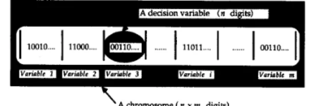
Fig. 1. Encoding decision variables as a chromosome.
I = (0, l}L X E N L E N f : I + R s : I X + I c : I2 + 1 2 m : I + I T : I’ + (0, l} Initial population Encoding of chromosomes Population size Length of Chromosome Fitness function Parent-selection operation Crossover operation Mutation operation Termination criterion There are X chromosomes in each population. The initial population of chromosomes, po, is generated randomly. The entity ai denotes the kth chromosome in the tth generation of population, pt. A chromosome, I , is encoded as a string of binary digits, 1’s and 0’s. If there are w decision variables in an optimization problem and each decision variable is encoded as an n-digit binary number, then a chromosome is a string of
L = w x n binary digits (Fig. 1) and represented as a column vector [ u k , l , . . ‘ , a k , L ] T . The term g : X + Y denotes a function g maps
x
to y wherex
EX
and y E Y . Variables Nand R are sets of integer and real numbers, respectively. The evolution process of genetic algorithm is continued (T = 0) until one of the termination criteria is met (7’ = 1).
j = 1
The index q is obtained from
1
x
q = min IC
I
V~C E ( 1 , ...
, A > , s.t. ai5
f ( a t , ).
{
k = lC . Crossover Operation
For any pair of selected chromosomes in a population p t , an associated real value, 0
5
pI
1, is generated randomly. If p is greater than the predefined crossover threshold, pc,the crossover operator is applied to this pair of chromosomes. Three different crossover strategies have been applied in this work. The first one is two-point crossover, ctptr that produces an intermediate population p f t from the population pt and is defined below in (l), where 1
5
p 1<
pz5
L. In this crossover strategy, two positions in a pair of chromosomes are selected. The pair of chromosomes are divided into three sub-chromosomes by these two points and crossed over to each other by swapping the first and third sub-chromosomes.The second crossover strategy is multi-point crossover, cmp, that produces an intermediate population pit from the population p t and is defined as (see (2) below) where 0
5
p k , pmp I 1. In this crossover strategy, more than one crossover points are selected in a pair of chromosomes. The crossover operator is performed in bit level (allele in a chromosome). That is, the process of crossover is performed bit by bit. The numbers of crossover points and crossover positions in each pair of chromosomes are selected randomly, distinctly from each other.
The third crossover strategy is uniform crossover, tun, that
produces an intermediate population ptt from the population
p t . First, a mask, a binary array with length L, is generated. L real values, 0
5
r j5
1 ( j = 1 , 2 ,. . . ,
L ) , are generated randomly. If the jth random number, r j , is greater than or equal to the predefined threshold value, pma, the value of thejth element in the binary array is set as 1. Otherwise, it is set B . Parent Selection
The parent selection operation, s, produces an intermediate population p’t = ( a y , .
. .
,a’,”) from the population p t ={
} = e m p ( { !(})
V i € ( 1 , 3 , . . . , 2 k + l , . . . , X - l ) a’tz+l) atz+l)902 IEEE TRANSACIIONS ON NEURAL NETWORKS, VOL. 5, NO. 6, NOVEMBER 1994 Before crossover ... Strmg 1 i I
I
" After crossover New String 1I
'
p, p, L (1). Two-ooint crossova Before crossover ... After crossover New Stnne 1Before crossover After Crossover
New String 1
String 1
IlllIIlIIllIll
"TW
Siring 2
II)
New String2mm
LulI"
1 P; PI, r,i L (3). Uniform -c
Fig. 2. Two-point, multi-point, and uniform crossovers.
as 0. The mask, ma, is defined as
ma = u,L_,(([1]%ifrj
L.
pma)v
([01,if rJ<
P m a ) }The uniform crossover is defined as shown in (3) below. Similar to the multi-point crossover strategy, the process of uniform crossover is performed bit by bit in a pair of chromosomes. In the uniform crossover strategy, the crossover positions are predefined in a mask. All chromosomes in a population are crossed over in the same positions. On the other hand, in the multi-point crossover strategy, each pair of chromosomes are crossed over at different points because no predefined mask is used. Three aforementioned crossover operators are shown schematically in Fig. 2.
D. Mutation Operation
For any chromosome in a population p t , an associated real value, 0
5
p5
1, is generated randomly. If p is less than the predefined mutation threshold, pm, the mutation operator is applied to this chromosome. The mutation operator simply alters one bit from 0 to 1 (or 1 to 0) in a chromosome. As the mutation operator is not guided by the fitness (objective) function, the result of mutation operator can make an instant change between two successive generations. The operator ofSecond Stace
a
First,StaeeGenetic Algoorith
The control flow of thc f m t l c a r n i n ~ "rlage "
The control flow of the second learning stage
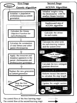
Fig. 3.
conjugate gradient neural network leaming algorithm.
A hybrid leaming algorithm using genetic algorithm with adaptive
mutation, m, produces an intermediate population p't from the population pt and is defined as:
ait
=: m(at) V i E { 1 ; . . , X ]U + f o r k E { 1 , 2 , . , . , p - l , p + 1 , . . . ! L }
U i , k for k = p where 1
5
p<
L.111. A HYBRID GENETIC/ NEURAL
NETWORK LEARNING ALGORITHM
A hybrid leaming algorithm using genetic algorithm with adaptive conjugate gradient multilayer neural networks is presented in Fig. 3. It consists of two leaming stages. The first learning stage is used to accelerate the whole leaming process by using a genetic algorithm with the feedfonvard step of the adaptive conjugate gradient neural network (ACGNN) leaming algorithm. The genetic algorithm performs global search and seeks a near-optimal initial point (weight vector) for the second stage. In this stage, each chromosome is used to encode the weights of neural network. The fitness (objective) function for the genetic algorithm is defined as the average squared system error of the corresponding neural network. Therefore, it becomes an unconstrained optimization problem: find a set of
HUNG AND ADELI: A PARALLEL G/” LEARNING ALGORITHM FOR MIMD SHARED MEMORY MACHINES
~
903
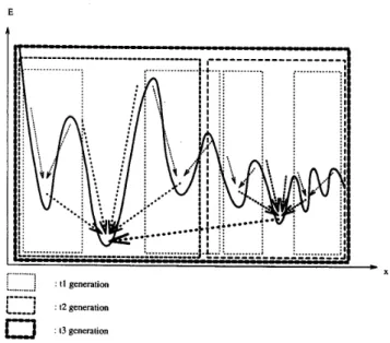
Fig. 4. Global search using genetic algorithm.
decision variables minimizing the objective function. The best fitness function value in a population is defined as the smallest value of the objective function in the current population.
The process of global search using genetic algorithm is
schematically presented in Fig. 4. Consider three consecutive generations, t l , t 2 , and t3. The chromosomes in tl generation perform local search in some discrete domain. After applying the crossover and mutation operators to the tl generation, the chromosomes with lower fitness function are selected as the parents, the chromosomes with higher fitness function are discarded, some new chromosomes are generated via the selected parent chromosomes, and the t l generation is replaced by the new population of chromosomes called t 2 generation. In the t2 generation, the chromosomes perform local search in a larger domain than t l generation and approach to some local minimums with lower fitness function values. In the t3 generation, the chromosomes with lower fitness function in the t 2 generation are selected and new chromosomes are generated that cover the whole bounded domain. In this last generation, the chromosomes perform global search in the whole bounded domain and approach to the global minimum in the domain.
After performing several iterations and meeting one of the stopping criteria, the first learning stage is terminated and the chromosome retuming the minimum objective function (the best seed) is considered as the initial weights of the neural network in the second stage. Next, the adaptive conjugate gra- dient learning algorithm performs the second learning process until the terminal condition is satisfied.
In order to reduce the memory storage requirement and increase the computational efficiency, the allele (binary digit) of each chromosomes in a population is encoded as a bit rather than an integer. In this case, the length of each chromosome is equal to the length of an integer, such as 16 bits on a SUN SPARC station. Hence, the memory storage used for each chromosome is an integer rather than a sixteen-element
X
integer array. Since we encode the chromosome as an integer, the operations of crossover and mutation can be operated using bitwise operators that are directly performed via computer hardware.
Consider a multilayer neural network with N [ i ] nodes in layer i. The learning problem is mapped from N [ 1 ] input nodes to N [ m ] output nodes and a number of N , instances are given as training examples. The total number of weights and nodes are denoted by N , and N,, respectively. For the genetic algorithm, we assume N p chromosomes are generated and operated on in each iteration. The operators and other features of the genetic algorithm are the same as those defined previously.
The first learning stage is a combination of the genetic algorithm with the feedforward process of the adaptive con- jugate gradient learning algorithm. In each iteration of this learning stage, the chromosome with the smallest value of objective function is saved as subbest-chromosome and com- pared with the one saved in the previous iteration, called best-chromosome. After the first learning stage is terminated, the best-chromosome is used as the initial weight vector for the second learning stage. In order to reduce redundant computations in this learning stage, three different stopping criteria are employed to terminate this learning process. If one of these three stopping criteria is met, the first learning stage is terminated.
The smallest value of the objective functions in a population is less than the acceptable predefined value. The fitness ratio, defined as the value of the best-chromosome’s objective function to the average value of objective functions, is greater than 0.95. If the objective function of the best-chromosome does not change in a predefined number of consecutive iterations (in this work, a value of 10 is used for this number).
904 IEEE TRANSACTIONS ON NEURAL NETWORKS, VOL. 5 , NO. 6, NOVEMBER 1994
TABLE I
THE FIRST STAGE OF THE PARALLEL HYBRID LEARNING ALGORITHM
First Learning Stage
*I
Initialize the chromosomes randomly as current generation, initialize working parameters, and set the first chromosome as the best- chromosome.
Parallel region l - e n t r y
For i = 1 to N p , do concurrently
a) Initialize sub-totalfitness to zero and subbest- chromosomes as null. b) For j = 1 to chunksize, do sequentially
a) For k = 1 to N , , do sequentially
a l ) Perform feedforward procedure of the adaptive conjugate gradient learning algorithm. a2) Calculate the objective function (system error for the neural network).
Next k
b) Calculate the sub-total- fitness by accumulating objective function of each chromosome. c) Store the best- chromosome as subbest-chromosome.
Next j
Guarded section l-entry
c) Calculate the total- fitness by accumulating sub-total- fitness.
d) Compare the sub-best-chromosome with each other and set the best subbest-chromosome as the best- chromosome. Guarded section l - e n d
Next i
Parallel region l - e n d DO
Parallel region 2-entry
e) For i = 1 to ( N p / 2 ) , do concurrently
d) Initialize sub-total- fitness to zero and subbest- chromosome as null. e) For j = 1 to chunksize, do sequentially
e l ) Select parents using roulette wheel parent selection.
e2) Apply two-point, multi-point, or uniform crossovers and mutation to the parents. e3) For
k
= 1 to N , , do sequentiallye3.1) Perform feedforward procedure of the adaptive conjugate gradient learning algorithm to parent chro- e3.2) Calculate the objective function (system error for the neural network) for parent chromosomes.
mosomes. Next k
e4) Calculate the sub-total- fitness by accumulating objective function of each chromosome. e5) Store the best- chromosome as subbest- chromosome.
Next j
Guarded section 2 - e n t r y
f) Calculate the total- fitness by accumulating sub-total- jitness.
g) Compare the subbest- chromosome to each other and set the best subbest- chromosome as the best- chromosome. Guarded section 2--end
Next
i
Parallel region 2 - e n d
f) Replace the old generation by the new generation. WHILE ('stopping criteria).
The first stage of the parallel hybrid learning algorithm is presented in Table I and shown schematically in Fig. 5.
The second learning stage is a stand-alone adaptive conju- gate gradient neural network learning algorithm. A number of
N , tasks are created and executed concurrently. The second stage of the parallel hybrid neural network learning algo-
rithm is presented in Table I1 and shown schematically in Fig. 6.
IV. APPLICATIONS
We apply the parallel hybrid geneticheural network learning algorithm developed in this research to two different domains:
HUNG AND ADELI: A PARALLEL G/” LEARNING ALGORITHM FOR MIMD SHARED MEMORY MACHINES 905
TABLE I1
THE SECOND STAGE OF THE PARALLEL HYBRID LEARNING ALGORITHM
Second Learning Stage *I
Set the best-chromosone as the initial weight vector, set up the topological structure of neural network, and set the counter cnt to zero.
DO
Parallel region-entry
a) For i = 1 to N s , do concurrently
a) Initialize subsystem-error and subdeltaweights to zero. b) For j = 1 to chunksize, do sequentially
b l ) Perform feedforward procedure of the adaptive conjugate gradient learning algorithm. b2) Calculate subsystem-error.
b3) Calculate the deltas in output layer.
b4) Calculate the deltas in hidden layers (from layer m - 1 to layer 1).
b5) Calculate the subdeltaweights in hidden layers (from layer m - 1 to layer 1). Next j .
Guarded section-ntry
c) Calculate the system error, E, by accumulating subsystem-error. d) Calculate deltas of weights by accumulating the subdelfa-weights.
Guarded section-nd
Next i.
Parallel region-nd
If cnt
2
1, calculate the new conjugate gradient direction. Perform inexact line search to calculate the step length. Update the weight vector.WHILE (“stop criteria). )
engineering design and image recognition. Three examples are presented, one in the domain of engineering design and two in the domain of image recognition.
Example I Engineering Design: This example is the selec- tion of a minimum weight steel beam from the AISC LRFD
wide-flange (W) shape database [4] for a given loading condi- tion [2], [9], [lo]. Each instance consists of five input pattems:
the member length, the unbraced length, the maximum bending moment in the member, the maximum shear force in the member, and the bending coefficient. The output pattern is the plastic modulus of the corresponding least weight member.
A four-layer feedforward neural network with two hidden layers was used to learn this problem. The numbers of nodes in the input layer, the first and second hidden layers, and the output layer are 5, 5, 3, and 1, respectively. There are 52 links in this neural network. We use ten training instances in this example. The total number of iterations for learning process is limited to 100. The working parameters for the first stage of leaming (genetic algorithm) are as follows: population size:
4000, length of decision variable: 16 bits, chromosome length: 832 (52 x 16) bits, crossover rate: 0.8, mutation rate: 0.08, and range of decision variables: -5 to 5.
Initialize a population of c h m ” e s as cumnt generahon Perfom feedforward p-s of ACGNN algorithm Calculate the fitness for each chmmosom Calculate the summahon of total fitness and store the best-chromosome
S e k t parent chromosomes and apply crossover and mutahon operators to the parent chromosomes
Perform feedforward p-s of ACGNN algorithm Calculate the fitness for each chromosome Calculate the summahon of total fitness and store the best-chromorome Generate a new generation and use it as current generation Store the best-chromosome
.
N oD ~AYes ~ ~I22gz:d
?a
ACGNNExample 2 h u g e Recognition (7 X 7 Binary h a g e S Of
Numerals): This example is recognition of seven by seven (7 x 7) binary images of the numerals (0 to 9) (Fig. 7). A three-layer neural network with one hidden layer was used to learn this problem. The numbers of nodes in the input
Fig. 5. The first learning stage of the parallel hybrid neural network learning algO*thm.
layer, the hidden layer, and the output layer are 49, 99, and 10, respectively. The total number of links in this three-layer
906 IEEE TRANSACTIONS ON NEURAL NETWORKS, VOL. 5, NO. 6, NOVEMBER 1994
lnihalize weights using the m u l t of the fint learning stage by decoding the chromsome with the smallest fitness function
Inihalize working variable Perform feedforward process, calmlate the error term for each haining instanrr. and calculate the deltar for each instance
Calculate the system error E and the summation of deltas of weights
Calculate the new
conjugate dtrwtion
Perform parailel inexact line search to find the step length Update the weight vector
Fig. 6.
learning algorithm.
The second leaming stage of the parallel hybrid neural network
neural networks is 5950. The total number of iterations for leaming process is limited to 200. There are 30 instances in the training set: ten noiseless image instances and 20 image instances with about 10% noise (5 pixels out of 49 pixels). The working parameters for the first stage of learning (genetic algorithm) are as follows: population size: 250, length of decision variable: 16 bits, chromosome length: 95 200 (5950 x 16) bits, crossover rate: 0.8, mutation rate: 0.08, range of decision variables: -1 to 1.
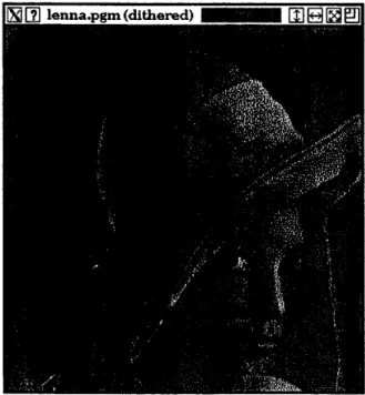
Example 3 Image Recognition (Lenna Image): This exam- ple is to recognize an 8-bit gray-scale (256 gray levels) of the Lenna image (Fig. 8). Each training instance is an eight by eight (8 x 8) square image Thus, the 384 x 384 pixel Lenna image is decomposed into 2304 training instances used to train the feedforward neural network. A flat (two-layer) neural network was used to learn this example. The number of nodes in both input and output layer is 64. The total number of links in this two-layer neural networks is 4,160. The total number of iterations for learning process is limited to 50. The working parameters for the first stage of learning (genetic algorithm) are as follows: population size: 250, length of decision variable:
16 bits, chromosome length: 66 560 (4160 x 16) bits, crossover rate: 0.9, mutation rate: 0.095, range of decision variables: - 1 to 1.
Fig. 7. Ten noiseless and 20 noisy 7 x 7 binary images of numerals (0 to 9).
V. COMPUTATION RESULTS
Fig. 8. The 8-bit gray-scale (256 levels) Lenna image.
A . Convergence History
Example 1 : The system error for this example using the adaptive conjugate gradient neural network learning algorithm and the parallel hybrid neural network algorithm are shown in Fig. 9. After 12 iterations of learning process, the first leaming
stage of the parallel hybrid neural network learning algorithm met one of the stopping criteria. The best fitness function was a value of about 0.0023. The result of the first leaming stage is used as an initial weight vector in the second learning stage.
HUNG AND ADELI: A PARALLEL GI” LEARNING ALGORITHM FOR MIMD SHARED MEMORY MACHINES 750 700 650 ~ 907 ~ -
.~
, I,
System errorAdaphve Conjugate g r d e n t neural network learmng algonthm
I 0 0 ~I...
000
L- . ~ ~ -1-- lrcrarlons
OW 2000 4000 6000 sow 10000
Fig. 9. System error for the minimum weight steel beam design.
System error E
- H y h d genehclneural network
learrung algorithm
--____. Adaphve Conjugate grahent neural network leanung alpnthm
I I I10 I 090 1 ” 080
:
I-
i l
I
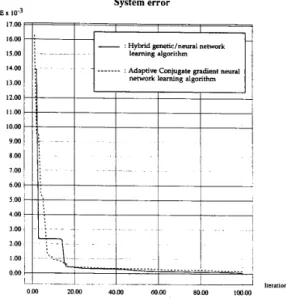
om 0 IO OW 000 2000 4000 6000 80W 10000 Iterations Fig. 10. (0 to 9).System error for the 7 x 7 binary image recognition of numerals
After a total of 100 iterations of the learning process, the system error in the parallel hybrid neural network learning algorithm converges to a value 6.5 x The stand-alone adaptive conjugate gradient neural network learning algorithm converges to 1.84 x after 100 iterations of the learning process.
ExumpZe2: The system error for this example using the adaptive conjugate gradient neural network learning algorithm and the parallel hybrid neural network learning algorithm are shown in Fig. 10. After 18 iterations, the first learning stage of the parallel hybrid neural network learning algorithm met one of the stopping criteria. The best fitness function has a value of about 0.3. The result of the first learning stage is used as
System error E
Adaphve Conjugate gradient neural network leanung algonthm
no0 moo 2000 3000 ~ o o o ,000
System error for the Lenna image recognition problem Fig. 11.
an initial weight vector for the second learning stage. After 12 more iterations, the system error in the parallel hybrid neural network learning algorithm converges to a value of less than 0.001 and the algorithm achieves 100% recognition of all the 30 training instances.
After the same number of iterations, the stand-alone adap- tive conjugate gradient neural network learning algorithm converges to a value of 0.17 and recognize about 63% (19 out of 30) of the training set.
ExampZe3: The system error for this example using the adaptive conjugate gradient neural network learning algorithm and the parallel hybrid neural network learning algorithm are shown in Fig. 11. After eight iterations of learning process, the first learning stage of the parallel hybrid neural network learning algorithm met one of the stopping criteria. The best fitness function was a value of about 4.4. The result of the first learning stage is used as an initial weight vector for the second learning stage. After 42 more iterations, the system error in the parallel hybrid neural network learning algorithm converges to a value of 0.10. The stand-alone adaptive conjugate gradient neural network learning algorithm converges to a value of 0.15 after 50 iterations.
B . Speedup
The speedup is measured by using an expert system tool, called utexpert. A neural network with 52 links is used in ex- ample 1. In the first learning stage of the parallel hybrid neural network learning algorithm, 4000 chromosomes are operated on in each learning iteration. That is, 4000 tasks are created and performed concurrently in this stage. Each concurrent task performs the computation of a stand-alone neural network with 10 training instances. The overall speedup achieved by the parallel hybrid neural network learning algorithm for example 1 is dominated by the first learning stage. As the genetic algorithm is an intrinsically parallel algorithm, the maximum
908 IEEE TRANSACTIONS ON NEURAL NETWORKS, VOL. 5, NO. 6 , NOVEMBER 1994 10 8 3 6 -a
k
VI 4 2 0 I.. < ‘ / _ . < I I- t I I I I I I I 0 2 4 6 8 I I I I I I I I1
No of processors Fig. 12.network leaming algorithm without vectorization.
Speedup for examples 1-3 using the parallel hybrid genetic/neural
speedup of example 1 due to microtasking is about 7.9 using eight processors of the Cray Y-MP8/864 supercomputer (Fig. 12). A maximum average speedup of about 9 is achieved when microtasking is combined with vectorization using eight processors of the Cray machine (Fig. 13). In this example, the value of speedup due to a combination of microtasking with vectorization is not high because the loop performed by vector operation is short.
A very large neural network with 5950 links is used in example 2. Two hundred fifty (250) chromosomes are operated on in each learning iteration. That is, 250 tasks are created and performed concurrently in this learning stage. Each concurrent task performs the computation of a stand-alone neural network with 30 training instances. The overall speedup achieved by the parallel hybrid neural network leaming algorithm for example 2 is also dominated by the first learning stage. The maximum speedup due to microtasking is about 7.4 using eight processors of the Cray Y-MP8/864 supercomputer (Fig. 12). A maximum average speedup of about 17.6 is achieved due to a combination of microtasking with vectorization (Fig. 13).
A very large neural network with 4160 links is used in ex-
ample 3 with 2304 training instances. Two hundred fifty (250)
chromosomes are operated on in each learning iteration. The maximum speedup due to microtasking is about 7.3 using eight processors of the Cray Y-MP8/864 supercomputer (Fig. 12).
A maximum average speedup of about 33 is achieved when microtasking is combined with vectorization (Fig. 13).
VI. FINAL REMARKS
We have presented a parallel hybrid neural network learning algorithm by integrating genetic algorithm with an adaptive
35 30 25
9
20 15 10 5 0 0 2 4 6 8 No. of processorsSpeedup for examples 1-3 using the parallel hybrid geneticheural Fig. 13.
network leaming algorithm with vectorization.
conjugate gradient neural network learning algorithm. Follow- ing observations are made and conclusions drawn:
The results of neural network learning are sensitive to the initial value of the weight vector. In this work, a genetic algorithm is employed to perform global search and to seek a good starting weight vector for the subsequent neural network learning algorithm. The result is an improvement in the convergence speed of the algorithm.
The problem of entrapment in a local minimum is encountered in gradient-based neural network learning algorithms. In the hybrid learning algorithm presented in this paper, this problem is circumvented by using a genetic algorithm which is guided by the fitness function of a population rather than gradient direction. After several iterations of the global search, the first leaming stage retums a near-global optimum point that is used as the initial weight vector for the second leaming stage.
A large-scale multilayer neural network requires sub- stantial computing processing time in order to converge to an acceptably small system error value. By developing efficient parallel learning algorithms on multiprocessor computers we can increase the computational speedup by an order of magnitude.
REFERENCES
[ l ] H. Adeli and C. Yeh, “Perceptron leaming in engineering design,” Micmcomp. Civil Eng., vol. 4, no. 4, pp. 247-256, 1989.
[2] H. Adeli and C. Yeh, “Neural network leaming in engineering design,” in Proc. Znr. Neural Ner. Con$, Paris, France, July 9-13,1990. pp. 412-415.
131 H. Adeli and N.-T. Cheng, “Integrated genetic algorithm for optimiza- tion of space structures,” J . Aerospace Eng., ASCE, vol. 6, no. 4, pp. 315-328, 1993.
HUNG AND ADELI: A PARALLEL G/” LEARNING ALGORITHM FOR MIMD SHARED MEMORY MACHINES 909
[4] Manual of Steel Construction, Load and Resistance Factor Design. Chicago, IL: American Institute of Steel Construction, 1986. [5] R. K. Belew, J. McInemey, and N. N. Schraudolph, “Evolving networks:
Using the genetic algorithm with connectionist learning,” Computer Science and Engineering Tech. Rep. CS90-174, Univ. of California at San Diego, 1990.
[6] L. Davis, ed., Handbook of Genetic Algorithms. New York: Van Nostrand Reinhold, 1991.
[7] D. E. Goldberg, Genetic Algorithms in Search, Optimization, and Ma- chine Learning. Reading, MA: Addison-Wesley, 1989.
[8] F. Hoffmeister and T. Back, “Genetic algorithms and evolution strategies-Similarities and differences,” in Parallel Problem Solving from Nature H.-P. Schwefel and R. M m e r , eds. Berlin, Germany:
Springer-Verlag, 1991, pp. 455-469.
[9] S. L. Hung and H. Adeli, “Multi-layer perceptron learning for design problem solving,” in Proc. Int. Neural Net. Conf.. Espoo, Finland, July 24-28, 1991, pp. 1225-1228.
[IO] S. L. Hung and H. Adeli, “A model of perceptron learning with a hidden layer for engineering design,” Neurocomputing, vol. 3, pp. 3-14, 1991.
[I 11 S. L. Hung and H. Adeli, “A hybrid learning algorithm for distributed memory multicomputers,” Heuristics-The J. Knowledge Eng., vol. 4,
’ no. 4, pp. 58-68, 1991.
[12] S. L. Hung and H. Adeli, “Parallel backpropagation learning algorithms on Cray Y-MP8/864 supercomputer,” Neurocomputing, vol. 5, pp. [13] D. J. Montana and L. Davis, “Training feedfonvard networks using genetic algorithms,” in Proc. Int. Joint Conf. Artificial Intell., San Mateo, [14] D. E. Rumelhart, G. E. Hinton, and R. J. Williams, “Learning intemal representation by error propagation,” in Parallel Distributed Processing, D. E. Rumelhart, et al., ed. Cambridge, MA: MIT Press, 1986, pp. 318-362.
287-302, 1993.
CA, 1989, pp. 762-767.
S. L. Hung received the B.S. degree from the National Chiao Tung University, Taiwan in 1982, and the M.S. and Ph.D. degrees from The Ohio State University in 1990 and 1992, respectively.
He has published 14 papers in the areas of neural networks, genetic algorithms, parallel processing, fuzzy systems, and database management. He is currently an Associate Professor at the National Chiao Tung University.
Hojjat Adeli received the Ph.D. degree from Stan- ford University in 1976.
Currently, he is a Professor of Engineering and Member of the Center for Cognitive Science at The Ohio State University. A contributor to 40 research and scientific joumals, he has authored 260
research and scientific publications, including four books in various fields of computer science and engineering. He has also edited 10 books, including Knowledge Engineering, Volume I-Fundamentals and Knowledge Engineering, Volume 2 4 p p l i c a - tions (McGraw-Hill, 1990); and Supercomputing in Engineering Analysis and Parallel Processing in Computational Mechanics, (Marcel Dekker, 1992).
Dr. Adeli was the Editor-in-Chief of Heuristics-The Journal of Knowledge Engineering during 1991-1993. He is the Founder and Editor-in-Chief of the joumal Integrated Computer-Aided Engineering. He has been an organizer or member of advisoIy boards of over 25 national and international conferences and a contributor to over 80 other conferences held in 24 different countries. He was a Keynote and Plenary Lecturer at computing conferences held in Italy (1989), Mexico (1989), Japan (1991), China (1992), Canada (1992), U.S. (1993), Germany (1993), Morocco (1994), and Singapore (1994). He has received numerous academic, research, and leadership awards, honors, and recognitions. His recent awards include The Ohio State University College of Engineering 1990 Research Award in Recognition of Outstanding Research Accomplishments, and the Lichtenstein Memorial Award for Faculty Excellence.