On formulation of a transition matrix for poroelastic medium and
application to analysis of scattering problem
Chau-Shioung Yeh, Tsung- Jen Teng, and Po-Jen Shih
ABSTRACT
Based on the approach of Pao (1978) for elastic medium, we propose a set of the basis functions and an associated relationship of the material properties of the dilatational wave in the poroelastic medium. A transition matrix, which relates the coefficients of scattered waves to those of incident waves, is then derived through the application of Betti’s third identity and the associated orthogonality conditions for the poroelastic medium. To illustrate the application, we consider a simple case of the scattering problem of a spherical inclusion, either elastic or poroelastic, embedded within the surrounding poroelastic medium subjected to an incident plane compressional wave.
I. INTRODUCTION
In a poroelastic medium, Biot (1956a,b) predicted firstly the existence of an additional propagating dilatational wave and then Plona (1980,1982) reported experimental observation of this wave. Berryman (1980) analyzed Plona’s data and then confirmed Biot’s theory. Since then the wave propagation in such a medium has become an attractive topic for physical fields.
Deresiewicz and Skalak (1963) derived a set of boundary conditions that are sufficient to guarantee a unique solution to Biot’s equations when an interface separates a poroelastic medium from the others. Many studies have applied these conditions to the reflection and transmission of incident waves at a planar interface separating infinite half-spaces. While the reflection of a wave from a planar interface is essentially a scattering phenomenon, little work has been done on the scattering from three-dimensional-bounded inclusion embedded within a poroelastic medium. Berryman (1985) derived the multipole expansion of a field scattered by a spherical inhomogeneity within poroelastic media. Zimmerman and Stern (1993a,b) also treated the scattering of a plane compressional wave by a spherical inclusion embedded in an infinite poroelastic medium. However, their solutions are obtained only for the spherical inclusion composed of elastic solid, fixed rigid, or fluid. Morochnik, et al (1996) proposed an approximate method based on the definition of equivalent-viscoelastic materials to study the scattering of plane dilatational waves by a spherical poroelastic inhomogeneity. All the preceding studies are only for spherical inclusion. The transition matrix first proposed by Waterman (1976) is a convincing method to treat an elastic obstacle of arbitrary shape. Kargl and Lim (1993) developed the transition matrix for poroelastic medium. They followed Pao’s approach for elastic medium to prove the orthogonality conditions of the basis functions for the
poroelastic medium using Betti’s identity and the far-field asymptotic formulations. Then Lim (1994) combined their previous paper (Kargl and Lim, 1993) with a generalization of existing acoustic wave-guide solutions to solve a more complicated problem: an obstacle buried in a plane porous medium. It should be noted that Kargl and Lim (1993) did not prove the relationships between two dilatational waves in the third orthogonal condition (regular-singular relationship) throughout; moreover, the far-field asymptotic formulation (which with S∞ ) or the Wronskian formula is inadequate to prove the orthogonality conditions, we have to consider other conditions from the material properties as well (i.e. Eqs.(A.8) and (A.14)).
In this paper, we adopt Pao’s (1978) approach to develop the transition matrix for a poroelastic medium. We reduce the coupled equations of motion to two parts: the dilatational part and the rotational one. The latter part is easily shown to satisfy the vector Helmholtz equation with a complex shear wave number, and the associated basis functions are expressed in terms of the vector spherical wave functions. On the other hand, the decomposition of the dilatational waves, the fast and the slow ones, are governed by two scalar Helmholtz equations. In order to obtain the independent and orthogonal sets of these two basis functions, we reconstruct these functions by normalizing with characteristic vectors elaborately. Although Halpern and Christiano (1986) have reported the normalizing procedure by the numerical method, the result has not been expressed in an analytical form in their study. In our formulation, we present the basis functions in an analytical form and preserve their indispensable features for the orthogonality relationships as well. Instead of the asymptotic method, we apply the Wronskian formula to prove the orthogonality conditions. To illustrate the application of the transition matrix formulation in our study, we present the solutions for the scattering of the incident plane waves by a spherical inclusion, either
poroelastic or elastic, embedded within a poroelastic medium.
The numerical results for the elastic spherical inclusion are presented such that the comparison can be made with those obtained by Zimmerman and Stern (1993a). We also present the results of the amplitude of radial displacement and the normal traction at the surface of the inclusion. Some illustrative numerical results show that the regions near the interface have stronger interference which is caused by the coupling effects of the dilatational and rotational waves. The difference between the elastic and poroelastic inclusions shows that the amplitude of normal traction for elastic case has more obvious patterns with larger values.
II. THE BASIS FUNCTIONS AND THE ORTHOGONALITY CONDITIONS A. Betti’s third identity for the poroelasticity
Let u( )A and u( )B be two admissible displacement fields in a poroelastic medium, and σ and ( )A σ be the corresponding stress tensors. The superscripts (A) ( )B and (B) denote two different fields in the controlled system. At a surface with a unit outward normal vector n , the traction vector is given by
( )
( )=n σ u⋅ .
t u (1)
For a poroelastic material with material constants λc, μ , α , and M (Biot, 1962,1963), the stress-strain relations are
2 ( ) , . ij ij ij c f e e M p Me M σ μ δ λ α ς α ς = + − = − + (2)
The physical quantities in the preceding equations are defined as follows: u is the displacement vector of solid with components u , i eij = ∂ ∂ + ∂12( ui xj uj ∂xi) ,
e= ∇ ⋅ u, ς = −∇ ⋅ w , w is the displacement vector of fluid relative to solid with components w , i pf is the fluid pressure in the pores, σij is the total stress in the medium, δij denotes Kronecker symbol. For the harmonic wave with circular frequency, ω , the time factor, exp( )i tω , is suppressed in all the following expressions. Then the equations of motion are reduced to
2 2 , 2 2 , , , ji j i f i f i f i m i u w p u w σ ρω ρ ω ρ ω ρ ω = − − = + (3)
where ρ is the mass density of the mixed medium, and ρf is that of the fluid. * *
m m ib
ρ = − ω represents the complex (frequency dependent) mass density of viscous fluid in a rigid framed medium where m* and b* denote the inertia parameter and the viscous dissipation parameter, respectively.
Applying Eq. (3) for a controlled volume V bounded by a closed surface Sv, the following identity can be obtained easily,
( ) ( ) ( ) ( ) ( ) ( ) ( ) ( ) , , , , {[ B A B ( A )] [ A B A ( B )]} 0 . i ji j i f i i ji j i f i V u σ +w −p − u σ +w −p dV =
∫∫∫
(4)On the basis of the assumption that ( )A i
u , ( )B i
u , and their first and second derivatives are continuous inside the volume V , we obtain the following equation by applying the divergence theorem,
( ) ( ) ( ) ( ) ( ) ( ) ( ) ( ) , , , , ( ) ( ) ( ) ( ) ( ) ( ) ( ) ( ) ( ) ( ) ( ) ( ) ( ) ( ) ( ) ( {[ ( )] [ ( )]} {[ ( )] [( ) ( )]} {[ ] [ V B A B A A B A B i ji j i f i i ji j i f i V A B A B B A B A ji i j f i i ji i j f i i V S A B A B B A B A ji ij f ji ij f V u w p u w p dV u n p w n u n p w n dS e p e p σ σ σ σ σ ς σ ς + − − + − = + − − + − − + − +
∫∫∫
∫∫
∫∫∫
w
)]}dV . (5)With the aid of Eqs. (2) and (4), Eq. (5) can be reduced to a surface integral referred to as the poroelastic reciprocal theorem,
( ) ( ) ( ) ( ) ( ) ( ) ( ) ( ) [ ] [ ] 0 . V A B A B B A B A f f V S ⋅ − p ⋅ − ⋅ −p ⋅ dS =
∫∫
t u n w t u n ww
(6)Furthermore, the closed surface SV may be deformed into another closed surface without encompassing any discontinuities during the deformation.
B. Decomposition and normalization of equations of motion
Substitution of Eq. (2) into (3) yields the coupled governing equations:
2 2 2 2 2 ( ) , ( ) . c f f m e M Me M μ λ μ α ς ρω ρ ω α ς ρ ω ρ ω ∇ + + ∇ − ∇ = − − ∇ − + = + u u w u w (7)
The displacements u and w are decomposed into two scalar potentials ϕ ϕs, f, one vector potential ψs, and one factor μ3,
3 , ( ) , 0 . s f s ϕ ϕ μ = ∇ + ∇ × = ∇ + ∇ × ∇ ⋅ = s s u ψ w ψ ψ (8)
The subscript s and f represent the solid and the relative fluid, respectively. Substitution of Eq. (8) into the coupled equations (7) yields two parts: the rotational part and the dilatational one. The rotational part is written as,
2 2 3 0, , s f m k μ ρ ρ ∇ + = = − s s ψ ψ (9) where [ ( 2 )] s f m
k =ω ρ− ρ ρ μ is the rotational wave number. The dilatational part is written in a matrix form,
2 2 2 ( 2 ) 0 . 0 f s s c f m f f M M M ρ ρ ϕ ϕ λ μ α ω ρ ρ ϕ ϕ α ⎧∇ ⎫ ⎧ ⎫ + ⎡ ⎤ ⎡ ⎤⎪ ⎪+ ⎪ ⎪=⎧ ⎫ ⎨ ⎬ ⎢ ⎥⎨ ⎬ ⎨ ⎬ ⎢ ⎥ ∇ ⎪ ⎪ ⎪ ⎪ ⎣ ⎦⎩ ⎭ ⎣ ⎦⎩ ⎭ ⎩ ⎭ (10)
Two characteristic values in Eq. (10) are obtained as follows,
2 2 (k ω) =(B± B −4AC) 2 ,A (11) where 2 2 [( 2 ) ] , [ ( 2 ) ( 2 )] , [ ] . c m c f m f A M M B M C λ μ α ρ λ μ ρ α ρ ρ ρ ρ = + − = + + − = − (12)
Two corresponding characteristic vectors associated with the characteristic values in Eq. (11) are obtained as shown below,
1, 1 2 , 1 and 1, 2 1, 2 , T T T T d c d a μ = − μ = (13) where 2 ( ) , ( 2 ) , ( 2 ) , 4 , m f m c f c a M b M c M d b b ac α ρ ρ ρ ρ λ μ α ρ ρ λ μ = − = − + = − + = − + (14) and 1 2 2 , 2 . d c d a μ μ = − = (15)
After certain elaborative manipulations, we obtain a set of characteristic vectors, 1 2 1 . 1 μ μ ⎡ ⎤ = ⎢ ⎥ ⎣ ⎦ Φ (16)
Then Eq. (10) can be normalized to the diagonal matrix form: * 2 * 1 2 1 * 2 * 2 2 0 0 ( 2 ) 0 , 0 0 0 c m M ϕ ρ ϕ λ μ ω ϕ ρ ϕ ⎡ ⎤ ⎧ ⎫ ⎡ + ⎤ ∇ ⎧ ⎫ ⎧ ⎫ + = ⎨ ⎬ ⎢ ⎥⎨ ⎬ ⎨ ⎬ ⎢ ⎥ ∇ ⎩ ⎭ ⎩ ⎭ ⎣ ⎦ ⎩ ⎭ ⎣ ⎦ (17) where 1 2 1 2 2 1 1 2 1 ( ) , 1 1 ( ) , 1 s f f s ϕ μ ϕ ϕ μ μ ϕ μ ϕ ϕ μ μ = − − = − − (18) and * 2 1 1 * 2 2 2 * 2 1 1 * 2 2 2 ( 2 ) ( 2 ) 2 , ( 2 ) 2 , 2 , 2 . c c c f m m f m M M M M M λ μ λ μ μ α μ λ μ α μ μ ρ ρμ ρ μ ρ ρ ρ ρ μ ρ μ + = + + + = + + + = + + = + + (19)
The details in the derivation of Eq. (17) are discussed in Appendix A. From Eq. (17), we readily obtain two uncoupled scalar Helmholtz equations,
2 2 1 1 1 2 2 2 2 2 0 , 0 , p p k k ϕ ϕ ϕ ϕ ∇ + = ∇ + = (20) where 2 2 * * 1 (kp ω )≡ρ (2μ λ+ c) and 2 2 * * 2
(kp ω )=ρm M . k and p1 k denote the p2 fast and slow dilatational wave numbers, respectively.
C. The basis functions in the spherical coordinates
For waves in a three-dimensional poroelastic medium, the total motions may be decomposed into four parts: L1, L2, M , and N . L and 1 L represent the 2
dilatational motions propagating with speeds c and p1 c , and wave numbers p2
1 1
p p
k =ω c and kp2 =ω cp2; M and N are the rotational ones propagating with speed c and wave number s ks =ω cs . The three wave speeds are given by
* * 1 (2 ) p c c = μ λ+ ρ , * * 2 p m c = M ρ , and ( 2 ) s f m c = μ ρ ρ ρ− , respectively. In spherical coordinates( , , )Rθ φ , similar to the expression for elastic media (Morse and Feshbach,1953), we propose four wave functions for the vector displacements of solid for a poroelastic medium as follows:
(1) 1 (2) 1 1 (2) 1 1 (2) 2 1/ 2 1 1 1 [ ( ) ( , )] ( ) { ( ) ( ) } , mn mn n p mn p p n p n p mn mn p p h k R Y k k h k R h k R n n k k R σ σ σ σ σ μ θ φ μ = = ∇ ′ = + + u L A B (21) (2) (2) 2 2 (2) 2 (2) 2 1/ 2 2 2 2 1 [ ( ) ( , )] ( ) { ( ) ( ) } , mn mn n p mn p p n p n p mn mn p p h k R Y k k h k R h k R n n k k R σ σ σ σ σ θ φ = = ∇ ′ = + + u L A B (22) (3) (2) 2 1/ 2 (2) [ ( ) ( , ) ] ( ) ( ) , mn mn n s mn n s mn h k R Y R n n h k R σ σ σ σ θ φ = = ∇ × = + R u M e C (23) (4) (2) (2) 2 2 1/ 2 1 ( ) [ ( )] ( )( ) ( ) , mn mn mn s n s s n s mn mn s s k h k R k R h k R n n n n k R k R σ σ σ σ σ = = ∇ × ′ = + + + u N M A B (24) where 2 ( 2 ) p c
k ≡ ω ρ λ + μ is a convenient common wave number used to make the basis function dimensionless. The symbol σmn is an abbreviation for three integers: σ from 1(even) to 2 (odd), m from 0 to n, and n from 0 to ∞ . The function (2)( )
n
h x is the second kind of the spherical Hankel function, and (2) (2) (2)
[xhn ( )]x ′ =xhn ′( )x +hn ( )x and (2)( ) (2)( )
n n
harmonics ( , )Yσmn θ φ consists of an even part (σ =1) and an odd one (σ =2), 1 2 ( , ) (cos )cos , ( , ) (cos )sin , m mn n m mn n Y P m Y P m θ φ θ φ θ φ θ φ = = (25) where m(cos ) n
P θ are the associated Legendre polynomials, m=0, 1, ," n and 0, 1, ,
n= " ∞. The three mutually perpendicular vectors Aσmn, Bσmn, and Cσmnare related to the three unit vector e , R e , and θ e in the spherical coordinates, φ
2 1/ 2 2 1/ 2 , ( ) [ ] , sin ( ) [ ] . sin mn R mn mn mn mn mn Y n n Y n n Y σ σ σ θ φ σ σ θ φ σ θ θ φ θ φ θ − − = ∂ ∂ = + + ∂ ∂ ∂ ∂ = + − ∂ ∂ A e B e e C e e (26)
According to Eqs. (8) and (18), the vector operators of relative displacements of fluid are obtained as follows,
(2) 1 1 (1) (2) 2 1/ 2 1 1 (2) 2 2 2 (2) (2) 2 1/ 2 2 2 (3) 2 1/ 2 (2) 3 (2) (4) 2 3 ( ) ( ) [ ( ) ( ) ] , ( ) ( ) [ ( ) ( ) ] , ( ) [( ) ( ) ] , ( ) ( ) [( )( p n p mn n p mn mn p p p n p mn n p mn mn p p mn n s mn n s mn k h k R h k R n n k k R k h k R h k R n n k k R n n h k R h k R n n σ σ σ σ σ σ σ σ σ μ μ μ ′ = + + ′ = + + = + = + w u A B w u A B w u C w u (2) 2 1/ 2 [ ( )] ) ( ) ( s n s ) ] . mn mn s s k R h k R n n k R σ k R σ ′ + + A B (27)
Whereas according to the constitutive relation Eq. (2), the scalar operators of fluid pressures are shown below,
2 1 (1) (2) 1 1 2 2 (2) (2) 2 2 (3) (4) ( ) ( 1) ( ) , ( ) ( ) ( ) , ( ) 0 , ( ) 0 . p f mn n p mn p p f mn n p mn p f mn f mn k p M h k R Y k k p M h k R Y k p p σ σ σ σ σ σ αμ α μ = + = + = = u u u u (28)
The vector operators for the tractions at a surface with a unit outward normal n can be calculated from Eq. (2), and are shown as follows,
(1) 1 1 1 1 (2) 2 2 2 2 (3) (4) ( ) ( / )( ) ( ) , ( ) ( )( ) ( ) , ( ) ( ) , ( ) ( ) . mn c mn mn mn mn c mn mn mn mn mn mn mn mn mn M M σ σ σ σ σ σ σ σ σ σ σ σ σ σ λ α μ μ λ α μ μ μ μ = + ∇ ⋅ + ⋅ ∇ + ∇ = + ∇ ⋅ + ⋅ ∇ + ∇ = ⋅ ∇ + ∇ = ⋅ ∇ + ∇ t u L n n L L t u L n n L L t u n M M t u n N N (29)
If we consider a special case of a spherical surface n e , the four traction operators = R are reduced to the following simpler forms,
2 2 1 1 (1) (2) (2) 1 1 1 1 2 1 1 (2) (2) 1 1 1 2 (2) (2) 1 1 2 1/ 2 1 1 2 1 ( ) { ( ) ( ) [ 2 ( ) 4 2 ( ) ( ) ( )]} ( ) ( ) 2 ( ) [ ] , p p r mn c n p n p p p p n p n p mn p p p n p n p mn p p k k M h k R h k R k k k n n h k R h k R k R k R k h k R h k R n n k R k R σ σ σ λ μ α μ μ μ μ μ μ = − + + − + ′ + − ′ + + − t u A B (30) 2 2 2 2 (2) (2) (2) 2 2 2 2 2 (2) (2) 2 2 2 (2) (2) 2 2 1/ 2 2 2 2 2 ( ) { ( ) ( ) [ 2 ( ) 4 2( ) ( ) ( )]} ( ) ( ) 2 ( ) [ ] , p p r mn c n p n p p p p n p n p mn p p p n p n p mn p p k k M h k R h k R k k k n n h k R h k R k R k R k h k R h k R n n k R k R σ σ σ λ α μ μ μ = − + + − + ′ + − ′ + + − t u A B (31) (2) (3) (2) ( ) 2 1/ 2 ( ) [ ( ) ]( ) , r n s mn s n s mn h k R k h k R n n R σ =μ ′ − + σ t u C (32) (2) (4) 2 2 (2) (2) 2 2 1/ 2 2 ( ) ( ) 2 { ( )[ ] ( ) ( ) ( ) [( 1 ) ] ( ) }. 2 ( ) r n s mn s mn s s n s n s mn s s h k R k n n k R k R h k R h k R n n n n k R k R σ σ σ μ ′ = + ′ + + − − − + t u A B (33)
D. Orthogonality conditions of the spherical basis functions
orthogonal relations (Morse and Feshbach, 1953), 0, 0, 0, mn mn mn mn mn mn σ σ σ σ σ σ ⋅ = ⋅ = ⋅ = A B A C B C (34)
and integrations over a spherical surface yield the following equations, 2 0 0 2 0 0 2 0 0 sin (1 ) , sin (1 ) , sin (1 ) . mn m n mn mm nn mn m n mn mm nn mn m n mn mm nn d d d d d d π π σ σ σσ π π σ σ σσ π π σ σ σσ θ θ φ γ δ δ δ θ θ φ γ δ δ δ θ θ φ γ δ δ δ ′ ′ ′ ′ ′ ′ ′ ′ ′ ′ ′ ′ ′ ′ ′ ′ ′ ′ ⋅ = ⋅ = ⋅ =
∫ ∫
∫ ∫
∫ ∫
A A B B C C (35)The normalization constant is defined as below,
(2 1)( )! 4 ( )!,
mn m n n m n m
γ =ε + − π + (36)
where 1εm= when m=0, and εm = when 2 m>0.
For the wave fields which are regular in the region enclosing the origin of the coordinate system, we use four regular basis functions ˆ( )
mn α σ
u (α =1, 2, 3, or 4) which are obtained from ( )
mn α σ
u by replacing the spherical Hankel function (2) n
h , in L1 mnσ ,
2 mnσ
L , Mσmn, and Nσmn, with the spherical Bessel function j . n
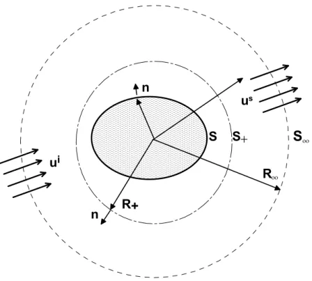
Considering an infinite region divided by a surface S of an arbitrary shape as shown in Fig. 1, we add an artificial spherical surface S+ exterior to S with radius R+. Let V in Eq. (5) be the region inside S+ first, and then let set (A) be one of a regular set and (B) be another regular set inside the region S+. Thus Eq. (6) reduces to a special case referred to as the first orthogonality condition,
( ) ( ) ( ) ( ) ( ) ( ) ( ) ( ) { ( ) ( ) ) ( ) ˆ ) ( ) } ˆ ˆ ( 0 ˆ ˆ (ˆ ˆ , ˆ mn m n m n mn mn m n S m f f n mn p dS p α β β α α β σ σ σ σ σ σ β α σ σ ′ ′ ′ ′ ′ ′ ′ ′ ′ + ′ ′ ′ ⋅ − ⋅ − ⋅ + ⋅ =
∫∫
t t u u n w n w u u u u u uw
(37)where ,α β =1,2,3, or 4. Next, let set (A) be one of a singular set and (B) be another singular one. Choose control volume to be the region bounded internally by S and
externally by S∞. Since all ( ) mn α σ
u are regular outside the region S+, we can obtain the second orthogonality condition,
( ) ( ) ( ) ( ) ( ) ( ) ( ) ( ) ( ){ ( ) ( ) ( ) ( ) ( ) ( ) } 0 . mn m n m n mn S S f mn m n f m n mn p p dS α β β α σ σ σ σ α β β α σ σ σ σ ∞ + ′ ′ ′ ′ ′ ′ ′ ′ ′ ′ ′ ′ − ⋅ − ⋅ − ⋅ + ⋅ =
∫∫ ∫∫
u u t t u n w u w u u n u u (38)The minus sign of the second integral is used because the outer normal at S+ in this case is −e . Through the zero value of Wronskian formula in Eq. (B.13) (i.e. both are R Bessel functions) and the relationship of material properties in Eqs. (A.8) and (A.14), we can prove the integrals on both surfaces S∞ and S+vanish. Finally, let set (A) be one of a regular set and (B) be a singular one outside the surface S+ and inside the surface S∞ .Through Eq. (35) and the application of the Wronskian formula (Abramowitz and Stegun, 1964), we obtain the third orthogonality condition,
( ) ( ) ( ) ( ) ( ) ( ) ( ) ( ) ( ) { ( ) ( ) ( ) (ˆ ) ˆ ( ˆ ˆ ) ( ) } ( ) , mn m n m n mn f mn m n S f m n mn s mn mm nn p p dS i k D α β β α α β σ σ σ σ σ σ β α α σ σ μ σ δ δ δ δσσ αβ ′ ′ ′ ′ ′ ′ ′ ′ ′ + ′ ′ ′ ′ ′ ′ ⋅ − ⋅ − ⋅ + ⋅ = −
∫∫
t u u t u u u n w u u u n w (39) where ( ) ( ) 4 ( )! [ (2 1)( )!] , 0 , if odd, and 0 , m mn n m n n m D m α α σ γ π ε σ ⋅ + ⋅ + − ⎧ = ⎨ = = ⎩ (40) and * 2 1 * 2 ( ) 2 2 ( 2 ) ( ) if 1 , ( ) if 2 , if 3 ,or 4 . c s p p s p p k k k M k k k n n α λ μ μ α γ μ α α ⎧ + = ⎪⎪ =⎨ = ⎪ + = ⎪⎩ (41)Eqs. (37), (38), and (39) are the desired orthogonality conditions among the basis functions that are the key step in the derivation of the transition matrix. In particular, the derivation of Eq. (39) is different from that obtained by Kargl and Lim (1993) (shown in Appendix B). Notice that the surface integrals in Eqs. (37)-(39) are
independent of radius R+. These invariant properties imply a conservation law and mean that the shape of S+ may be deformed to S, and the surface integral over S+ can be replaced with the one over S. The details of the derivation of Eqs. (37)-(39) are discussed in Appendix B.
III. THE TRANSITION MATRIX FOR AN INCLUSION
A. Series expansions of the incident, refracted, and scattered waves
Let a region inside S as shown in Fig. 1 be filled with a material different from that of the surrounding medium, and all material constants inside S are designated by a subscript (0): λc(0),μ α(0), (0), and M(0). An incident wave ui( )R impinging on the inclusion is refracted into the inclusion with the displacementu−( )R and scattered into the surrounding medium as us( )R . Each of these three kinds of waves can be represented by a series representation of the basis functions within a specific region,
4 ( ) ( ) 1 ˆ ( ) , i m n m n m n R aσβ σβ σ′ ′ ′ =β ′ ′ ′ ′ ′ ′ =
∑ ∑
u u (42) 4 ( ) ( ) 1 ( ) , s m n m n m n R cσβ σβ σ′ ′ ′ =β ′ ′ ′ ′ ′ ′ =∑ ∑
u u (43) 4 ( ) ( ) (0) 1 ˆ ( ) m n m n . m n f R β β σ σ σ β ′ ′ ′ ′ ′ ′ ′ ′ = − =∑ ∑
u u (44) The symbol m n σ ′ ′ ′∑
is an abbreviation for three summations over the indexes. The
quantities ( ) m n
aσβ′ ′ ′, cσ( )β′ ′ ′m n , and fσ( )′ ′ ′βm n denote the incident, scattered, and refracted coefficients, respectively. The incident wave in Eq. (42) is uniformly convergent for
R R< ∞. The basis functions for us( )R are regular outside and at the interface of the inclusion. Similarly, the series for u−( )R is uniformly convergent inside and at the
interface of the inclusion. The total displacement fields in the exterior region can be represented by the series in Eqs. (42) and (43),
4 4 ( ) ( ) ( ) ( ) 1 1 ˆ ( ) ( ) . i s m n m n m n m n m n m n R R aσβ σβ cσβ σβ σ′ ′ ′β= ′ ′ ′ ′ ′ ′ σ′ ′ ′β= ′ ′ ′ ′ ′ ′ = + =
∑ ∑
+∑ ∑
u u u u u (45)Since both series are uniformly convergent, we can apply the associated operators t ,
w, and pf to Eq. (45), such as the following,
4 4 ( ) ( ) ( ) ( ) 1 1 4 4 ( ) ( ) ( ) ( ) 1 1 4 ( ) ( ) 1 ˆ ( ) ( ) ( ) , ˆ ( ) ( ) ( ) , ˆ ( ) ( ) m n m n m n m n m n m n m n m n m n m n m n m n f m n f m n m n a c a c p a p β β β β σ σ σ σ σ β σ β β β β β σ σ σ σ σ β σ β β β σ σ σ β ′ ′ ′ ′ ′ ′ ′ ′ ′ ′ ′ ′ ′ ′ ′ = ′ ′ ′ = ′ ′ ′ ′ ′ ′ ′ ′ ′ ′ ′ ′ ′ ′ ′ = ′ ′ ′ = ′ ′ ′ ′ ′ ′ ′ ′ ′ = = + = + = +
∑ ∑
∑ ∑
∑ ∑
∑ ∑
∑ ∑
t u t u t u w u w u w u u u 4 ( ) ( ) 1 ( ) . m n f m n m n cσβ p σβ σ∑ ∑
′ ′ ′ =β ′ ′ ′ ′ ′ ′ u (46)Analogous to the exterior region, the same operators can also be applied to the refracted fields as follows,
4 ( ) ( ) (0) 1 4 ( ) ( ) (0) 1 4 ( ) ( ) (0) 1 ˆ ( ˆ ( ˆ ( ( ) ) , ( ) ) , ( ) ) . m n m n m n m n m n m n m n f m n m n f f f f p p β β σ σ σ β β β σ σ σ β β β σ σ σ β ′ ′ ′ ′ ′ ′ ′ ′ = ′ ′ ′ ′ ′ ′ ′ ′ = ′ ′ ′ ′ ′ ′ ′ ′ = − − − = = =
∑ ∑
∑ ∑
∑ ∑
t u w u u t u w u u (47)B. The transition matrix for a poroelastic inclusion with an arbitrary shape
Consider the region V in Eq. (6) to be bounded by S+ and S, and let ( )A ( )
mn
α σ
=
u u and u( )B =u at the surface S
+, and u( )B =u , + w( )B =w , + t( )B =t , + and ( )B
f f
p = p + at the surface S. Then Eq. (6) yields
( ) ( ) ( ) ( ) ( ) ( ) ( ) ( ) [ ( ) ( ) ] [ ( ) ( )] [ ( ) ( ) ] [ ( )] , 1,2,3,or 4. mn f mn mn f mn S mn f mn mn f mn S p p dS p p dS α α α α σ σ σ σ α α α α σ σ σ σ α + + + + + ⋅ − ⋅ − ⋅ − ⋅ = ⋅ − ⋅ − ⋅ − ⋅ =
∫∫
∫∫
t u u u n w t u u n w u t u u u n w t u n w u (48)(45) and (46) into Eq. (48) yields the following relationship, 4 1 1 ( ) ( ) ( ) ( ) ( ) ( ) ( ) ( ) ( ) ( ) ( ) ( ) ( ) [ ( ) ( ) ] [ ( )] { ( ) ( ) ( ) ˆ ( ) ( ) ( ) ˆ ˆ } ˆ m n mn f mn mn f mn S m n S mn m n f mn m n m n mn f m n mn p p dS a p p dS σ β β α α α α σ σ σ σ β α β α β σ σ σ σ σ β α β α σ σ σ σ ′ ′ ′ = = + + + + ′ ′ + ′ ′ ′ ′ ′ ′ ′ ′ ′ ′ ′ ′ ⋅ − ⋅ − ⋅ − ⋅ = ⋅ − ⋅ − ⋅ + ⋅ +
∑ ∑
∫∫
∫∫
t u u u n w t u n w u t u u n w t n w u u u u u u 4 ( ) ( ) ( ) ( ) ( ) ( ) ( ) ( ) ( ) { ( ) ( ) ( ) ( ) ( ) ( )} , 1,2,3, or 4 . m n m n S mn m n f mn m n m n mn f m n mn c p p dS σ β α β α β σ σ σ σ σ β α β α σ σ σ σ α ′ ′ ′ ′ ′ + ′ ′ ′ ′ ′ ′ ′ ′ ′ ′ ′ ′ ⋅ − ⋅ − ⋅ + ⋅ =∑ ∑
∫∫
t u u u n w u t u u u n w u (49)The surface integral associated with ( ) m n
cσβ′ ′ vanishes because of Eq. (38), and the remaining surface integral on the right hand side of Eq. (49) is equal to
( )
(−iμ k Ds) σαmnδ δ δ δσσ′ mm′ nn′ αβ because of Eq. (39). Hence, we obtain the incident coefficient, ( ) ( ) ( ) ( ) ( ) ( ) [ ( mn) ( mn) ( mn)] . s mn S f mn f mn i k a p p dS D α α α σ σ σ α α σ α σ σ μ + + + + =
∫∫
t u ⋅u − u n w⋅ − ⋅t u + n w⋅ u (50) The subscript ‘+’ denotes the field on S approaching from the +n side. Similarly, assigning ( )A ˆ( )mn
α σ
=
u u in Eq. (6) and making use of the procedure for obtaining ( ) mn aσα , we obtain the scattered coefficient,
( ) ( ) ( ) ( ) ( ) ( ) [ (ˆ mn) (ˆ mn) ˆ (ˆ mn)] . s mn S f mn f mn i k c p p dS D α α α σ σ σ α α σ α σ σ μ + + + + − =
∫∫
t u ⋅u − u n w⋅ − ⋅t u + n w⋅ u (51) This equation shows clearly that the coefficient of the scattered waves is determined by the dynamic sources u ,+ w ,+ t , and+ pf+ at the surface S. Equations (50) and (51) manifest the Huygens’ principle for poroelastic waves. If a poroelastic inclusion is perfectly welded to the surrounding medium, the following fields must be continuous at the interface S (Deresiewicz and Skalak, 1963),, , , pf pf , on S.
+ = − + = − +⋅ = −⋅ + = −
u u t t w n w n (52)
−
u , w n , −⋅ t , and − pf− , respectively. Therefore, we can extend the series representation for u of Eq. (44) to interface − S. Substitution of this series of u , −
−⋅
w n , t , and − pf− into Eq. (50) for the notations u , + w n , +⋅ t , and + pf+ yields the relationship between the incident and refracted coefficients,
4 ( ) ( , ) ( ) , 1 , mn mn m n m n m n aσα i σα βσ fσβ σ′ ′ ′ β= ′ ′ ′ ′ ′ ′ =
∑ ∑
Q (53) where ( ) ( ) ( ( , ) ( ) (0) ) ( ) ( ) , (0) (0) ( ) ( ) 0 ( ( ) ) ˆ ˆ [ ( ) ( ) ( ) ( ˆ ( ) (ˆ ) )] . s mn mn m n S mn f mn m n mn f m m n n m n n m k D p p dS α σ α β α α β σ σ σ σ σ α α σ σ β σ β σ β σ μ ′ ′ ′ ′ ′ ′ ′ ′ ′ ′ ′ ′ ′ ′ ′ = ⋅ − ⋅ − ⋅ + ⋅∫∫
Q t n w u t u u u u u u u n w (54)Similarly, we substitute the series representation of u into Eq. (51) and then obtain − the relationship between the scattered and refracted coefficients,
4 ( ) ( , ) ( ) , 1 ˆ , mn mn m n m n m n cσα i σα βσ fσβ σ′ ′ ′ β= ′ ′ ′ ′ ′ ′ = −
∑ ∑
Q (55) in which ( ) ( , ) ( ) ( ) ( ) ( ) , (0) (0) ( ) ( ) ( ) ( ) (0) (0) ˆ ˆ ˆ ˆ ˆ [ ( ) ( ) ( ) ˆ ( ) ˆ ( ) ] ˆ ˆ . s mn mn m n S mn m n f mn m n m n mn f m n mn k D p p dS α σ α β α β α β σ σ σ σ σ σ β α β α σ σ σ σ μ ′ ′ ′ ′ ′ ′ ′ ′ ′ ′ ′ ′ + ′ ′ ′ = ⋅ − ⋅ − ⋅ + ⋅∫∫
u Q t n w u t n w u u u u u (56)In matrix notation, we can write Eqs. (53) and (55) as below, , ˆ , i i = = − a Q f c Q f (57)
where a, c, and f are column matrices for fixed σ , m, and n; and Q and ˆQ are square matrices with the indexes ( , )α β and infinite matrices with indexes
0, ,
m= " and n n=0, ," ∞. Denoting the inverse of the matrix Q by Q−1, we have the results,
1 1 , ˆ ( ) . i − − = − = − = f Q a c Q Q a Ta (58)
The product −Q Q is called the transition matrix ˆ −1 1 ˆ − , ≡ −
T Q Q (59)
for the porous medium. The transition matrix relates directly the unknown scattered coefficient c to the given incident coefficient a. The refracted coefficient f is related to a through Q−1 matrix. Since we choose the spherical wave functions for the basis functions, the surface integrals can be evaluated analytically if S is spherical. For the surface of an arbitrary shape, ˆ ,Q Q can only be evaluated numerically.
C. The transition matrix for a spherical porous inclusion
When S turns out to be a spherical surface with radius a , the traction ( )
( σβmn)
t u in the surface integrals for ( , ) , mn m n α β σ σ ′ ′ ′ Q and ( , ) , ˆ mn m n α β σ σ ′ ′ ′ Q is replaced by ( ) ( ) r mn β σ
t u defined in Eqs. (30)-(33). The resulting integrals can be evaluated in a closed form by using Eqs. (34) and (35). The corresponding elements of ( , )
, mn m n α β σ σ ′ ′ ′
Q
obtained from Eq. (54) are listed in Appendix B, and those of ( , ) , ˆ mn m n α β σ σ ′ ′ ′ Q can be obtained from ( , ) , mn m n α β σ σ ′ ′ ′
Q by replacing the spherical Hankel function (2) n
h with the spherical Bessel function j . Notice that Q-matrix for the spherical poroelastic n inclusion is a diagonal matrix with the indexes (σmn,σ′ ′ ′ , m n)
( , ) , 0 , when , , , 0 , otherwise . mn m n m m n n α β σ σ σ σ ′ ′ ′ ′ ′ ′ ≠ = = = ⎧ ⎨= ⎩ Q (60)
( , ) , 0 , when , , , [ ] 0 , otherwise . mn m n m m n n α β σ σ σ σ ′ ′ ′ ′ ′ ′ ≠ = = = ⎧ ⎨= ⎩ T (61)
On the other hand, concerning the indexes ( , )α β , the transition matrix is not a diagonal form. Omitting the subscripts indexes ‘σmn mn,σ ’ and the brackets enclosing the superscripts, we can write the non-zero elements of the transition matrix listed as follows, 11 24 42 22 44 24 41 21 44 14 22 41 21 42 21 24 42 22 44 24 41 21 44 24 22 41 21 42 4 11 21 1 12 22 4 41 24 42 22 44 2 24 41 21 44 44 22 41 21 ˆ ˆ ˆ [ ( ) ˆ ( ) ( ˆ ˆ )] / ˆ [ ( ) ( ) ( )] / , ˆ [ ˆ ( ) ( ) ( , T Q Q Q Q Q Q Q Q Q Q Q Q Q T Q Q Q Q Q Q Q Q Q Q Q Q Q T Q Q Q Q Q Q Q Q Q Q Q Q Q Q Q Q Q Q Q = − + − + + − = − + − + + − Δ = − + − + + − Δ 42 )] /Δ, 12 11 14 42 12 44 12 14 41 11 44 14 12 41 11 42 22 21 14 42 12 44 22 14 41 11 44 24 12 41 11 42 42 41 14 42 12 44 42 14 41 11 44 44 12 41 ˆ [ ( ) ( ) ( )]/ ˆ [ ( ) ( ) ( )]/ , ˆ [ ( ˆ ˆ ˆ ˆ ˆ ) ˆ ( ) ( , T Q Q Q Q Q Q Q Q Q Q Q Q Q T Q Q Q Q Q Q Q Q Q Q Q Q Q T Q Q Q Q Q Q Q Q Q Q Q Q Q Q Q Q Q Q = − + + − + − + = − + + − + − + Δ = − + + − + − + Δ 11 42 )]/ , Q Δ 14 11 14 22 12 24 12 14 21 11 24 14 12 21 11 22 24 21 14 22 12 24 22 14 21 11 24 24 12 21 11 22 44 41 14 22 12 24 42 14 21 11 24 44 12 21 11 ˆ ˆ ˆ [ ( ) ˆ ( ) ( ˆ ˆ )]/ ˆ [ ( ) ( ) ( )]/ , ˆ [ˆ ( ) ( ) ( , T Q Q Q Q Q Q Q Q Q Q Q Q Q T Q Q Q Q Q Q Q Q Q Q Q Q Q T Q Q Q Q Q Q Q Q Q Q Q Q Q Q Q Q Q Q Q = − + − + + − = − + − + + − Δ = − + − + + − Δ 22)]/Δ, 33 33 33 31 32 13 23 34 43 ˆ , and 0, T Q Q T T T T T T = − = = = = = = (62) where 14 22 41 12 24 41 14 21 42 11 24 42 12 21 44 11 22 44 =(-Q Q Q Q Q Q Q Q Q -Q Q Q -Q Q Q Q Q Q ) . Δ + + + (63)
Substituting the above results into Eq. (58), we can determine the solutions for the waves scattered by a spherical poroelastic inclusion. The relationships between the incident coefficients and scattered coefficients for the case of the spherical poroelastic inclusion are obtained as follows,
1 11 1 12 2 14 4 2 21 1 22 2 24 4 3 33 3 4 41 1 42 2 44 4 , , , . c T a T a T a c T a T a T a c T a c T a T a T a = + + = + + = = + + (64)
D. The transition matrix for a spherical elastic inclusion
Now, let us consider a degenerated case where a spherical elastic inclusion is perfectly welded to the poroelastic surrounding. The continuity conditions now are rewritten as follows,
, , R 0 , on .S
+= − + = − +⋅ =
u u t t w e (65)
Similarly, we use an alternative series expansion of u− in Eq. (44) to represent the field inside the interface S. For an elastic medium, the regular basis functions are expressed as (Pao, 1978) (0) (1) 2 1/ 2 (0) (0) (0) (0) (3) 2 1/ 2 (0) (0) (0) (0) (4) 2 (0) (0) (0) 2 1/ ( ) ˆ ˆ ( ) ( ) , ˆ ˆ ( ) ( ) , ( ) ˆ ˆ ( )( ) ( ) n p m n m n n p m n m n p m n m n n s m n n s m n m n m n s j k R j k R n n k R n n j k R j k R n n k R n n σ σ σ σ σ σ σ σ σ σ ′ ′ ′ ′ ′ ′ ′ ′ ′ ′ ′ ′ ′ ′ ′ ′ ′ ′ ′ ′ ′ ′ ′ ′ ′ ′ ′ ′ ′ ′ ′ = = + + = = + = = + + + u L A B u M C u N A (0) (0) 2 (0) [ ( )] , s n s m n s k R j k R k R σ ′ ′ ′ ′ B (66)
in which we skip the superscript (2) deliberately to avoid the unmatching order when we degenerate from the poroelastic case. The associated wave numbers for the dilatational and rotational waves of the elastic inclusion are
(0) (0) ( (0) 2 (0)) p
k =ω ρ λ + μ and ks(0) =ω ρ(0) μ(0) , respectively. The associated traction operators for the elasticity are written as follows,
(1) (0) (0) (0) (0) (0) (0) (3) (0) (0) (0) (0) (4) (0) (0) (0) (0) ˆ ˆ ( ) ( ) , ˆ ˆ ( ) ( ) , ˆ ˆ ( ) ˆ ˆ ˆ ( . ˆ ) m n m n m n m n m n m n m n m n m n m n σ σ σ σ σ σ σ σ σ σ λ μ μ μ ′ ′ ′ ′ ′ ′ ′ ′ ′ ′ ′ ′ ′ ′ ′ ′ ′ ′ ′ ′ ′ ′ ′ ′ ′ ′ ′ ′ ′ ′ = ∇ ⋅ + ⋅ ∇ + ∇ = ⋅ ∇ + ∇ = ⋅ ∇ + ∇ t u L n M N n L t u n M t u n N L (67)
The series representations of the displacement vector and the traction vector for elastic inclusion can be written through Eq. (47),
( ) ( ) (0) 1,3,4 ( ) ( ) (0) 1,3,4 ˆ ˆ ( ( ) , ( ) ) , m n m n m n m n m n m n f f R β β σ σ σ β β β σ σ σ β ′ ′ ′ ′ ′ ′ ′ ′ = ′ ′ ′ ′ ′ ′ ′ ′ = − − = =
∑ ∑
∑ ∑
u t u u t u (68)in which we also skip the superscript, β = . Under the continuity conditions for the 2 elastic inclusion, the incident coefficient in Eq. (50) is reduced to the solution,
( ) ( ) ( ) ( ) ( ) [ ( mn) ( mn)] , 1, 2, 3, or 4 . s mn S mn f mn i k a p dS D α α σ σ α α σ α σ σ α μ + + + =
∫∫
t u ⋅u − ⋅t u + n w⋅ u = (69) The interface pressure pf+ is considered as the pressure approaching to interface from the outside of the inclusion. Therefore, it can be constructed through the regular part expansions, * (1) (1) (2) (2) [ (ˆ ) (ˆ ) ], f m n m n R a m n f m n R a mn f p p fσ σ fσ p σ σ ′ ′ ′ ′ ′ ′ ′ ′ ′ ′ ′ ′ + = = ′ ′ ′ =∑
u + u (70) where *(1) m n fσ′ ′ ′ and (2) m nfσ′ ′ ′ are the undetermined coefficients, and the scalar regular pressures are defined by the exterior material properties,
2 1 (1) 1 1 2 2 (2) 2 2 ˆ ( 1) ( ) , ( ) ˆ ( ) ( ) . ( ) p n p m n f m n R a p p n p m n f m n R a p k M j k a Y p k k M j k a Y p k σ σ σ σ αμ α μ ′ ′ ′ ′ ′ ′ ′ = ′ ′ ′ ′ ′ ′ ′ = = + = + u u (71)
Then substituting Eq. (68) into Eq. (69) and replacing u and + t through the + continuity conditions in Eq. (65), we obtain the incident coefficient,
4 ( ) ( , ) ( ) ( ) *(1) , , 1 [ ] , 1, 2, 3, or 4. mn mn m n m n mn m n m n m n aσα i σα βσ fσβ σα σ fσ σ β α ′ ′ ′ ′ ′ ′ ′ ′ ′ ′ ′ ′ ′ ′ ′ = ′ =
∑ ∑
Q +R = (72)For this special case of spherical elastic inclusion, ( , ) , mn m n α β σ σ′ ′ ′ ′ Q and ( ) , mn m n α σ σ′ ′ ′ R are
diagonal with the indexes (σmn,σ′ ′ ′ and the off-diagonal elements vanish. Thus m n)
( ) ( ) (0) ( ) ( ) ( , ) , (2) ( ) ( ) (0) [ ( ) ] , for 1,3,4 , ( ) ( ) , for 2 , ˆ (ˆ ) ˆ s mn mn mn S mn mn f mn mn S m mn n k D dS p dS α σ α α σ σ α β σ σ α β σ σ β σ σ μ β β ⎧ ⋅ − ⋅ = ⎪ ′ = ⎨ ⋅ = ⎪⎩
∫∫
∫∫
u u t t Q n w u u u u (73)and ( ) ( ) (1) ( ) , s (ˆ ) ( ) . mn mn mn S f mn mn k Dα p dS σ α α σ σ σ σ μ =
∫∫
u ⋅ u R n w (74)Similarly, the scattered coefficient in Eq. (51) can be deduced through the continuity conditions for the elastic inclusion,
( ) ( ) ( ) ( ) ( ) [ (ˆ mn) ˆ (ˆ mn)] , 1, 2, 3, or 4 . s mn S mn f mn i k c p dS D α α σ σ α α σ α σ σ α μ + + + − =
∫∫
t u ⋅u −t ⋅u + n w⋅ u = (75)Substitution of Eqs. (66) and (67) into (75) yields the equations, 4 ( ) ( , ) ( ) ( ) *(1) , , 1 ˆ [ ˆ ] , 1, 2, 3, or 4, mn mn m n m n mn m n m n m n cσα i σα βσ fσβ σα σ fσ σ β α ′ ′ ′ ′ ′ ′ ′ ′ ′ ′ ′ ′ ′ ′ ′ = ′ = −
∑ ∑
Q +R = (76)where for the diagonal elements with index (σmn,σ′ ′ ′ , m n)
( ) ( ) ( ( ) ( ) ( , ) , ( ( ) (0) 0) 2) ( ) [ ( ) ] , for 1,3,4 , ˆ ( ) ( ) , ˆ for 2 , ˆ ( ) ˆ ˆ ˆ ˆ s mn mn mn S mn mn f mn mn n m m S n k D dS p dS α σ β σ α α σ σ α β σ σ σ σ β σ α μ β β ⎧ ⋅ − ⋅ = ⎪ ′ = ⎨ ⋅ = ⎪⎩
∫∫
∫∫
u t t n u u u u u Q w (77) and ( ) ( ) (1) ( ) , (ˆ ) (ˆ ) , ˆ s mn mn mn S f mn mn k Dσα p dS α α σ σ = μ∫∫
uσ ⋅ uσ R n w (78)and the off-diagonal elements of ( , ) , ˆ mn m n α β σ σ ′ ′ ′ ′ Q and ( ) , ˆ mn m n α σ σ ′ ′ ′
R also vanish. In order to obtain the undetermined coefficient *(1)
m n
fσ ′ ′ ′, we have to make use of the impervious boundary condition at the interface w e+⋅ R =0. The vector operator w is obtained + by substitution of Eqs. (72) and (76) into the operator w of Eq. (46) for the exterior region. The condition, w e+⋅ R =0, requires
4 ( ) ( ) ( ) ( ) *(1) , , 1 4 ( ) ( , ) ( ) ( , ) ( ) , , 1 {[ ] ˆ [ ] } 0 ˆ , mn mn mn mn mn mn mn mn mn mn J H f J H f γ γ γ γ σ σ σ σ σ γ γ γ β γ γ β β σ σ σ σ σ β = = − ′ ′ + − =
∑
∑
Q R R Q (79)parts of (ˆ( ) ) mn R a γ σ = ⋅ n w u and ( ( ) ) mn R a γ σ = ⋅ n
w u at the interface S , respectively. Since the inclusion is spherical with radius a, J( )γ
is reduced by the normal vector R = n e , 1 1 ( ) 2 2 2 2 3 ( ) / , for 1, ( ) / , for 2, 0 , for 3, ( ) ( ) / , for 4 , p n p p p n p p n s s k j k a k k j k a k J n n j k a k a γ γ μ γ γ μ γ ⎧ ′ = ⎪ ⎪ ′ ⎪ = = ⎨ ⎪ = ⎪ + = ⎪⎩ (80) and H( )γ
is obtained by replacing the spherical Bessel function j in Eq. (80) n with the spherical Hankel function (2)
n
h . Hence, we find the undetermined coefficient *(1)
mn
fσ in terms of the refracted coefficients, 4 *(1) ( ) ( ) , 1 , mn mn mn mn fσ σβ σ fσβ β = = −
∑
P (81) where 4 ( ) ( , ) ( ) ( , ) , , 1 ( ) , 4 ( ) ( ) ( ) ( ) , , 1 ˆ ˆ [ ] . [ ] mn mn mn mn mn mn mn mn mn mn J H J H γ γ β γ γ β σ σ σ σ γ β σ σ γ γ γ γ σ σ σ σ γ = = ′ − ′ = −∑
∑
Q R Q P R (82)Finally, substitution of Eq. (81) into Eqs. (72) and (76) gives the relationships, 4 ( ) ( , ) ( ) , 1 4 ( ) ( , ) ( ) , 1 , ˆ , mn mn mn mn mn mn mn mn a i f c i f α α β β σ σ σ σ β α α β β σ σ σ σ β = = = = −
∑
∑
Q Q (83) where ( , ) ( , ) ( ) ( ) , , , , ( , ) ( , ) ( ) ( ) , , , , , ˆ ˆ ˆ . mn mn mn mn mn mn mn mn mn mn mn mn mn mn mn mn α β α β α β σ σ σ σ σ σ σ σ α β α β α β σ σ σ σ σ σ σ σ ′ = − = ′ − Q Q R P Q Q R P (84)Similar to Eq. (57), we obtain the transition matrix for the case of the elastic spherical inclusion as,
. =
c Ta (85) The non-zero elements of ′Q -matrix as well as Rσmn,σmn for a spherical elastic
inclusion are listed in Appendix C.
IV. NUMERICAL RESULTS
In order to illustrate the validity and the accuracy of the transition matrix method, we present some typical numerical examples in this section.
A. Verification of the numerical implementation
To validate the numerical implementation presented in this study, we verify the continuity conditions at the interface by considering first a special example of the spherical inclusion subjected to an artificial incident wave. Let an artificial and arbitrary choice of the incident coefficients be given by
(1) , (2) , (3) , (4) 1.0, 2.0, 3.0, 4.0 , when ( , , ) (1,3,5) , 0 , 0 , 0 , 0 ,otherwise . T T mn mn mn mn T m n aσ aσ aσ aσ = ⎨⎧⎪ σ = ⎪⎩ (86)
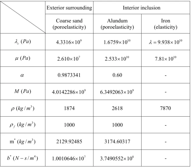
The material properties in the exterior and interior media are converted from Zimmerman and Stern (1993a) and Yew and Jogi (1978), respectively. The corresponding material constants are listed in Table I. Since we adopt a special type of the incident wave defined in Eq. (86), the series representation of the field associated with the indexes σmn is reduced merely to a single one ( , , ) (1,3,5)σ m n = . With the aid of Eqs. (53) and (55), we can get the simpler forms,
4 ( ) ( , ) ( ) 135 135,135 135 1 4 ( ) ( , ) ( ) 135 135,135 135 1 , ˆ . a i f c i f α α β β β α α β β β = = = = −
∑
∑
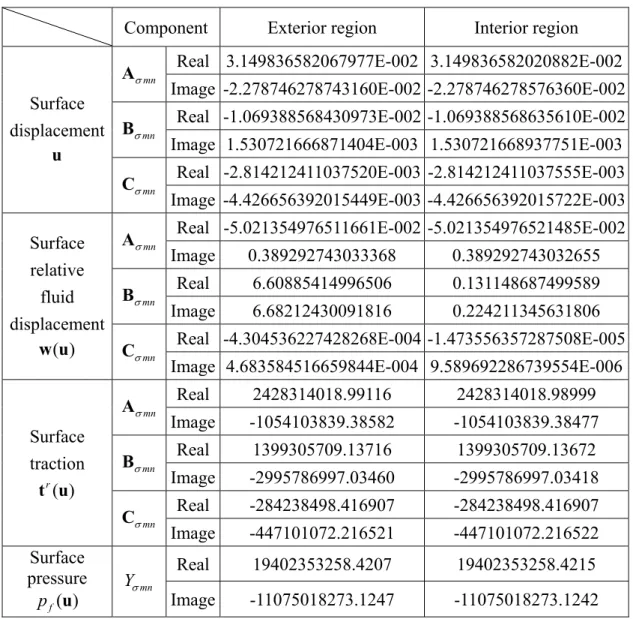
Q Q (87)frequency be ω =400 rad / secπ . Based on the series representations in Eqs. (45)-(46), we obtain the surface displacement, traction, and pore pressure fields in the exterior surrounding. By the same way, we use Eq. (47) to obtain those in the interior region. These results are represented through the composition of three mutually perpendicular vectors Aσmn, Bσmn, and Cσmn in Table II. For example: the exterior surface displacements can be written as follows,
-2 -2 -2 -3 -3 -3 ( , , ) (3.149836582067977 10 2.278746278743160 10 ) ( 1.069388568430973 10 1.530721666871404 10 ) +( 2.814212411037520 10 4.426656392015449 10 ) , mn mn mn a i i i σ σ σ θ φ + = × − × + − × + × − × − × u A B C (88)
and the exterior pressure as
( , , ) (19402353258.4207 11075018273.1247 )pf+ aθ φ = − i Yσmn. (89) The final value of the displacements at any point ( , , )aθ φ on the interface may be calculated by assigning the associated coordinates θ and φ to the vectors Aσmn,
mn
σ
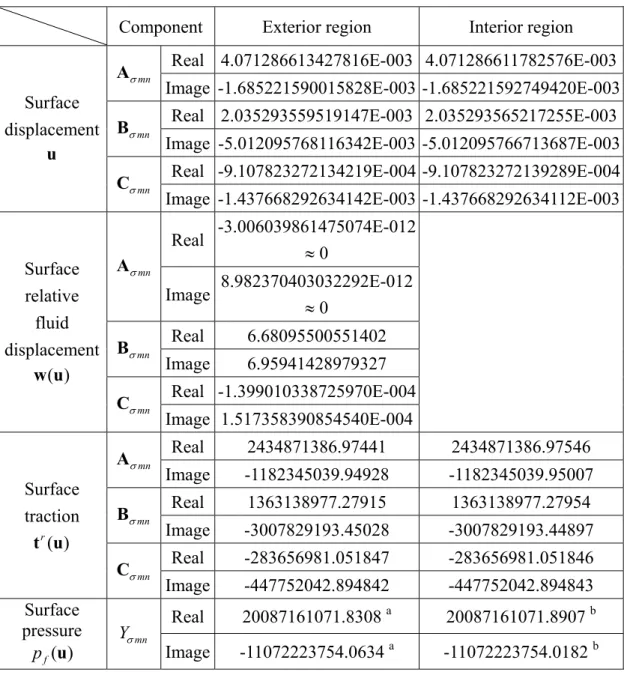
B , and Cσmn. On the other hand, we also tested the continuity condition at the interface for the elastic inclusion case subjected to the same incident wave. The material properties of this elastic inclusion are listed in Table I. The displacement and traction fields approaching from inside or outside are shown in Table III. Notice that the tangential relative fluid displacement and the pressure at the interface are not equal to zero. From Tables II and III, we can observe that the data for the displacements, tractions, and pressure at the interface indeed satisfy the conditions of the continuity with high accuracy.
B. A spherical inclusion subjected to a plane compressional wave
Stern (1993a) for the case of an elastic inclusion embedded within a poroelastic medium. In another case, we consider a poroelastic inclusion instead. The normal tractions at the interface and the displacements along the z-axis were calculated for both cases.
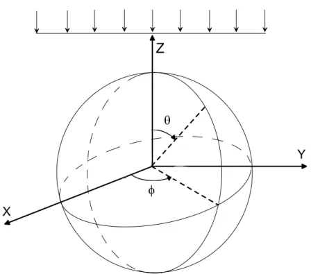
For an incident plane compressional wave impinging on the inclusion, the incident coefficients for the transition matrix can be obtained by Eq. (50). Let the incident wave be a fast dilatational plane wave with a wave number k and the p1 incident wave travel along the negative z-direction. Therefore, the incident wave with unit amplitude travels from top to bottom to the inclusion as shown in the Fig. 2. The potential of this plane wave can be represented as,
1( ) 0 1 1 . p ik z a i ϕ e ϕ μ − = (90)
With the series expansion, the exponential term can be expanded into the series of the spherical Bessel function and the Legendre polynomials (Ying and Truell, 1956) as
1 1 1 0 0 1 1 0 1 1 (2 1) ( ) (cos ) , p p p ik z ik a ik a i n n p n n e e e n i j k R P ϕ ϕ ϕ θ μ μ ∞ − − = = =
∑
+ (91)where (cos )Pn θ is the Legendre polynomials (i.e., m(cos ) n
P θ with m=0). At the same time, we set σ =1 (even) through comparing Eq. (91) with the spherical surface harmonics in Eq. (25). Thus the associated displacement fields are obtained from Eqs. (8) and (18),
1 1 1 (1) 0 0 1 0 0 1 ˆ ( ik zp ) ik ap p ik ap (2 1) . i n n n k e e e n i ϕ ϕ μ ∞ − − = = ∇ =
∑
+ u u (92)Substituting Eq. (92) into Eq. (50), we obtain the incident coefficients, 1 ( ) 0 (2 1) 1, 1, 1, 0 , and , 0, otherwise . p ik a n p mn e n i k m n N aσα ϕ μ α σ − ⎧ + = = = ∈ ⎪ = ⎨ ⎪⎩ (93)
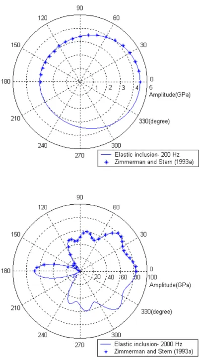
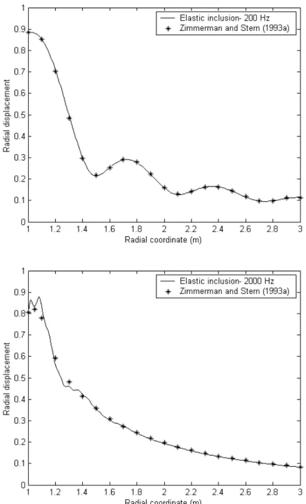
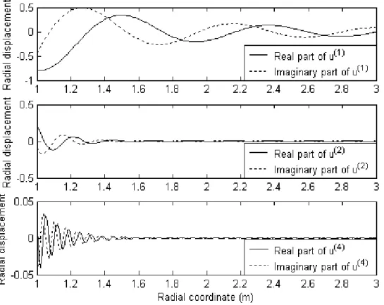
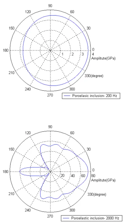
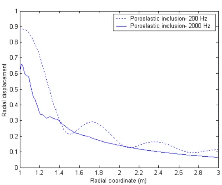
All results pertain to a spherical inclusion with a=1.0m. Figures 3 shows the surface normal tractions on the elastic inclusion at a low frequency 200Hz and at a high frequency 2000Hz, respectively. Figure 4 shows the amplitudes of the scattered wave along the z-axis at the two frequencies. The results obtained by Zimmerman and Stern (1993a) are also plotted by the symbol ‘*’ in Fig. 3 and 4. The differences are negligible except those in the region near the interface at 2000Hz. In fact, the amplitude obtained from Eq. (43) consists of four parts: u , (1) u , (2) u , and (3) u . (4) Under the incidence of the fast dilatational plane wave, the contribution of the mode conversion for the third part u is zero. The details of the second and fourth parts in (3) the region near the interface plotted in Fig. 5 show that the curves sway stronger and their phases change faster. As a result of the constructive and destructive phase interference, the curve for the radial amplitude in the region near the interface seems to be rough and irregular as shown in Fig. 4. Figure 6 presents the results for the surface normal tractions for the poroelastic inclusion at a low frequency 200Hz and at a high frequency 2000Hz. The patterns in this case are more obscure than those in elastic case. The results shown in Fig. 7 display the amplitudes of the radial displacements for the scattered waves along the z-axis at the two frequencies. The swaying region for the curve at 2000Hz is due to the interference which has been discussed in the elastic inclusion case.
V. CONCLUDING REMARKS
A solution based on the transition matrix for the scattered wave has several advantages especially for scatterers with an arbitrary shape because this approach can match the surface boundary conditions geometrically. However, to apply the transition matrix method, it is necessary to construct a set of complete and orthogonal basis
functions satisfying the three orthogonality conditions.
In this paper we adopt the approach introduced by Pao (1978) for elastic scattering problem to develop the transition matrix for the analysis of the scattering problem in poroelastic medium. A set of basis functions for a poroelastic medium are presented. The related orthogonality conditions are obtained by applying Betti’s third identity generalized for the poroelasticity and the transition matrix is derived accordingly. In order to show its validity and accuracy, this transition matrix is employed to analyze the wave scattered by an elastic spherical inclusion embedded in a poroelastic medium.
Although it appears that solving the scattering problem for a poroelastic inclusion is more complex than that for the elastic one. However, in our opinion, the analysis of the poroelastic inclusion problem by applying the transition matrix approach is actually easier than the elastic inclusion case because the conditions at the interface of the latter one are the degenerated case of the former one.
Some illustrative numerical results show that the regions near the interface present strong interferences which are caused by the coupling effect of the dilatational and rotational waves. This phenomenon can be explained by the reflection of the coupling waves. In addition, the amplitude of the radial displacement increases rapidly when the receiver approaches to the interface. The difference between the elastic and poroelastic inclusion shows that the amplitudes of normal traction for the elastic case are larger with more definite patterns.
ACKNOWLEDGEMENTS
The authors gratefully acknowledge the financial support granted by the National Science Council, R.O.C., (NSC-091-2211-E-002-080). The facility of calculation provided by National Taiwan University is also highly appreciated. We also thank the referees for their valuable criticisms and suggestions.
APPENDIX A: NORMALIZING TO THE DILATATIONAL WAVES
This appendix presents the normalizing procedure for the dilatational waves. The determinant of the coefficients from the characteristic equation in Eq. (10) is set to zero as 2 2 2 2 2 2 2 2 (2 ) 0 . c f f m k k M k k M M ρ μ λ ρ α ω ω ρ α ρ ω ω − + − = − − (A.1)
Equation (A.1) provides the characteristic values as
2 2 2 1 2 2 2 2 ( 4 ) 2 , ( 4 ) 2 . p p k B B AC A k B B AC A ω ω = − − = + − (A.2)
where A , B , and C are defined in Eq.(12). Substitution of Eq. (A.2) into (A.1) gives two corresponding characteristic vectors,
2 2 1 1 1 2 2 2 2 2 2 2 2 2 , 1 ( ) ( ) , 1 , 1 , 1 , [ ( 2 ) ] ( ) . T T p p m f T T p p c f k k M M k k M μ ρ ρ α ω ω μ ρ λ μ ρ α ω ω = − − − = − − + − (A.3)
In order to normalize Eq. (10), we rewrite the parameters μ1 and μ2 shown in the preceding equations in a common denominator form,
2 2 2 2 1 2 1 2 1 2 2 2 2 2 2 2 2 2 1 1 2 2 2 2 2 2 ( )( ) [( )( )] , [ ( 2 ) ]( ) [( )( )] , p p p p m f f f p p p p c f f f k k k k M M M M k k k k M M M μ ρ ρ α ρ α ρ α ω ω ω ω μ ρ λ μ ρ α ρ α ρ α ω ω ω ω = − − − − − = − − + − − − (A.4)
where Eq. (A.4) can be further simplified to the equations presented in Eq. (15). The normalized matrices corresponding to Eq. (10) are expressed as:
2 1 1 1 1 2 2 2 1 1 2 2 2 2 * 1 1 * 2 2 ( 2 ) 2 ( 2 ) , ( 2 ) ( 2 ) 2 1 ( 2 ) 1 ( 2 ) 0 1 1 0 c c c c T c c M M M M M M M M M M M M M M λ μ μ α μ λ μ μ α μ μ α μ λ μ μ α μ μ α μ λ μ α μ μ μ λ μ α μ λ μ μ α μ + + + + + + + = + + + + + + + + ⎡ + ⎤ ⎡ ⎤ ⎡ ⎤⎡ ⎤ ≡ ⎢ ⎥ ⎢ ⎥ ⎢ ⎥⎢ ⎥ ⎣ ⎦ ⎣ ⎦ ⎣ ⎦ ⎣ ⎦ ⎡ ⎤ ⎢ ⎥ ⎣ ⎦ (A.5) and * 1 1 * 2 2 2 1 1 1 1 2 2 2 1 1 2 2 2 2 1 1 0 1 1 0 2 . 2 T f f m m f m f f m f f m f m ρ ρ μ μ ρ ρ ρ μ μ ρ ρμ ρ μ ρ ρμ ρ μ μ ρ ρ μ ρμ ρ μ μ ρ ρ μ ρ ρ μ ρ μ ⎡ ⎤ ⎡ ⎤ ⎡ ⎤⎡ ⎤ ≡ ⎢ ⎥ ⎢ ⎥ ⎢ ⎥⎢ ⎥ ⎣ ⎦ ⎣ ⎦⎣ ⎦ ⎣ ⎦ ⎡ + + + + + ⎤ = ⎢ + + + + + ⎥ ⎢ ⎥ ⎣ ⎦ (A.6)
With the aid of the following equation,
2 2 2
4ac d− = −2b +2b b +4ac , (A.7) the symmetric off-diagonal elements of Eq. (A.5) vanish,
1 1 2 2
(λc+2 )μ μ α μ μ α+ M + M M+ μ =0 , (A.8) in which the analogous condition has not been presented in Kargl and Lim’s paper.
Through the aid of the equation as shown below, 2 4 2 4 ,
b + ac B= − AC (A.9)
the element (1,1) of Eq. (A.5) is given by
2 2 * 2 2 2 1 ( 2 ) [ 4 ][ ( 2 ) p ] , c c k A B AC c λ μ ρ λ μ ω + = − − − + (A.10)
and the element (2,2) of Eq. (A.5) is given by
2 1 * 2 2 2 1 4 ( p ) . m k M A B AC M a ρ ω = − − (A.11)
Based on the definitions of Eqs.(12) and (14), we have the diagonal elements of Eq. (A.6), 2 2 1 2 * 2 2 2 4 [ ( 2 ) 2] , p p c k k A B AC c ρ ρ λ μ ω ω = − − − + (A.12)
2 2 2 1 * 2 2 2 4 ( 2) , p p m m k k A B AC M a ρ ρ ω ω = − − (A.13)
and show that the symmetric off-diagonal elements of Eq. (A.6) are zero. Furthermore, we also use some algebraic techniques to obtain the following identities among the factors: μ1, μ2, and μ3. 1 1 2 2 1 3 1 2 2 2 2 3 2 2 ) ( ( ) ( 1) 0 , 2 ( ) ( ) 0 . c s p c s p M k k M M k k M μ λ μ α μμ μ αμ λ μ μ α μ μ α μ + + − + + = + + − + + = (A.14)
These results will be useful in the evaluation of Eq. (B.17) and the analogous conditions have not been presented in Kargl and Lin’s paper.