A Simple Multiloop Tuning Method for PID Controllers with No Proportional Kick

(1)

Industrial & Engineering Chemistry Research is published by the American Chemical Society. 1155 Sixteenth Street N.W., Washington, DC 20036

Article

A Simple Multiloop Tuning Method for

PID Controllers with No Proportional Kick

I-Lung ChienHsiao-Ping Huang, and Jen-Chien Yang

Ind. Eng. Chem. Res., 1999, 38 (4), 1456-1468 • DOI: 10.1021/ie980595v

Downloaded from http://pubs.acs.org on November 18, 2008

A Simple Multiloop Tuning Method for PID Controllers with No

Proportional Kick

I-Lung Chien*

Department of Chemical Engineering, National Taiwan University of Science and Technology, Taipei, Taiwan 106, Republic of China

Hsiao-Ping Huang and Jen-Chien Yang

Department of Chemical Engineering, National Taiwan University, Taipei, Taiwan 106, Republic of China

A simple tuning method for multiloop PID controllers will be presented in this article. The method is suited for PID algorithms with no proportional and derivative kick. This tuning method is derived from a controller synthesis method with a control performance specification of 5% overshoot on servo response. Depending on the interaction natures of the multiloop systems, tuning based on the diagonal elements of the model or further detuning may be necessary. For

systems with a relative gain array [RGA(λii)] < 1, a detuning factor based on this information

is proposed. The information needed for controller tuning purposes is the dynamic model parameters of the diagonal elements and the process gain information of the off-diagonal elements. The tuning method procedure is very simple and straightforward, utilizing only nth identification tests with n as the number of the interacting control loops. The tuning method can easily be applied to various industrial situations with almost no need for a priori process knowledge.

1. Introduction

Although many advanced control concepts have been introduced within the last 20 years, the vast majority of the controllers in industry are still of the PID type. For this reason, the proper tuning of the PID controllers so that they can perform to their expectation is an important factor for successful plant operation. There are many controller tuning methods proposed in the literature, but most of them only consider simpler SISO (single-input, single-output) systems. When loop inter-actions exist among the control loops, the otherwise acceptable control performance of SISO environments may quite often deteriorate to even unstable situations. That is why, for multivariable systems, the tuning of a multiloop PID controller has to bring loop interactions into consideration. A common way to handle this problem is to introduce a detuning factor to the SISO tuning constants to stabilize the multivariable closed-loop system. If the process model of the multivariable system is available, a systematic procedure to find this detuning factor is suggested in the literature for

mul-tiloop PI tuning by Luyben.1 _{Friman and Waller}2

suggested the use of autotuning by a relay feedback method to establish a multivariable process model and the use of a trial-and-error procedure to determine the

detuning factor. Shen and Yu3_{utilized sequential relay}

feedback identification to obtain the frequency response information of a multivariable system and to use de-tuned Ziegler-Nichols tuning rules to handle the loop

interactions. Loh et al.4_{used a sequential identification}

method similar to that of Shen and Yu3 _{but proposed}

the use of a modified PID algorithm with an additional

β parameter to decrease the interactions among control

loops. Palmor et al.5_{and Halevi et al.}6_{proposed not to}

use a sequential relay identification method but instead used simultaneous relays on all of the control loops during the identification stage. They obtained the desired critical point information from their experiment after several iterations and then used regular or modi-fied Ziegler-Nichols tuning rules for control.

All of the tuning methods mentioned above had to obtain the process model or the frequency response information in “several rather long” experiments. In this paper, an alternative, very simple multiloop PID Tuning method is proposed. The method is suited for a PID algorithm with no proportional and derivative “kicks”. This tuning method is derived from a controller syn-thesis method with a control performance specification of 5% overshoot of the servo response. Depending on the interaction natures of the multiloop systems, controller tuning based on the diagonal elements of the model or further detuning may be necessary. For systems with

a relative gain array [RGA(λii)] < 1, a detuning factor

based on this information is proposed. The information needed for controller tuning purposes includes the dynamic model parameters of the diagonal elements and the process gain information of the off-diagonal ele-ments. The tuning method procedure is very simple and straightforward, utilizing only nth identification tests with n as the number of the interacting control loops. The tuning method can easily be applied to various industrial situations with almost no need for a priori process knowledge.

Various distillation dual-point control examples with

RGA(λii) > 1 and two other examples, including an

industrial reactor control example with RGA(λii) < 1 and

one 3 × 3 example, will be used to demonstrate the

superior performance of this tuning method. Both set-point and load disturbance response will be examined. * To whom all correspondence should be addressed. Phone:

+886-2-2737-6652. Fax: +886-2-2737-6644. E-mail: Chien@ ch.ntust.edu.tw.

(3)

2. The Tuning Method

In a standard PID controller, because the proportional mode is acting on the error signal, there will be a large kick of the controller output during setpoint changes. If the multiloop control system has large interactions among the loops, the large controller action on one loop will be a large load disturbance to the other loops. To reject this large load disturbance, the corrective action by the controllers in other loops will also be large, causing disturbance back to the loop with setpoint changes. The disturbance effect will go back and forth among the control loops, causing control problems.

For this reason, an obvious solution is to not let the control action have the kick at the time of the setpoint changes. This calls for a PID form with no proportional kick, which simply means having the proportional mode acting on the negative sign of the controlled variable alone. The Laplace transform representation of this control is

In the PID form above, it is customary to have the derivative mode also acting on the negative sign of the controlled variable to prevent a derivative kick. Also note that this PID form can be found in almost every industrial distributed control systems, thus no special control implementation is needed.

This PID form in eq 1, on one hand, will not have an initial proportional kick, but on the other hand, the closed-loop servo response will be sluggish if the same PID tuning constants derived from a standard PID form is used. For this reason, the PID tuning rules need to be modified for this particular PID form. We will use controller synthesis method to derive the PID controller tuning parameters. In the following, the derivation of the tuning rules will be divided into two parts by obtaining PI tuning rules and PID tuning rules. For controlled variables with noisy signals, PI tuning rules with no derivative action can be selected.

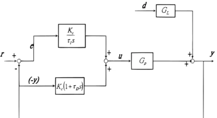
2.1. PI Tuning Rules. We will start our discussions by considering a single-loop control system. For a closed-loop system with a PID controller with no proportional kick (see Figure 1), the relationship between the con-trolled variable (y) and the setpoint (r) is as follows (dropping the Laplace transform variable s for simplicity reason):

Gpis the model of the process for controller tuning

purposes. We will classify the processes into two cat-egories.

2.1.1. Time Constant Dominant Processes. Most of the difficult control loops in the chemical industry are of this type with the dominant time constant of the system greater than 5 times the process deadtime. If this holds, the proper process model for controller tuning purposes will have the following integrating plus dead-time form:

where R is the slope of the initial unit step response of the controlled variable and L is the process apparent deadtime. If a first-order plus deadtime model is

ob-tained from some model identification steps with Kpas

the process gain,τ as the process time constant, and L

as the process deadtime, for (L/τ) < 0.2, the

approxima-tion of calculating R to be equal to (Kp/τ) will be used.

In order to derive PI tuning parameters, the deadtime term in eq 3 needs to be approximated using a first-order Taylor series, thus

Substituting eq 4 into eq 2 and simplifying, we obtain

The closed-loop servo response is a second-order re-sponse. Let’s assume our desired closed-loop servo response to be an underdamped system with a damping

coefficient (ζ) of 0.707. This corresponds to a closed-loop

system with about 5% overshoot. The desired closed-loop servo response is

where τcl is a user-specified closed-loop effective time

constant. Equating eqs 5 and 6, we can obtain the PI tuning rules as

2.1.2. Deadtime Important Processes. For

pro-cesses with a deadtime greater than1_/

5 of the process

time constant, it is better for controller tuning purpose to model the processes as a first-order plus deadtime model. With the same Taylor approximation, the process model becomes

Substituting eq 9 into eq 2 and simplifying, we obtain

Figure 1. Block diagram of PID control loop with no proportional

kick.

u(s) ) Kc{-y(s) + (1/τis)E(s) +τds[-y(s)]} (1)

s + 1 (10)

(4)

Again, it is a second-order response. With the same desired closed-loop servo response as previously eq 6, we can obtain the PI tuning rules as

Normally, we would specifyτcl to be smaller than the

open-loop time constant,τ; thus, the negative terms in

eqs 11 and 12 will not create any problems in changing

the signs of Kcandτi.

2.2. PID Tuning Rules. The derivation of the PID tuning parameters is similar to the above PI derivation except that the deadtime approximation is a little more accurate because of the use of the first-order Pade´ approximation. In this case, then, the apparent dead-time terms in integrating plus deaddead-time or first-order plus deadtime models can be approximated to be

We will use the same classification of the process model and the same closed-loop specification as in the above PI tuning rule derivation. The resulting PID tuning rules with detail derivation can be found in the Ap-pendix.

3. Multiloop Considerations

In the above sections, we have developed the PI/PID tuning rules on the basis of a controller synthesis method. We have also assumed that by using PI/PID form with no proportional kick the interactions among the control loops will be considerably reduced. For a

multiloop situation, the relationship between yiand ui

is not simply the diagonal element of the process model

matrix. Let’s take a 2 × 2 system as an illustrating

example. For a 2 × 2 closed-loop control system, the

process transfer function between y1and u1while loop

2 is on manual is

On the other hand, the relationship between y1and u1

while loop 2 is on automatic mode is (cf., Shen and Yu3₎

whereκ is the Rijnsdorp interaction measure7 _{and h}

2

is the complementary sensitivity function for loop 2. The

κ and h2are defined as

and

The above relationship in eq 15 holds also for PID controller with the form of no proportional kick.

Assuming that the controller tuning parameters are chosen so that the complementary sensitivity function

(h2) is a stable system with unity gain, then by

calculat-ing the high- and low-frequency asymptotes of eq 15 we can have some idea of how the loop interactions affect the open-loop transfer function. For individual process transfer function to be assumed as a first-order plus deadtime model, at high frequency, this model is ap-proaching integrating plus deadtime form as in eq 3 and at low frequency this model is approaching a pure gain model. The following results are obtained:

because for controller design or tuning purposes, the process open-loop initial response (or high-frequency) behavior is the most important (as pointed by others;

see: Skogestad and Moraris,8,9_{Chien and Fruehauf,}10

and Chien and Ogunnaike11_{). In addition, from}

fre-quency asymptote analysis, the initial response of a particular control loop with the other loop in manual or automatic is known to be very similar in nature (from eqs 14 and 18). For these reasons, multiloop controller tuning based on the process model parameters in the main loop should provide satisfactory closed-loop re-sults.

For systems with RGA(λii) < 1, special consideration

should be taken to avoid having overly aggressive controller action. From eq 19, the process transfer function is adjusted by multiplying a factor with values

greater than one [reciprocal of RGA(λii)] at low

frequen-cies. Using the tuning rules based on the open-loop

transfer function, Gii, will be too aggressive at

low-frequency ranges. To obtain PID controller tuning parameters which will not be too aggressive in all frequency ranges, a reasonable choice is to introduce an

extra detuning factor with the value of RGA(λii) to

detune Kc as well as τi, and τd parameters in the

following matter:

From the definition of RGA(λii), we can also see that

further detuning is necessary for systems with RGA-(λii) < 1. The RGA(λii) is defined as12

Thus, if RGA(λii) < 1, this means that the effective

process gain of the main loop will be increased if the other loops are closed. Therefore, any controller tuning methods only based on the information of model pa-rameters in the main loop will be too aggressive. This calls for an extra detuning factor. The value of the detuning factor should be related to the closeness of the

) G11 RGA(λii) (19)

Kc) (Kc)based on main loopRGA(λii) (20)

τi)

(τi)based on main loop

RGA(λii)

(21)

τd) (τd)based on main loopRGA(λii) (22)

λii)

(

∂yi

∂ui

)

other loops opened

/

(

∂yi

∂ui

)

other loops closed

(5)

open-loop process gain to the process gain when the other loops are closed. For this reason, the detuning rules in eqs 20-22 are justified.

The choosing of the user-specified closed-loop effective

time constant, τcl, is a matter of trading off between

control loop performance and robustness. Ifτclis chosen

to be smaller, then the controller performance is faster, but the control action is more vigorous, and the model

mismatch tolerance is worse. On the other hand, ifτcl

is chosen to be larger, the controller performance is more sluggish, but the control action will be smoother, and the model mismatch tolerance is better. With many multiloop system simulations, the following selection of

τclin Figure 2 was determined empirically, which gave

satisfactory closed-loop response under both nominal and reasonable model mismatch conditions.

The reason for choosingτclto be smaller for first-order

plus deadtime model when L/τ > 0.5 is because for

dead-time dominant processes with large L values selecting

τcl) nL with n as number of interacting control loops

will give overly sluggish closed-loop responses. For L/τ

> 1.0, a PID controller will be sluggish anyhow. In this circumstance, a deadtime compensation scheme such as the Smith predictor will be more beneficial.

The resulting PI tuning rules for a 2× 2 system can

be found in Table 1. From the process model information obtained from model identification steps, the PI tuning

parameters can easily be calculated. For a 3× 3 or 4 ×

4 system, the PI tuning parameters can be calculated

in a manner similar to that of Table 1 by selectingτcl

as in Figure 2 and using eqs 7, 8, 11, and 12 to calculate

Kcandτi. Similarly, the PID tuning parameters for a 2

× 2 system can easily be calculated with the selection

ofτclas in Figure 2. The results can be seen in Table 2

once the model parameters are known. For a 3× 3 or 4

× 4 system, the PID tuning parameters can be calcu-lated in a similar matter.

In calculating the controller tuning parameters, any suitable model identification schemes such as the

biased-relay method proposed by Huang et al.13_{can be}

used to obtain the necessary information by just using

nth relay feedback test with n as the number of the

interacting control loops. For systems with RGA(λii) >

1, the PI/PID tuning rules can directly be calculated by

using the model parameters (R, L, Kp, andτ) in the main

loops. As for systems with RGA(λii) < 1, additional

information of the process gains in the off-diagonal elements are also needed. The biased-relay method

proposed by Huang et al.13 _{is suitable for calculating}

the process gains because these values can be obtained

by calculating the ratio of two integrals in yi(t) and uj

-(t) for each cycle of the test result and then taking the average of several cycles.

Table 1. PI Tuning Rules for PID Controller with No Proportional Kick (2_{× 2 system)}a

(L/τ) < 0.2 0.2 < (L/τ) < 0.5 (L/τ) > 0.5 Kc 1/2.045RL 1 K_p (1.414m + 1) - m2(L/τ) (m2+ 1.414m + 1)(L/τ) 1 K_p 2.414 - (L/τ) 3.414(L/τ) τi 3.828L τ (1.414m + 1)(L/τ) - m2(L/τ)2 1 + (L/τ) τ 2.414(L/τ) - (L/τ)2 1 + (L/τ)

a_{For the cases when 0.2 < (L/}_{τ) < 0.5, m ) 2 - [(L/τ) - 0.2]/0.3 is used.}

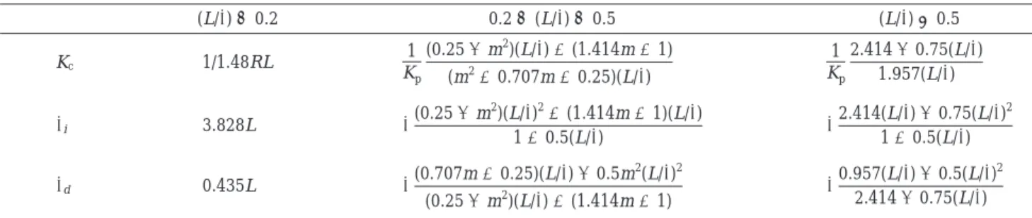
Table 2. PID Tuning Rules for PID Controller with No Proportional Kick (2× 2 system)a

(L/τ) < 0.2 0.2 < (L/τ) < 0.5 (L/τ) > 0.5 Kc 1/1.48RL 1 K_p (0.25 - m2)(L/τ) + (1.414m + 1) (m2+ 0.707m + 0.25)(L/τ) 1 K_p 2.414 - 0.75(L/τ) 1.957(L/τ) τi 3.828L τ (0.25 - m2)(L/τ)2_{+ (1.414m + 1)(L/τ)} 1 + 0.5(L/τ) τ 2.414(L/τ) - 0.75(L/τ)2 1 + 0.5(L/τ) τd 0.435L τ (0.707m + 0.25)(L/τ) - 0.5m2(L/τ)2 (0.25 - m2)(L/τ) + (1.414m + 1) τ 0.957(L/τ) - 0.5(L/τ)2 2.414 - 0.75(L/τ)

a_{For the cases when 0.2 < (L/}_{τ) < 0.5, m ) 2 - [L/τ - 0.2]/0.3 is used.}

(6)

The overall tuning procedure is summarized in the following:

1. With all loops in manual mode, one can apply identification tests on loop 1 and collect dynamic data

on u1versus y1and u1versus yi,i*1.

2. By using any suitable identification method, one can obtain first-order plus deadtime model parameters

for G11and process gain information, Kpi1, i*1.

3. Similar test apply to other loops and give first-order plus deadtime model parameters for all of the diagonal elements in the process model matrix and gain informa-tion for all of the off-diagonal elements.

4. If RGA(λii) > 1, only model parameters in Giiwill

be used in the tuning rules.

5. With RGA(λii) > 1, one can calculate L/τ for each

loop. For the cases with (L/τ) < 0.2, R () Kp/τ) can be

calculated in each loop. For each L/τ range, PI/PID

tuning parameters can be calculated from appropriate columns in the tables mentioned in this section.

6. If RGA(λii) < 1, a detuning factor equal to

RGA(λii) can be calculated from the model

param-eters.

7. With RGA(λii) < 1, the controller tuning parameters

can be further detuned via eqs 20-22.

(7)

8. With the tuning parameters calculated, a PI/PID controller can be implemented with no proportional and derivative kick in your plant.

This proposed tuning method is suitable for all normal multiloop control applications. For the situation when

a multiloop control system has RGA(λii) < 0, the

recommendation is to switch the pairings so that

RGA-(λii) will become greater than 0. From the definition of

RGA in eq 23, the sign of the controller action will be reversed when the other loops are in automatic or in

manual in the situation when RGA(λii) < 0. This means

that even if the multiloop control system is tuned properly to be stable in the automatic mode, any failure in the loops in the system which causes the loops to enter a manual mode will destabilize the overall control system. The control integrity is unacceptable for a RGA-(λii) < 0 system.

4. Simulation Results

Many 2× 2 systems and several 3 × 3 systems have

been used to test the closed-loop performance of the proposed tuning method above. All give very satisfactory responses. In the following, we will present the results

on a simulated column control system with RGA(λii) >

1 and one reactor control example with RGA(λii) < 1 as

well as a 3× 3 example.

Example 1. Wood and Berry Column.14_The

trans-fer function model shown below is a pilot-scale distil-lation column model separating a mixture of methanol and water. This model has been discussed in a number

of other 2× 2 loop tuning studies, including those by

Luyben,1_{Loh et al.,}4_{Shen and Yu,}3_{and Palmor et al.}5

Wood and Berry14 _{reported the following empirical}

transfer function model:

The first step of the controller tuning procedure is to do two bias-relay feedback tests on loops 1 and 2. From the model identification results and from the fact that

this system has the characteristics of RGA(λii) > 1, no

detuning is necessary. The PI or PID tuning parameters can be calculated from Tables 1 or 2 respectively. The closed-loop setpoint and load responses using this proposed tuning method will be compared to the tuning

methods by Luyben,1_{Shen and Yu,}3_{Palmor et al.,}5_and

Loh et al.4_{The PI tuning parameters used in the above}

tuning methods are tabulated in Table 3.

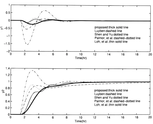
The closed-loop response for a setpoint change in y1

is shown in Figure 3a with the manipulated variable changes in Figure 3b. It is clearly shown in these two figures that controller tunings using PI controllers with no proportional kick (our proposed method and the one

by Loh et al.4_{) provide better closed-loop performance}

than the ones using standard PI controllers (Luyben,1

Shen and Yu,3 _{and Palmor et al.}5_{). Although the}

performance of Loh et al.4_{is satisfactory, the y}

2response

is more sluggish. In addition, the method of Loh et al. uses the more time-consuming “sequential” identifica-tion procedure for obtaining its tuning constants. The

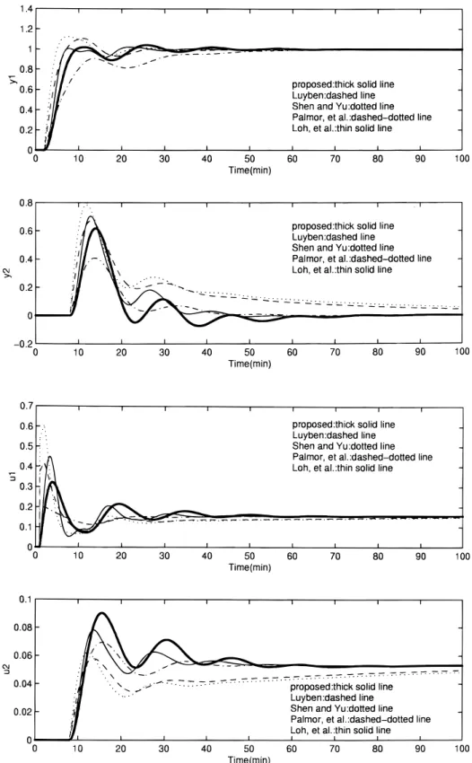
Figure 4. Closed-loop response for example 1 with y2setpoint change.

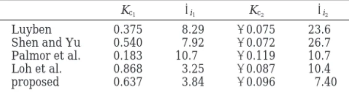
Table 3. PI Tuning Parameters for Wood and Berry Column Kc1 τi1 Kc2 τi2 Luyben 0.375 8.29 -0.075 23.6 Shen and Yu 0.540 7.92 -0.072 26.7 Palmor et al. 0.183 10.7 -0.119 10.7 Loh et al. 0.868 3.25 -0.087 10.4 proposed 0.637 3.84 -0.096 7.40

[

y1(s) y2(s)

]

)

[

12.8e-s 16.7s + 1 -18.9e-3s 21.0s + 1 6.6e-7s 10.9s + 1 -19.4e-3s 14.4s + 1

]

[

u1(s) u2(s)

]

+

[

3.8e-8.1s 14.9s + 1 4.9e-3.4s 13.2s + 1

]

[d(s)] (24)

(8)

manipulated variables of our proposed method are quite smooth, which is favorable in industrial applications.

Closed-loop responses for changes in setpoint of y2and

the load response with the disturbance, d, from 0 to 1 at t ) 1 can be found in Figures 4 and 5, respectively. Again, our proposed method reaches the setpoint the fastest in these two changes and is superior in com-parison to other tuning methods.

The comparison of the controller robustness property can be carried out by assuming the plant with an input

uncertainty∆ to describe modeling errors. The

closed-loop system is stable if and only if (cf., Morari and

Zafiriou15₎

whereσj(‚) is the maximum singular value of (‚) and H

is the complementary sensitivity function of the entire

closed-loop system. By plottingσj[H(iω)] versus ω for the

Figure 5. Closed-loop response for example 1 with load change.

Figure 6. Plot ofσj[H(iω)] vs ω for example 1.

σj[H(iω)] < 1

(9)

five tuning rules listed in Table 3, we can compare the robust stability of these five tuning rules. The tuning

method will be more robust if the value ofσj[H(iω)] is

smaller in all frequency ranges.

Figure 6 is a plot ofσj[H(iω)] versus ω for this system.

From this figure, we see that the proposed tuning

method is more robust than the method by Loh et al.4

for most frequencies but is less robust than the other three tuning methods for high frequencies. Even though

the robust stability property of the methods by Luyben,1

Shen and Yu,3 _{and Palmor et al.}5 _{are favorable, the}

nominal performances of these three tuning methods are considerably more sluggish, as shown in above Figures 3-5.

One of the criticisms of using σj[H(iω)] in robust

stability analysis is that the stability criterion may be too conservative. As an independent check, closed-loop results using the tuning constants as in Table 3 but with process parameters mismatch of +30% in diagonal gains and deadtime elements are simulated. Figure 7 shows

Figure 7. Model mismatch run for example 1 with y1setpoint change.

(10)

the setpoint change in y1under model mismatch

condi-tion. The proposed method still provides excellent closed-loop performance with this severe model

mis-match condition. The methods of Luyben,1 _{Shen and}

Yu,3 _{and Palmor et al.}5 _{are still stable because their}

controller actions are too sluggish during nominal

condition. The method by Loh et al.,4 _{although the}

nominal response is satisfactory, is much too oscillatory under this model mismatch condition. Considering the

trade-off between loop performance and robustness, the proposed tuning method is the most favorable.

In order to further improve the closed-loop response, a controller with an additional derivative mode can be considered if the process variable measurements are not very noisy. The PID tuning parameters for this column

can be calculated from Table 2 to be Kc1) 0.881, τi1)

3.84,τd1) 0.436, Kc2) -0.136, τi2) 8.24, and τd2) 1.23.

The closed-loop response of the PID controller with no

Figure 9. Closed-loop response for example 2 with y1setpoint change.

(11)

proportional kick using the proposed tuning method is comparing to the response of a PI controller in Figure

8 for a setpoint change in y1. The closed-loop

perfor-mance of PID controller is further improved.

Example 2. A Reactor Control Problem. The second example is an industrial-scale polymerization reactor control problem. In order to improve the product quality consistency, a control improvement project is initiated for which the first phase of the project is to do automatic reactor condition control. The manipulated variables of this control tier are the setpoints of various reactor feed flow control loops. The control hierarchy proposed is similar to Figure 30.25 in Ogunnaike and

Ray.16 _{The future higher tier product quality control}

loops will be setting the setpoints of the reactor condi-tion control loops.

For proprietary reasons, we will not describe in detail this reactor control system. The process model for the reactor condition control loops is obtained from model identification to be

The time scales are in hours, so the process dynamic response is quite slow. The two controlled variables are two measurements representing the reactor condition, and the two manipulated variables are the setpoints of two reactor feed flow loops with load disturbance as the purge flow of the reactor.

Notice that in this case the interactions is such that

RGA(λii) < 1 thus further detuning is necessary. When

the tuning procedure in the above section is followed, the detuning factor for this system is 0.709. The resulting PI tuning parameters together with the tuning parameters calculated using other tuning methods are tabulated in Table 4.

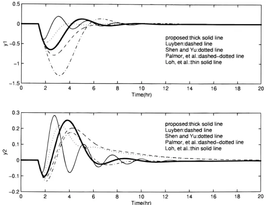
Figures 9-11 show the closed-loop responses for this

system under setpoint change of y1, setpoint change of

y2, and load disturbance changes, respectively. Again,

the proposed method provides satisfactory closed-loop performance with the minimum identification tests needed.

Various other 2× 2 systems have been used to test

the adequacy of this proposed method. They are

For RGA(λii) > 1 systems, TS, VL, and WW models

in Luyben,1_{and a column model in Taiwo.}17

For RGA(λii) < 1 systems, a process model in

Nied-erlinski18_{with higher order process model.}

Our proposed tuning method performs all quite satisfactory.

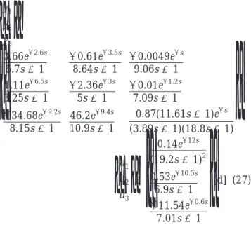
Example 3. A 3 × 3 System. A 3 × 3 example

originated in Ogunnaike and Ray19_{and later studied}

by Luyben1_{and Halevi et al.}6_{will be used here to test}

[

y1(s) y2(s)

]

)

[

22.89e-0.2s 4.572s + 1 -11.64e-0.4s 1.807s + 1 4.689e-0.2s 2.174s + 1 5.80e-0.4s 1.801s + 1

]

[

u1(s) u2(s)

]

+

[

-4.243e-0.4s 3.445s + 1 -0.601e-0.4s 1.982s + 1

]

[d(s)] (26)

Table 4. PI Tuning Parameters for Reactor Control Problem Kc1 τi1 Kc2 τi2 Luyben 0.210 2.26 0.175 4.25 Shen and Yu 0.459 1.50 0.183 4.45 Palmor et al. 0.0978 1.60 0.375 1.60 Loh et al. 0.620 0.60 0.247 1.78 proposed 0.263 1.42 0.163 1.77

Table 5. PI Tuning Parameters for ex 3

Kc1 τi1 Kc2 τi2 Kc3 τi3

Luyben 1.51 16.4 -0.295 18.0 2.63 6.61 Shen and Yu 2.55 16.5 -0.235 26.1 3.39 7.39 Halevi et al. 1.25 10.5 -0.339 10.5 0.923 10.5 proposed 1.08 4.25 -0.233 3.32 2.78 5.24

(12)

the performance of the proposed method for systems with control loops greater than two. The process model is

This 3× 3 system has RGA(λii) elements all greater

than one; thus, no further detuning is necessary. By

application of the bias-relay tests to obtain the model parameters of the three diagonal elements of the process, the PI tuning parameters can be calculated using the procedure outlined in Section 3. The resulting PI tuning parameters together with the tuning param-eters reported in the literatures for other tuning meth-ods are tabulated in Table 5.

Figure 12 illustrates the closed-loop response for this system under load disturbance. The closed-loop perfor-mance of the proposed method is excellent. Similar good performance can be found for setpoint changes in all three controlled variables.

5. Conclusions

In this paper, a very simple PID tuning method is proposed for multiloop control systems. The tuning method is based on the PID controller implementation with the form of no proportional kick. With this con-troller form, the interactions between the control loop can be minimized, and the desired closed-loop perfor-mance can still be specified by controller synthesis method. Depending on the interaction natures of the multiloop systems, controller tuning based on the diagonal elements of the model or further detuning may

[d] (27)

(13)

factor based on the value of RGA(λii) is proposed. One

of the biggest advantage of the proposed tuning method is that because the tuning method only requires dy-namic model parameters of the diagonal elements and the process gain information of the off-diagonal elements only nth identification tests (with n as the number of the interacting control loops) are needed to determined the PID tuning parameters as opposed to other tuning methods which require more iterative tests. Because less interference of process operation is always prefer-able for industrial situations, this tuning method has the potential to be widely applicable in industry. Many simulation tests have confirmed the performance of this proposed tuning method. Its closed-loop servo and load responses are all very satisfactory.

Acknowledgment

This work is supported by National Science Council of the Republic of China under Grant NSC 87-2214-E-011-025.

Appendix: Derivation of PID Tuning Rules The closed-loop transfer function between controlled variable (y) and setpoint (r) is

For time constant dominant processes, the process

model, Gp, can be approximated using Pade´

approxima-tion as

Substituting eq A.2 into A.1 and simplifying, we get

Let us assume our desired closed-loop servo response to be a underdamped system with damping coefficient of 0.707. This corresponds to a closed-loop system with about 5% overshoot. The desired closed-loop servo response is

whereτclis an user-specified closed-loop effective time

constant. Equating eqs A.3 and A.4 and doing some algebraic manipulation, we can solve for the PID tuning parameters as

For processes with deadtime greater than 1_/

5 of the

process time constant, it is better for controller tuning purposes to model the processes as a first-order-plus deadtime model. With the same Pade´ approximation as

Substituting eq A.8 into A.1 and simplifying, we obtain

Again, equating eqs A.9 and A.4 and doing some algebraic manipulation, we can solve for the PID tuning parameters as

By selectingτcl as in Figure 2, the negative terms in

eqs A.10-A.12 will not cause any problem in changing

the signs of the PID tuning parameters. With the τcl

selection as in Figure 2, combining with eqs A.5-A.7 and A.10-A.12, the final PID tuning rules in Table 2 can be obtained.

Literature Cited

(1) Luyben, W. L. Simple Method for Tuning SISO Controllers in Multivariable Systems. Ind. Eng. Chem. Res. 1986, 25, 654.

(2) Friman, M.; Waller, K. V. Autotuning of Multiloop Control Systems. Ind. Eng. Chem. Res. 1994, 33, 1708.

(3) Shen, S.-H.; Yu, C.-C. Use of Relay-Feedback Test for Automatic Tuning of Multivariable Systems. AIChE J. 1994, 40, 627.

(4) Loh, A. P.; Hang, C. C.; Quek, C. K.; Vasnani, V. U. Autotuning of Multiloop Proportional-Integral Controllers Using Relay Feedback. Ind. Eng. Chem. Res. 1993, 32, 1102.

(5) Palmor, Z. J.; Halevi, Y.; Krasney, N. Automatic Tuning of Decentralized PID Controllers for TITO Processes. Automatica

1995, 31 (7), 1001.

(6) Halevi, Y.; Palmor, Z. J.; Efrati, T. Automatic Tuning of Decentralized PID Controllers for MIMO Processes. J. Proc. Cont.

1997, 7 (2), 119.

(7) Rijnsdorp, J. E. Interaction in Two-Variable Control Sys-tems for Distillation. Automatica 1965, 1, 15.

(8) Skogestad, S.; Morari, M. LV-Control of a High-Purity Distillation Column. Chem. Eng. Sci. 1988, 43, 33.

(9) Skogestad, S.; Morari, M. Understanding the Dynamic Behavior of Distillation Columns. Ind. Eng. Chem. Res. 1988, 27, 1848.

(10) Chien, I-L.; Fruehauf, P. S. Consider IMC Tuning to Improve Controller Performance. Chem. Eng. Prog. 1990, 86 (October), 33.

(11) Chien, I-L.; Ogunnaike, B. A. Modeling and Control of a Temperature-Based High-Purity Distillation Column. Chem. Eng.

Commun. 1997, 158, 71.

(12) Bristol, E. On a New Measure of Interaction for Multi-variable Process Control. IEEE Trans. Autom. Control 1966, AC-11, 133.

(13) Huang, H.-P.; Wang, G.-B.; Lee, M.-W.; Chien, I-L. Iden-tification of Transfer Function Models from the Relay Feedback Test. Chem. Eng. Commun. 1998, submitted.

(14) Wood, R. K.; Berry, M. W. Terminal Composition Control of Binary Distillation Columns. Chem. Eng. Sci. 1973, 28, 1707.

(15) Morari, M.; Zafiriou, E. Robust Process Control; Prentice-Hall: Englewood Cliffs, New Jersey, 1989.

(16) Ogunnaike, B. A.; Ray, W. H. Process Dynamics, Modeling,

and Control; Oxford University Press: New York, 1994.

(17) Taiwo, O. Application of the Method of Inequalities to the Multivariable Control of Binary Distillation Columns. Chem. Eng.

Sci. 1980, 35, 847.

(18) Niederlinski, A. A Heuristic Approach to the Design of Linear Multivariable Interacting Control Systems. Automatica

1971, 7, 691.

(19) Ogunnaike, B. A.; Ray, W. H. Multivariable Controller Design for Linear Systems Having Multiple Time Delays. AIChE

J. 1979, 25, 1043.

Received for review September 21, 1998 Revised manuscript received January 11, 1999 Accepted January 12, 1999 IE980595V