An Effective Tuning Method for Cysteine State Classification
Wei-Chun Chung, Chang-Biau Yang* and Chiou-Yi Hor
Department of Computer Science and EngineeringNational Sun Yat-sen University, Kaohsiung, Taiwan *Corresponding author: cbyang@cse.nsysu.edu.tw
Abstract—For solving the problem of cysteine state classification, we propose a 2-stage prediction method. In the first stage, we invoke the SVM to get the initial prediction. The features involved in SVM classification include the local profile PSSM, order of cysteines with the normalized protein length, physiochemical properties and structure probabilities. Then, in the second stage, we propose a tuning method for refining the predicted result obtained by SVM. We validate it with a dataset derived from PDB, which contains 969 non-homologous proteins and 4136 cysteines. We adopt a 20-fold cross-validation test and achieve 90.7% accuracy and 0.79 Matthews correlation coefficient. With our tuning method, we can improve the performance from the initial prediction by about 20% in the protein-based accuracy and 5% in the cysteine-based accuracy. The prediction accuracies are better than the previous works.
Index Terms—bioinformatics, SVM, feature selection, protein, cysteine, disulfide bond.
I. INTRODUCTION
Disulfide bond, which is also called SS-bond
or SS-bridge, is a single covalent bond between two thiol groups. It plays an important role in protein folding and makes the structure more stable. Moreover, the bonding states can be used to derive the structure similarities between proteins. Although there are two types of amino acids containing thiol groups, only cysteines can form this kind of bond.
Studies on disulfide bonds can be divided into two categories [20] as follows:
• Cysteine state classification: A cysteine may be in the state of either oxidized or reduced. The goal is to figure out whether the target residue is oxidized or not. Furthermore, this topic can be extended to “chain classification” for determining whether there exist disulfide bonds in a protein or not.
• Cysteine connectivity prediction: The major work is to seek for which pair would be bonded in all possible candidates. The problem can be
further split into two subcategories, pair-wise and pattern-wise prediction, by methodology. The pair-wise prediction focuses on the rela-tions of pairs and the pattern-wise one focuses on the connectivity patterns.
Various algorithms have been developed with statistical analysis [10], [13], [16], [19] and machine learning techniques in recent years, such as neural
network (NN) and support vector machine (SVM).
These algorithms may invoke single layer architec-ture, hierarchical scheme [5], or multi-layer scheme [12]. Many attributes have been found to facilitate prediction, such as physiochemical properties [4], secondary structure information [3], [7] and so on. In this paper, we focus on the study of cys-teine state classification. Some researchers have concentrated on this problem [8], [9], [17], [18]. In 1999, Fariseli and Casadio [6] obtained 80% accuracy with the evolutionary information by using NN. Furthermore, Martelli et al. [14] improved the accuracies based on the same method in 2002. In 2004, Chen et al. [4] developed an SVM method, which achieves accuracy of 90%. All of their methods adopt the window approach, in which the information of a window centering at the target cysteine is extracted. Their results conclude that the information beside the target cysteine is useful and helpful for raising the prediction accuracies.
The main idea of Martelli et al. [14] is to build a hybrid system by the neural network (NN) and
hidden Markov model (HMM). They construct a
feed-forward network with the back-propagation algorithm and add a vector-based HMM on the NN. The network contains one input layer, one hidden layer and one output layer. The probabilities of oxidized and reduced states output by the neural network are used as the emission probabilities for HMM to generate the final state sequence.
physiochemical properties introduced by Meiler et
al. [15], the homologous sequence profile and the cysteines state sequence (CSS). The CSS is the state
transition information calculated from the dataset. They collect all the evaluated information from the dataset with different number of cysteines and then reduce the transition states into 12 groups. The groups are (S, O1), (S, R1), (O1, O2), (O2, O1), (R1, R1), (R2, R2), (R1, O1), (R2, O2), (O1, R2), (O2, R1), (R1, F ), and (O2, F ), where S, F , O and
R represent start, finish, oxidized and reduced states,
respectively. The evaluated information contains not only the transition but also transmission of states in the dataset.
In this paper, we aim to solve the problem of cysteine state classification. In the first stage, we invoke the SVM to get the initial prediction. The possible features include the local profile PSSM, or-der of cysteines with the normalized protein length, physiochemical properties and structure probabili-ties. Then, in the second stage, we propose a tuning method for refining the cysteine states. With our tuning method, we can improve the accuracy by about 20% in protein-based accuracy and 5% in cysteine-based accuracy, respectively. The result is better than the previous works.
The rest of this paper is organized as follows. In Section II, we will introduce possible features used by the SVM classification in the first stage. Section III presents our tuning method, which constitutes the second stage. In Section IV, the experimental results will be illustrated and compared with the previous works. Finally, the conclusion and discussion will be given in Section V.
II. FEATURES OFSVM INITIAL CLASSIFICATION
Previous studies adopt the window approach, in which the information of a window centering at the target cysteine is extracted. Their results conclude that the information beside the target cysteine is helpful for raising the prediction accuracies. We use the profile generated by the PSI-BLAST software as important features.
Position-Specific Score Matrix (PSSM), also
called profile, is created from a group of sequences which are aligned previously. The profile is calcu-lated by the similarities between a query sequence (target) and the aligned sequence group (probe). In
A R N D C Q E G H I L K M F P S T W Y V 8 E - 1 0 0 2 - 4 2 5 - 2 0 - 3 - 3 1 - 2 - 3 - 1 0 - 1 - 3 - 2 - 2 9 Y - 2 - 2 - 2 - 3 - 2 - 1 - 2 - 3 2 - 1 - 1 - 2 - 1 3 - 3 - 2 - 2 2 7 - 1 1 0 E - 1 0 0 2 - 4 2 5 - 2 0 - 3 - 3 1 - 2 - 3 - 1 0 - 1 - 3 - 2 - 2 1 1 A 3 - 2 - 2 - 2 - 1 - 1 - 2 - 1 - 2 1 0 - 1 0 - 1 - 1 0 0 - 3 - 1 2 1 2 C 0 - 3 - 3 - 3 9 - 3 - 4 - 3 - 3 - 1 - 1 - 3 - 1 - 2 - 3 - 1 - 1 - 2 - 2 - 1 1 3 R - 1 5 0 - 2 - 3 1 0 - 2 0 - 3 - 2 2 - 1 - 3 - 2 - 1 - 1 - 3 - 2 - 3 1 4 V - 1 - 2 - 3 - 3 - 1 - 2 - 3 - 3 - 3 2 3 - 2 1 0 - 3 - 2 - 1 - 2 - 1 3 1 5 R - 1 5 0 - 2 - 3 1 0 - 2 0 - 3 - 2 2 - 1 - 3 - 2 - 1 - 1 - 3 - 2 - 3 1 6 C 0 - 3 - 3 - 3 9 - 3 - 4 - 3 - 3 - 1 - 1 - 3 - 1 - 2 - 3 - 1 - 1 - 2 - 2 - 1 P S I - B L S A T . . . P R G S P R T E Y E A C R V R C Q V A E H G V E . . . A s e g m e n t o f t h e t a r g e t s e q u e n c e :
Fig. 1. A local profile generated by PSSM with a window of 9 residues.
other words, PSSM is a multiple sequence align-ment method based on database search techniques. It contains a 20-element vector for each residue of the sequence. The value in each vector represents the score when a residue is substituted for another one. Two sequences may have close PSSM scores if they are similar to each other.
To build the sequence profile, we invoke PSI-BLAST by setting up e-value as 0.001 and executing 3 iterations. The e-value is a threshold used for BLAST iterations when sequences are chosen from a set of candidates. According to the results of Altschul et al. [1], the lower the e-value, the more significant the score. We also change the iteration setting to strike a balance between performance and required time.
We set P SSM (p, w) as the local profile for the target residue at position p in the window of size w. The local profile, as shown in Figure 1, is a matrix with 20-element vector of w residues. In addition, all features are normalized to [0, 1] in order to fit in with the format of SVM.
We also adopt the cysteine orders and the protein length as features. For a protein with n cysteines, we define the order of its cysteines, between 1 and
n, as their position indexes. In order to make the
features locate in the range of [0, 1], we normalize it with its size n, that is, from 1/n to 1. And the protein length (number of residues) is normalized by dividing by the longest one in the dataset.
In addition, to increase the diversity of features, we involve physiochemical properties (P ) of stan-dard amino acids, used by Meiler et al. [15], and their structure probabilities (S), derived by Holm
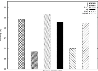
60 65 70 75 80 85 90 Accuracy (%) Feature combination L P L+O L+P P+S L+P+S
Fig. 2. The accuracies of the top six feature combinations.
and Sander [11], as listed in Table I. P consists of graph shape index (Ξ), polarizability (αp),
normal-ized Van der Waals volume (νv), hydrophobicity (Π)
and isoelectric point (I). S contains the probabilities to constitute alpha helix (α) and beta sheet (β).
In summary, the possible features included in the cysteine state classification are given as follows.
L: the local profile PSSM,
O: the order of cysteines and the normalized protein
length,
P : the five physiochemical properties, S: the structure probabilities (S).
To obtain better performance, we perform the feature selection procedure by trying all combina-tions of the four features. In other words, there are totally 16 possible feature combinations. With each of the 16 feature combinations, we employ LIBSVM package [2] to perform the classification job. Although it is a compact package, we slightly modify the codes to meet our purpose in cross
validation. That is, we do not adopt its original
“shuffle” function but use the predefined fold lists to make the comparison with the previous works in fair. Figure 2 shows the prediction accuracies of the top six feature combinations.
III. THE TUNINGMETHOD
We propose a tuning method to do slight mod-ification for the SVM output and make sure that the number of oxidized cysteines is even, since each disulfide bond is formed by a pair of oxidized
cysteines. Our tuning method changes the cysteine states with their positions and the oxidized prob-abilities from SVM output. The flow chart of our method is shown in Figure 3.
To tune up specific cysteines, we make two assumptions that the bonds or structures in Figure 4 (a) and (b) are unstable. Figure 4 (a) illustrates the situation that two oxidized cysteines on the same
β-sheet structure could not form a bond because
they are surrounded by reduced cysteines. So one predicted oxidized cysteine is assumed to not be surrounded by reduced ones.
Figure 4 (b) is another situation that the predicted state is assumed to be unstable. To make the struc-ture stable, we think that C2 should be bonded with either C4 or C5, that causes C3 or C1 to become a reduced cysteine. So our second assumption is that no reduced cysteines can be surrounded by oxidized ones.
The two assumptions form the main spirit of our algorithm for refining the initial predicted states. The tuning method is given as follows.
Algorithm: Tuning method for state classification Input: The results of SVM prediction, and the
predicted bonding probabilities. Output: The tuned result of the cysteines.
Step 1: Boundary adjustment. Check whether the cysteine is misplaced or not with the near-est neighbor method. That is, we examine the cysteine nearest to the reduced group, which we call the state transition
bound-ary. The procedure continues sequentially
until there are no error-predicted cys-teines. Take a sorted output of SVM T which is sorted by its probabilities in non-increasing order for each cysteine Ti,
1 <= i <= |T |. We first check whether the boundary j should be changed or not. If j is changed, jump to Step 2. Otherwise we will check j + 1 in the rest cysteines. Step 2: Oxidized inversion. Change the state
of each oxidized one to be reduced when it is surrounded by two or more reduced cysteines on each side.
Step 3: Reduced inversion . Change a reduced cysteine to be an oxidized one if it is sur-rounded by one or more oxidized cysteines on each side.
TABLE I
THE PHYSIOCHEMICAL PROPERTIES AND STRUCTURE PROBABILITIES OF AMINO ACIDS[15].
Amino acid One-letter Physiochemical properties (P ) Structure (S)
full-name code Ξ αp νv Π I α β Alanine A 1.28 0.05 1.00 0.31 6.11 0.42 0.23 Cysteine C 1.77 0.13 2.43 1.54 6.35 0.17 0.41 Aspartic acid D 1.60 0.11 2.78 -0.77 2.95 0.25 0.20 Glutamic acid E 1.56 0.15 3.78 -0.64 3.09 0.42 0.21 Phenylalanine F 2.94 0.29 5.89 1.79 5.67 0.30 0.38 Glycine G 0.00 0.00 0.00 0.00 6.07 0.13 0.15 Histidine H 2.99 0.23 4.66 0.13 7.69 0.27 0.30 Isoleucin I 4.19 0.19 4.00 1.80 6.04 0.30 0.45 Lysine K 1.89 0.22 4.77 -0.99 9.99 0.32 0.27 Leucine L 2.59 0.19 4.00 1.70 6.04 0.39 0.31 Methionine M 2.35 0.22 4.43 1.23 5.71 0.38 0.32 Asparagine N 1.60 0.13 2.95 -0.60 6.52 0.21 0.22 Proline P 2.67 0.00 2.72 0.72 6.80 0.13 0.34 Glutamine Q 1.56 0.18 3.95 -0.22 5.65 0.36 0.25 Arginine R 2.34 0.29 6.13 -1.01 10.74 0.36 0.25 Serine S 1.31 0.06 1.60 -0.04 5.70 0.20 0.28 Threonine T 3.03 0.11 2.60 0.26 5.60 0.21 0.36 Valine V 3.67 0.14 3.00 1.22 6.02 0.27 0.49 Tryptophan W 3.21 0.41 8.08 2.25 5.94 0.32 0.42 Tyrosine Y 2.94 0.30 6.47 0.96 5.66 0.25 0.41 P r e d i c t i o n f r o m S V M S o r t b y p r o b a b i l i t y B o u n d a r y a d j u s t m e n t S o r t b y p o s i t i o n O x i d i z e d i n v e r s i o n R e d u c e d i n v e r s i o n S o r t b y p r o b a b i l i t y O d d - e v e n r e v i s i o n O u t p u t
Fig. 3. The flow chart of the tuning method.
( a ) C 1 C3 C 4 C2 ( b ) S h e e t C 1 C3 C2 C5 C4 A A S t r u c t u r e
Fig. 4. The assumption that oxidized cysteines could not be formed into a pair, where oxidized cysteines are represented by gray nodes and the other residues are skipped by the dashed line. (a) An unstable β-sheet structure. (b) Another unstable structure.
Step 4: Odd-even revision. Adjust the number of oxidized cysteines to be even when it is odd after Step 3. This step is similar to boundary adjustment, but we check it only once. And for the future experiments, we set up an additional threshold ρ to obtain better performance.
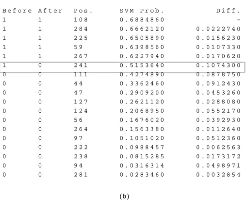
For more details, Figures 5 to 7 illustrate an example of the tuning method with a real protein (PDB ID: 1duw, chain A). Here we use 0 and 1 to represent the reduced state and oxidized state, respectively.
Figure 5 (a) shows the prediction produced by SVM with its corresponding oxidized probabilities and positions. In Step 1, we first sort the cysteines by the probabilities and then locate the cysteine at the state transition boundary, which is the oxidized cysteine with the smallest probability. We calculate the probability difference of the target cysteine by the two closest cysteines, one is oxidized and the other one is reduced, as Figure 5 (b) shows.
In this example, the cysteine at position 241 lies at the boundary where we should check its probability difference. We find that cysteine 241 is closer to the reduced group than the oxidized group. Thus, we change it to 0. In our algorithm, we then stop the adjustment and go to the next step.
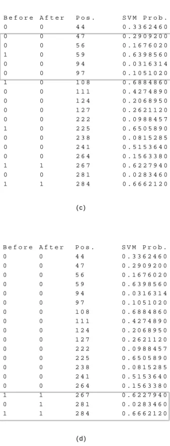
Then we check for specific cysteines depending on our two assumptions. As Figure 6 (c) shows, we perform the oxidized inversion step. We find that cysteine 59 matches our assumptions and thus turn it to be reduced. For the remaining cysteines, positions 108 and 225 also satisfy the rule and their states should be changed. After this, we perform the reduced inversion step and find that the rule is satisfied at position 281 where the cysteine state should be oxidized, as shown in Figure 6 (d).
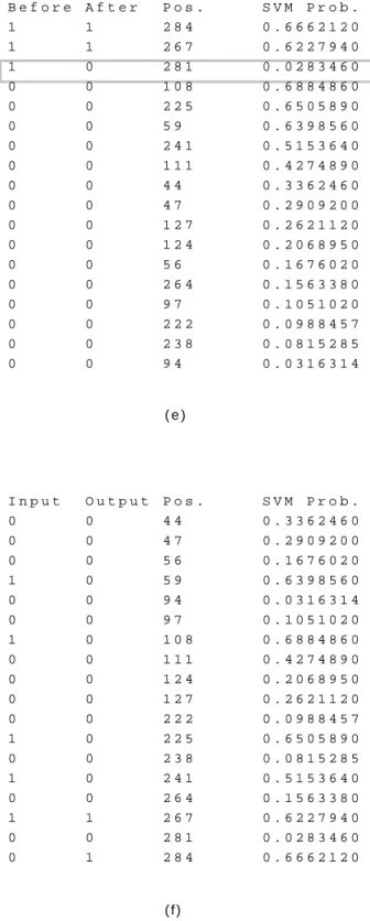
Finally, in the odd-even revision step, we check whether the total number of oxidized cysteines is even or not. Here we set a threshold ρ to refine the state adjustment. In Steps 2 and 3, we focus on the relationship between positions of cysteines and leave the probabilities out of consideration. Although the tactics help us to filter some erro-neously predicted cysteines, we also run the risk of eliminating correctly predicted ones. Consequently, in the final step, we take the most probable oxidized cysteine back according to the probability produced
by SVM.
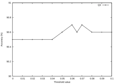
As shown in Figure 7 (e), we sort them by the states tuned in previous steps and then by probabilities which is similar to Step 1. We find the probability at position 281 is smaller than ρ; therefore we adjust the state to become reduced to make the number consistently be paired. In our experiments, as shown in Figure 8, the threshold
ρ = 0.06 can yield best results.
After finishing the above procedure, we obtain the tuned states of the sequence, as shown in Figure 7 (f). Although this strategy is simple and heuristic, it is useful.
IV. EXPERIMENTALRESULTS
A. Datasets and Performance Evaluation
To compare with the previous works, we use the same datasets as the previous works did. The PDB4136 was used by Martelli et al. [14], containing 969 proteins extracted from PDB with an identity value less than 25% and without broken chain. The dataset contains 4136 cysteines in which the number of oxidized ones is 1446. For comparison, we split it into 20 disjoint subsets and perform 20-fold cross-validation with the same list used by Martelli et al. [14].
In order to perform k-fold cross-validation for a dataset D, we split D into k disjoint subsets
D1, D2, . . . , Dk. We take one Di, 1 ≤ i ≤ k, for
testing and the other k − 1 subsets for training. This procedure repeats k times until all subsets are processed.
We also use the standard percentage accuracy as performance measurement and group the answers into 4 categories, true positive (TP), true negative (TN), false positive (FP) and false negative (FN).
For the cysteine state classification problem, the accuracy is defined as Q3 = P N = T P + T N T P + T N + F P + F N, (1)
where P denotes the total number of correct predic-tions and N denotes the number of total predicpredic-tions. For the protein-based performance, the accuracy is defined as Qp = Pp Np = T Pp+ T Np T Pp+ T Np+ F Pp+ F Np , (2)
( a ) ( b ) S V M P o s . S V M P r o b . 0 4 4 0 . 3 3 6 2 4 6 0 0 4 7 0 . 2 9 0 9 2 0 0 0 5 6 0 . 1 6 7 6 0 2 0 1 5 9 0 . 6 3 9 8 5 6 0 0 9 4 0 . 0 3 1 6 3 1 4 0 9 7 0 . 1 0 5 1 0 2 0 1 1 0 8 0 . 6 8 8 4 8 6 0 0 1 1 1 0 . 4 2 7 4 8 9 0 0 1 2 4 0 . 2 0 6 8 9 5 0 0 1 2 7 0 . 2 6 2 1 1 2 0 0 2 2 2 0 . 0 9 8 8 4 5 7 1 2 2 5 0 . 6 5 0 5 8 9 0 0 2 3 8 0 . 0 8 1 5 2 8 5 1 2 4 1 0 . 5 1 5 3 6 4 0 0 2 6 4 0 . 1 5 6 3 3 8 0 1 2 6 7 0 . 6 2 2 7 9 4 0 0 2 8 1 0 . 0 2 8 3 4 6 0 1 2 8 4 0 . 6 6 6 2 1 2 0 B e f o r e A f t e r P o s . S V M P r o b . D i f f . 1 1 1 0 8 0 . 6 8 8 4 8 6 0 -1 -1 2 8 4 0 . 6 6 6 2 -1 2 0 0 . 0 2 2 2 7 4 0 1 1 2 2 5 0 . 6 5 0 5 8 9 0 0 . 0 1 5 6 2 3 0 1 1 5 9 0 . 6 3 9 8 5 6 0 0 . 0 1 0 7 3 3 0 1 1 2 6 7 0 . 6 2 2 7 9 4 0 0 . 0 1 7 0 6 2 0 1 0 2 4 1 0 . 5 1 5 3 6 4 0 0 . 1 0 7 4 3 0 0 0 0 1 1 1 0 . 4 2 7 4 8 9 0 0 . 0 8 7 8 7 5 0 0 0 4 4 0 . 3 3 6 2 4 6 0 0 . 0 9 1 2 4 3 0 0 0 4 7 0 . 2 9 0 9 2 0 0 0 . 0 4 5 3 2 6 0 0 0 1 2 7 0 . 2 6 2 1 1 2 0 0 . 0 2 8 8 0 8 0 0 0 1 2 4 0 . 2 0 6 8 9 5 0 0 . 0 5 5 2 1 7 0 0 0 5 6 0 . 1 6 7 6 0 2 0 0 . 0 3 9 2 9 3 0 0 0 2 6 4 0 . 1 5 6 3 3 8 0 0 . 0 1 1 2 6 4 0 0 0 9 7 0 . 1 0 5 1 0 2 0 0 . 0 5 1 2 3 6 0 0 0 2 2 2 0 . 0 9 8 8 4 5 7 0 . 0 0 6 2 5 6 3 0 0 2 3 8 0 . 0 8 1 5 2 8 5 0 . 0 1 7 3 1 7 2 0 0 9 4 0 . 0 3 1 6 3 1 4 0 . 0 4 9 8 9 7 1 0 0 2 8 1 0 . 0 2 8 3 4 6 0 0 . 0 0 3 2 8 5 4
Fig. 5. An example of the tuning method. PDB ID: 1duw, chain A. (a) The input which is the output obtained from SVM. (b) The boundary adjustment step.
( c ) ( d ) B e f o r e A f t e r P o s . S V M P r o b . 0 0 4 4 0 . 3 3 6 2 4 6 0 0 0 4 7 0 . 2 9 0 9 2 0 0 0 0 5 6 0 . 1 6 7 6 0 2 0 1 0 5 9 0 . 6 3 9 8 5 6 0 0 0 9 4 0 . 0 3 1 6 3 1 4 0 0 9 7 0 . 1 0 5 1 0 2 0 1 0 1 0 8 0 . 6 8 8 4 8 6 0 0 0 1 1 1 0 . 4 2 7 4 8 9 0 0 0 1 2 4 0 . 2 0 6 8 9 5 0 0 0 1 2 7 0 . 2 6 2 1 1 2 0 0 0 2 2 2 0 . 0 9 8 8 4 5 7 1 0 2 2 5 0 . 6 5 0 5 8 9 0 0 0 2 3 8 0 . 0 8 1 5 2 8 5 0 0 2 4 1 0 . 5 1 5 3 6 4 0 0 0 2 6 4 0 . 1 5 6 3 3 8 0 1 1 2 6 7 0 . 6 2 2 7 9 4 0 0 0 2 8 1 0 . 0 2 8 3 4 6 0 1 1 2 8 4 0 . 6 6 6 2 1 2 0 B e f o r e A f t e r P o s . S V M P r o b . 0 0 4 4 0 . 3 3 6 2 4 6 0 0 0 4 7 0 . 2 9 0 9 2 0 0 0 0 5 6 0 . 1 6 7 6 0 2 0 0 0 5 9 0 . 6 3 9 8 5 6 0 0 0 9 4 0 . 0 3 1 6 3 1 4 0 0 9 7 0 . 1 0 5 1 0 2 0 0 0 1 0 8 0 . 6 8 8 4 8 6 0 0 0 1 1 1 0 . 4 2 7 4 8 9 0 0 0 1 2 4 0 . 2 0 6 8 9 5 0 0 0 1 2 7 0 . 2 6 2 1 1 2 0 0 0 2 2 2 0 . 0 9 8 8 4 5 7 0 0 2 2 5 0 . 6 5 0 5 8 9 0 0 0 2 3 8 0 . 0 8 1 5 2 8 5 0 0 2 4 1 0 . 5 1 5 3 6 4 0 0 0 2 6 4 0 . 1 5 6 3 3 8 0 1 1 2 6 7 0 . 6 2 2 7 9 4 0 0 1 2 8 1 0 . 0 2 8 3 4 6 0 1 1 2 8 4 0 . 6 6 6 2 1 2 0
Fig. 6. An example of the tuning method. PDB ID: 1duw, chain A (continued). (c) The oxidized inversion step. (d) The reduced inversion step.
( e ) ( f ) B e f o r e A f t e r P o s . S V M P r o b . 1 1 2 8 4 0 . 6 6 6 2 1 2 0 1 1 2 6 7 0 . 6 2 2 7 9 4 0 1 0 2 8 1 0 . 0 2 8 3 4 6 0 0 0 1 0 8 0 . 6 8 8 4 8 6 0 0 0 2 2 5 0 . 6 5 0 5 8 9 0 0 0 5 9 0 . 6 3 9 8 5 6 0 0 0 2 4 1 0 . 5 1 5 3 6 4 0 0 0 1 1 1 0 . 4 2 7 4 8 9 0 0 0 4 4 0 . 3 3 6 2 4 6 0 0 0 4 7 0 . 2 9 0 9 2 0 0 0 0 1 2 7 0 . 2 6 2 1 1 2 0 0 0 1 2 4 0 . 2 0 6 8 9 5 0 0 0 5 6 0 . 1 6 7 6 0 2 0 0 0 2 6 4 0 . 1 5 6 3 3 8 0 0 0 9 7 0 . 1 0 5 1 0 2 0 0 0 2 2 2 0 . 0 9 8 8 4 5 7 0 0 2 3 8 0 . 0 8 1 5 2 8 5 0 0 9 4 0 . 0 3 1 6 3 1 4 I n p u t O u t p u t P o s . S V M P r o b . 0 0 4 4 0 . 3 3 6 2 4 6 0 0 0 4 7 0 . 2 9 0 9 2 0 0 0 0 5 6 0 . 1 6 7 6 0 2 0 1 0 5 9 0 . 6 3 9 8 5 6 0 0 0 9 4 0 . 0 3 1 6 3 1 4 0 0 9 7 0 . 1 0 5 1 0 2 0 1 0 1 0 8 0 . 6 8 8 4 8 6 0 0 0 1 1 1 0 . 4 2 7 4 8 9 0 0 0 1 2 4 0 . 2 0 6 8 9 5 0 0 0 1 2 7 0 . 2 6 2 1 1 2 0 0 0 2 2 2 0 . 0 9 8 8 4 5 7 1 0 2 2 5 0 . 6 5 0 5 8 9 0 0 0 2 3 8 0 . 0 8 1 5 2 8 5 1 0 2 4 1 0 . 5 1 5 3 6 4 0 0 0 2 6 4 0 . 1 5 6 3 3 8 0 1 1 2 6 7 0 . 6 2 2 7 9 4 0 0 0 2 8 1 0 . 0 2 8 3 4 6 0 0 1 2 8 4 0 . 6 6 6 2 1 2 0
90 90.2 90.4 90.6 90.8 91 0 0.01 0.02 0.03 0.04 0.05 0.06 0.07 0.08 0.09 0.1 Accuracy (%) Threshold value Q3
Fig. 8. Accuracies of various values of threshold ρ in the tuneing method.
where Pp is the correct predictions of proteins and
Np is total number of proteins in the testing set.
In order to make the cross-validation fair, all the statistics are calculated with the same parameters,
cost (C) and gamma (γ), for SVM. For example,
suppose there are 3 sets of parameters, (C1, γ1), (C2, γ2) and (C3, γ3) in a window size w. The accuracy for this window size is defined as the maximum one of Q(C1,γ1), Q(C2,γ2) and Q(C3,γ3).
Moreover, we also consider the commonly used indexes such as sensitivity, specificity and Matthews
correlation coefficients (MCC), which are defined
as follows. Specif icity = T N T N + F P. (3) Sensitivity = T P T P + F N. (4) M CC =√ T P× T N − F P × F N (T P + F N )(T P + F P )(T N + F P )(T N + F N ) . (5) B. Experimental Results
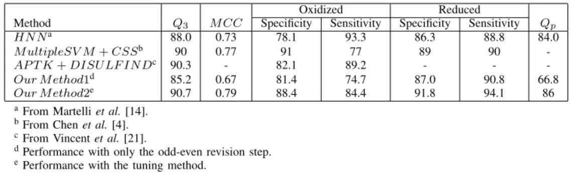
Table II shows the accuracy comparison between our tuning method and previous works. As we can see, the best result in previous works is the method of Vincent et al.[21]. They constructed a kernel-based SVM method, all-pairs decomposition
kernel (APDK), to solve the problems of chain
classification, state classification and connectivity prediction.
In Table II, “Our Method1” adopts only the odd-even revision step. In other words, “Our Method1”
only makes the number of oxidized cysteines even after the prediction of SVM. On the other hand, “Our Method2” adopts the whole steps of the tuning method with threshold rho to make the modification more precisely. We find Qp and Q3 are improved after the whole tuning method is executed.
In our method, the boundary adjustment step first reduces the risk when the data are ambiguous for SVM. And with the specific target revision, we take back and throw away the cysteines of wrong prediction by its positions in the sequence. The steps make up the defects of SVM, in which the model will be affected by distributions of samples in the training set.
For various window sizes, the accuracies are shown in Table III. In this table, we find that there is a tendency between window sizes and accuracies. Although the window approach is based on the idea that the information beside the target cysteine is useful, it also makes it indistinct for SVM. Take Q3 as an example, the accuracies increase till the 25-residue window and then decrease. This phenomenon implies that there is no global rule to decide the window size.
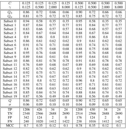
The details of the best result are shown in Tables IV and V. In this dataset, the best performance is on a 25-residue window with SVM parameters C = 2.0 and γ = 0.125 where we achieve Qc = 90.7%
and Qp = 86%. Moreover, the standard deviation
σ = 0.03 means that our method is stable in the
TABLE II
ACCURACY COMPARISON FORPDB4136DATASET.
Oxidized Reduced
Method Q3 M CC Specificity Sensitivity Specificity Sensitivity Qp
HN Na 88.0 0.73 78.1 93.3 86.3 88.8 84.0
M ultipleSV M + CSSb 90 0.77 91 77 89 90
-AP T K + DISU LF IN Dc 90.3 - 82.1 89.2 - -
-Our M ethod1d 85.2 0.67 81.4 74.7 87.0 90.8 66.8
Our M ethod2e 90.7 0.79 88.4 84.4 91.8 94.1 86 aFrom Martelli et al. [14].
bFrom Chen et al. [4]. cFrom Vincent et al. [21].
dPerformance with only the odd-even revision step. ePerformance with the tuning method.
TABLE III
ACCURACIES OFPDB4136DATASET FOR VARIOUS WINDOW SIZES WITH20-FOLD CROSS-VALIDATION.
Window Oxidized Reduced
size Q3 M CC Specificity Sensitivity Specificity Sensitivity Qp
7 88.2 0.74 84.5 81.3 90.2 92.0 82.6 9 88.9 0.75 85.9 81.7 90.4 92.8 84.4 11 89.0 0.76 85.6 82.3 90.7 92.6 84.2 13 89.0 0.76 85.1 83.0 91.0 92.2 84.4 15 89.3 0.76 85.9 83.1 91.1 92.6 84.9 17 89.1 0.76 85.6 82.7 90.9 92.5 84.5 19 89.7 0.77 86.6 83.3 91.2 93.1 85.0 21 89.7 0.77 87.5 82.2 90.7 93.7 85.6 23 89.9 0.78 87.2 83.5 91.3 93.4 85.3 25 90.7 0.79 88.4 84.4 91.8 94.1 86.0 27 89.9 0.78 86.6 84.2 91.6 93.0 84.9 29 89.6 0.77 86.8 82.7 90.9 93.2 84.8 31 89.3 0.76 86.6 82.0 90.6 93.2 84.9 33 88.5 0.75 85.7 80.7 89.9 92.8 84.5 V. CONCLUSIONS
In this paper, we propose a tuning method for refining the predicted cysteine state obtained from SVM. Experimental results reveal that higher ac-curacies are achieved compared with the previous works. Although we believe this strategy can be used in other situations, even to tune up the results of previous works, we also realize its limitation. First, our method is recommended when there are more than four cysteines in a protein. Second, our method is devised to add the lost ones but still lacks mechanism for deletion when there is an error prediction.
We show that the problem can be solved by simple but logic rules. With the sequence profile and window approach as a local view, we can predict the state of each cysteines. And with our tuning method, we can improve the accuracy by about 20% in Qp
and 5% in Q3. The result is better than the previous works.
REFERENCES
[1] S. F. Altschul, T. L. Madden, A. A. Schaffer, J. Zhang, Z. Zhang, W. Miller, and D. J. Lipman, “Gapped blast and psi-blast: a new generation of protein database search programs,”
Nucleic Acids Research, Vol. 25, No. 17, pp. 3389–3402, 1997.
[2] C.-C. Chang and C.-J. Lin, “LIBSVM: a library for support vector machines,” 2001. Software available at http://www.csie. ntu.edu.tw/∼cjlin/libsvm.
[3] G. Chen, H. Deng, Y. Gui, Y. Pan, and X. Wang, “Cysteine sep-arations profiles on protein secondary structure infer disulfide connectivity,” Granular Computing, 2006 IEEE International
Conference on, pp. 663–665, May 2006.
[4] Y.-C. Chen, Y.-S. Lin, C.-J. Lin, and J.-K. Hwang, “Prediction of the bonding states of cysteines using the support vector machines based on multiple feature vectors and cysteine state sequences,” PROTEINS: Structure, Function, and Genetics, Vol. 55, pp. 1036–1042, 2004.
[5] C.-C. Chuang, C.-Y. Chen, J.-M. Yang, P.-C. Lyu, and J.-K. Hwang, “Relationship between protein structures and disulfide-bonding patterns,” PROTEINS: Structure, Function, and
Genet-ics, Vol. 53, pp. 1–5, 2003.
[6] P. Fariselli, P. Riccobelli, and R. Casadio, “Role of evolutionary information in predicting the disulfide-bonding state of cysteine in proteins,” PROTEINS: Structure, Function, and Genetics, Vol. 36, pp. 340–346, 1999.
TABLE IV
THE DETAILED ACCURACIES OF ALL SUBSETS INPDB4136WITH VARIOUS VALUES OFCANDγ,AND FIXED WINDOW SIZE25.
C 0.125 0.125 0.125 0.125 0.500 0.500 0.500 0.500 γ 0.125 0.500 2.000 8.000 0.125 0.500 2.000 8.000 Q3 0.86 0.72 0.66 0.66 0.90 0.72 0.66 0.66 Qp 0.81 0.75 0.72 0.72 0.85 0.75 0.72 0.72 Subset 0 0.94 0.58 0.35 0.35 0.95 0.58 0.35 0.35 Subset 1 0.87 0.84 0.77 0.77 0.91 0.84 0.77 0.77 Subset 2 0.83 0.66 0.57 0.57 0.84 0.68 0.57 0.57 Subset 3 0.84 0.67 0.64 0.64 0.88 0.67 0.64 0.64 Subset 4 0.9 0.86 0.8 0.81 0.93 0.86 0.8 0.81 Subset 5 0.86 0.61 0.62 0.62 0.9 0.61 0.62 0.62 Subset 6 0.91 0.74 0.71 0.68 0.93 0.74 0.71 0.68 Subset 7 0.8 0.75 0.68 0.68 0.88 0.75 0.68 0.68 Subset 8 0.95 0.76 0.68 0.68 0.95 0.76 0.68 0.68 Subset 9 0.89 0.64 0.61 0.6 0.89 0.64 0.61 0.6 Subset 10 0.86 0.81 0.78 0.78 0.91 0.81 0.78 0.78 Subset 11 0.76 0.69 0.68 0.67 0.89 0.69 0.68 0.67 Subset 12 0.82 0.74 0.62 0.62 0.9 0.74 0.62 0.62 Subset 13 0.92 0.75 0.71 0.71 0.93 0.75 0.71 0.71 Subset 14 0.77 0.74 0.67 0.67 0.85 0.74 0.67 0.67 Subset 15 0.84 0.8 0.72 0.72 0.96 0.8 0.72 0.72 Subset 16 0.93 0.71 0.61 0.61 0.97 0.71 0.61 0.61 Subset 17 0.78 0.68 0.63 0.63 0.82 0.68 0.63 0.63 Subset 18 0.85 0.84 0.74 0.74 0.88 0.84 0.74 0.74 Subset 19 0.87 0.56 0.49 0.49 0.88 0.56 0.49 0.49 Q 0.86 0.72 0.65 0.65 0.90 0.72 0.65 0.65 σ 0.06 0.09 0.10 0.10 0.04 0.09 0.10 0.10 TP 1206 426 34 24 1208 430 34 24 TN 2348 2566 2688 2690 2514 2566 2688 2690 FP 342 124 2 0 176 124 2 0 FN 240 1020 1412 1422 238 1016 1412 1422 MCC 0.7 0.35 0.12 0.1 0.78 0.35 0.12 0.1
[7] F. Ferre and P. Clote, “Disulfide connectivity prediction using secondary structure information and diresidue frequencies,”
Bioinformatics, Vol. 21, No. 10, pp. 2336–2346, 2005.
[8] A. Fiser and I. Simon, “Predicting the oxidation state of cys-teines by multiple sequence alignment,” Bioinformatics, Vol. 16, No. 3, pp. 251–256, 2000.
[9] P. Frasconi, A. Passerini, and A. Vullo, “A two-stage svm archi-tecture for predicting the disulfide bonding state of cysteines,”
Neural Networks for Signal Processing, 2002. Proceedings of the 2002 12th IEEE Workshop on, pp. 25–34, 2002.
[10] P. M. Harrison and M. J. E. Sternberg, “Analysis and clas-sification of disulphide connectivity in proteins : The entropic effect of cross-linkage,” Journal of Molecular Biology, Vol. 244, No. 4, pp. 448–463, 1994.
[11] L. Holm and C. Sander, “Mapping the protein universe,”
Science, Vol. 273, No. 5275, pp. 595–602, 1996.
[12] D. T. Jones, “Protein secondary structure prediction based on position-specific scoring matrices,” Journal of Molecular
Biology, Vol. 292, No. 2, pp. 195–202, 1999.
[13] C.-H. Lu, Y.-C. Chen, C.-S. Yu, and J.-K. Hwang, “Predicting disulfide connectivity patterns,” PROTEINS: Structure,
Func-tion, and Genetics, Vol. 67, pp. 262–270, 2007.
[14] P. L. Martelli, P. Fariselli, L. Malaguti, and R. Casadio, “Pre-diction of the disulfide-bonding state of cysteines in proteins at 88% accuracy,” Protein Science, Vol. 11, pp. 2735–2739, 2002. [15] J. Meiler, M. Muller, A. Zeidler, and F. Schmaschke, “Genera-tion and evalua“Genera-tion of dimension-reduced amino acid parameter representations by artificial neural networks,” Journal of
Molec-ular Modeling, Vol. 7, pp. 360–369, 2001.
[16] L. A. Mirny and E. I. Shakhnovich, “How to derive a protein folding potential? a new approach to an old problem,” Journal
of Molecular Biology, Vol. 264, No. 5, pp. 1164–1179, 1996.
[17] S. M.Muskal, S. R.Holbrook, and S.-H. Kim, “Prediction of the disulfide-bonding state of cysteine in proteins,” Protein
Engineering, Vol. 3, No. 8, pp. 667–672, 1990.
[18] M. Mucchielli-Giorgi, S. Hazout, and P. Tuffery, “Predicting the disulfide bonding state of cysteines using protein descrip-tors,” PROTEINS: Structure, Function, and Genetics, Vol. 46, pp. 243–249, 2002.
[19] R. Rubinstein and A. Fiser, “Predicting disulfide bond connec-tivity in proteins by correlated mutations analysis,”
Bioinfor-matics, Vol. 24, No. 4, pp. 498–504, 2008.
[20] R. Singh, “A review of algorithmic techniques for disulfide-bond determination,” Brief Funct Genomic Proteomic, Vol. 7, No. 2, pp. 157–172, 2008.
[21] M. Vincent, A. Passerini, M. Labbe, and P. Frasconi, “A simplified approach to disulfide connectivity prediction from protein sequences,” BMC Bioinformatics, Vol. 9, No. 1, p. 20, 2008.
TABLE V
THE DETAILED ACCURACIES OF ALL SUBSETS INPDB4136WITH VARIOUS VALUES OFCANDγ,AND FIXED WINDOW SIZE25
(CONTINUED). C 2.000 2.000 2.000 2.000 8.000 8.000 8.000 8.000 γ 0.125 0.500 2.000 8.000 0.125 0.500 2.000 8.000 Q3 0.91 0.76 0.66 0.66 0.90 0.76 0.66 0.66 Qp 0.86 0.77 0.72 0.72 0.85 0.77 0.72 0.72 Subset 0 0.92 0.58 0.35 0.35 0.94 0.58 0.35 0.35 Subset 1 0.92 0.86 0.77 0.77 0.89 0.86 0.77 0.77 Subset 2 0.85 0.81 0.57 0.57 0.86 0.81 0.57 0.57 Subset 3 0.9 0.73 0.64 0.64 0.9 0.73 0.64 0.64 Subset 4 0.93 0.83 0.8 0.81 0.92 0.83 0.8 0.81 Subset 5 0.95 0.73 0.62 0.62 0.96 0.73 0.62 0.62 Subset 6 0.91 0.74 0.71 0.68 0.91 0.74 0.71 0.68 Subset 7 0.89 0.78 0.68 0.68 0.89 0.78 0.68 0.68 Subset 8 0.95 0.79 0.68 0.68 0.95 0.79 0.68 0.68 Subset 9 0.92 0.68 0.61 0.6 0.92 0.68 0.61 0.6 Subset 10 0.92 0.88 0.78 0.78 0.91 0.88 0.78 0.78 Subset 11 0.9 0.72 0.68 0.67 0.88 0.72 0.68 0.67 Subset 12 0.88 0.77 0.62 0.62 0.88 0.77 0.62 0.62 Subset 13 0.91 0.8 0.71 0.71 0.92 0.8 0.71 0.71 Subset 14 0.9 0.76 0.67 0.67 0.84 0.76 0.67 0.67 Subset 15 0.96 0.76 0.72 0.72 0.93 0.76 0.72 0.72 Subset 16 0.96 0.76 0.61 0.61 0.95 0.76 0.61 0.61 Subset 17 0.84 0.71 0.63 0.63 0.84 0.71 0.63 0.63 Subset 18 0.88 0.87 0.74 0.74 0.88 0.87 0.74 0.74 Subset 19 0.86 0.65 0.49 0.49 0.86 0.65 0.49 0.49 Q 0.91 0.76 0.65 0.65 0.90 0.76 0.65 0.65 σ 0.03 0.07 0.10 0.10 0.04 0.07 0.10 0.10 TP 1220 557 34 24 1212 557 34 24 TN 2530 2591 2688 2690 2514 2591 2688 2690 FP 160 99 2 0 176 99 2 0 FN 226 889 1412 1422 234 889 1412 1422 MCC 0.79 0.45 0.12 0.1 0.78 0.45 0.12 0.1