Journal of
Materials
P r o c e s s i n g T e c h n o l o g y E L S E V I E R Journal of Materials Processing Technology 47 (1995) 231-249
Analysis of cutting forces in ball-end milling
S h i u h - T a r n g C h i a n g , C h u n g - M i n Tsai, A n - C h e n Lee*Department o[" Mechanical Engineering, National Chiao Tung Unit:ersity, 1001 Ta Hsueh Road. Hsinehu 30049, Taiwan
(Received June 8, 1993)
Industrial Summary
A cutting force model for ball end milling is developed, the model being based mainly on the assumption that the cutting force is equal to the product of the cutting area and the specific cutting force. The formulation of the cutting area is derived from the geometry of the mill and the workpiece, whilst the specific cutting force is obtained by third-order curve-fitting of data measured in experiments. The model established in this paper predicts the cutting forces in ball-end milling much more accurately than do previous models.
1. Introduction
Ball-end milling plays an important role in three-dimensional machining, because it has the ability to machine three-dimensional curves easily. While a curved surface is being milled, the tangential cutting speed is minimum (equal to zero) at the tip of the ball, since the rotating radius there is zero, and it is at its maximum value at the periphery of the ball-end mill. When the speed varies along the cutting edge, the related cutting force also changes along the three-dimensional cutting edge. Ball-end milling is thus unlike end milling or face milling, in which the force occurs at the cylindrical periphery of the mill, and it is much more difficult to analyze the force variation in ball-end milling than in these other types of milling. The goal of the present research is to establish a force model to elucidate ball-end milling.
Several studies of end milling have been published [1-3], but studies of ball end milling are few. For the case of full milling, in 1988 Fujii et al. [4] developed a cutting-force model of ball-end milling based on the relationship between the cutting
* Corresponding author.
0924-0136/95/$09.50 (C~ 1995 Elsevier Science S.A. All rights reserved SSDI 0 9 2 4 - 0 1 3 6 ( 9 5 ) 0 1 3 2 5 - U
232 S.-T. Chiang et al. / Journal of Materials Processing Technology 47 (1995) 231 249 area and the specific cutting force, other cases, such as different radial depths of cut and an axial depth of cut greater than the radius of the mill, being left out of their account. In 1991, Yang and Park [-5] also presented a cutting-force model of ball-end milling, in their paper the cutting-force model being based on the fundamental mechanics of orthogonal cutting, which assumes that the shear angle, shear stress, and friction angle are functions of cutting speed, feedrate, and normal rake angle, the values of these former three parameters being obtained from turning experiments. However, Yang and Park's theoretical and experimental results do not match very well, because there is a large difference in chip formulation, shear angle, and friction angle between ball-end milling and turning. Hirota and Usui [6] pointed out that the energy dissipation within the chip could not be ignored in larger helix angle cutting, therefore using orthogonal-cutting mechanics to analyze ball-end milling is questionable.
To compensate for the defects of existing models, a new force model is proposed in this paper. In Section 2, a simple and accurate formulation of cutting geometry is proposed based on the method in [4]. In Section 3, a cutting-area model that includes all cutting conditions is developed and a method is presented for calculating the cutting forces of both the ball part and the end-mill part in ball end milling: in the latter operation, not only the ball part but also the end-mill part can machine the workpiece. Existing models deal only with the ball part of ball-end milling, whereas the two parts of the cutter are considered in the present work. Further- more, in the present work the force model is by considering the effect of the cusp on the workpiece. In end milling, the effect of the cusp is insignificant, but in ball- end milling it is serious. In Section 4, a cutting-force model is proposed based on the product of the cutting area and the specific cutting force, in this model the effect of workpiece hardness being considered: From the point of view of force prediction, it is necessary to study this effect. Finally, in Section 5, a series of experiments performed using various cutting conditions is described, the experimental results for cutting forces verifying the proposed model and showing that it provides consistent results.
2. The cutting edge geometry
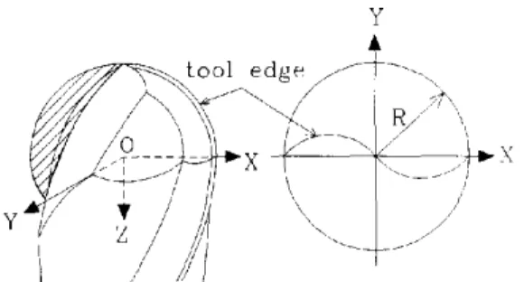
2.1. The cutting edge profileThe shape of the edge will affect the outline of the cutting area, i.e. it will affect the cutting force, therefore a full analysis of the silhouette of the edge is the starting point in modeling the cutting-force model. The type of mill studied in this paper is a right-hand screw ball-end mill manufactured by the Nachi Co., the nominal radius of the ball-end mill, the length of the mill, the length of the edge, and the helix angle being 8 mm, 140 mm, 40 mm, and 30 °, respectively.
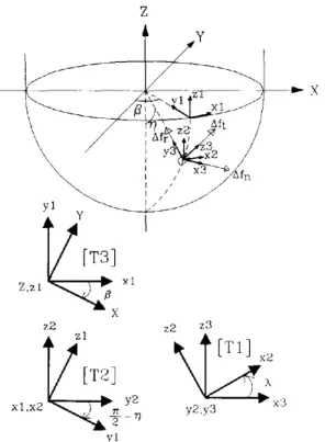
To represent the outline of the edge by a function of coordinates x, y, and z, the origin is defined as being at the center of the ball-end mill. The directions of X, Y, and Z are plotted in Fig. 1. The outline of the edge can be approximated by the
S.-T. Chiang et al. / Journal O/" Materials Process#1g Technology 47 (1995) 231.-249 Y
L o o l e d g e \
Fig. 1. Cutter geometry and coordinate system for down ball-end milling.
233
following equations: x
=f(t)=
Rty = ,q(t) = - R ( a l t4 + a2 t3 + a3 t2 + a4t + as),
(l)
z = h(t) = - R ( b t t 4 + b2 t3 + b3 t2 + b4t + bs) 1/2,where R is the nominal radius of the ball nose, t is a parameter that satisfies 0 ~< t ~< 1, and al a5 and b l - b s are constant parameters.
The profile of the edge was measured using a three-dimensional coordinate- measurement machine, the measured data being applied in Eq. (1) and the least- squares method employed to obtain the ten constant parameters listed in Table 1.
2.2. H e l i x angle a n d phase d(fferenee
The cutting area is located in the contacting position between the edge and workpiece, but the contacting position depends on the phase difference and the helix angle of the above edge position. Therefore, the phase difference and helix angle must be defined clearly in order to be able to derive the cutting area.
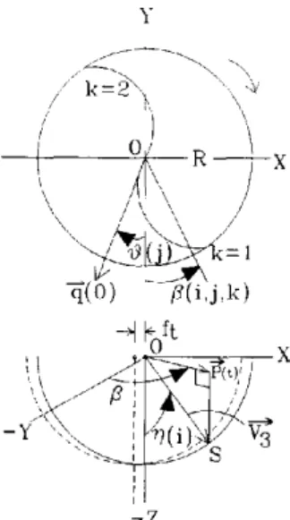
The definition of phase difference ~ is shown in Fig. 2(a). The tangential vector on the top of the ball end (t = 0) projected on the O - X - Y plane is defined as q(0), which can be written as (f'(0), 9'(0), 0), where the prime denotes the derivation with respect to parameter t. The line from the top point to any position S of the edge projected on to the O - X Yplane is defined asp(t), which is written as (f(t),9(t),O). The angle between q(0) aud p(t) is the phase difference ~ of the point S. Thus the phase difference ~ can be derived by the dot product of q(0) and p(t) or
= , (p(t). q(O)
cos \ l p ~ t Iq(~-I/
( f ( t ) f ' ( O ) 4-_ ,q(t)g'(O) c o s - 1\v/f(t)2
+ g(t) 2 ~ f ' ( o t 2 + g'(o)2 / "(2)
234 S.-T. Chiang et al. / Journal of Materials' Processing Technology 47 (1995) 231 249
Table 1
Coefficients of the edge profile
a 1 = - 0.73517 b t = - 0.54104 a 2 = 0.99551 b e = 1.363339 a3= -0.83028 b3= - 1.88824 a 4 = 0.63169 b 4 = 0.14032 a s = - 0.00494 b 5 = 1.00017 a
(-g,f,O)
A r e a A 1~
V l = ( f ' , g ' , h ' )Vz
Fig. 2. The definition of phase difference ct and helix angle and the relationship between the infinitesimal cutting area A~ and A.
T h e d e f i n i t i o n of t h e helix a n g l e 2 is g i v e n in Fig. 2(b), b e i n g t h e a n g l e b e t w e e n the t a n g e n t i a l line o f t h e p o i n t S a n d t h e vertical p l a n e , w h i c h is f o r m e d b y t h e p o i n t S a n d t h e c e n t r a l axis of t h e mill. As s h o w n in Fig. 2(a), v e c t o r V1 is the v e c t o r of t h e t a n g e n t i a l line of S a n d v e c t o r V2 is t h e n o r m a l v e c t o r of p(t) in t h e O - X - Y p l a n e . T h u s t h e helix a n g l e c a n be d e t e r m i n e d b y t h e d o t p r o d u c t of t h e v e c t o r s I"1 a n d V2.
v,
vz
c o s ( ~ - 2 ) = ' v ,
~''/11 v2l'
(3)
,~ = ~--COS 1 ( ~ f
--f'(t)g(t)+f(t)g'(t)
)
( t ) 2 +g(t) 2 x/f'(/) 2
+g'(t) 2 + h'(t) 2 "
(4)
T h e v a l u e s of t h e p h a s e difference ~ a n d helix 2 a n g l e c a n be c a l c u l a t e d b y s e t t i n g the v a l u e of t in Eqs. (2) a n d (4).S.-T. Chiang et al. / Journal o/Materials Processing Technology 47 (1995) 231- 249 235
3. Procedures for deriving the cutting area
The cutting area is defined as the product of the chip thickness and the depth of cut. Because the cutting chip thickness is generated by the three dimensional curve of the cutting edge, it is difficult, for example, to determine on what cutting plane it lies, let alone for it to directly represent the cutting area. Therefore, an approximation method is applied that divides the cutting edge into infinitesimal sections. For each section, the related chip thickness and depth of cut are calculated to obtain the cutting area, and then this is substituted into the force model to obtain the infinitesimal cutting force. Finally, the infinitesimal forces are accumulated to obtain the total force.
3.1. The infinitesimal area o f the cutting edge on the ball part
The ball-end mill comprises the ball part and the end-mill part. In the ball part, the cutting edge is located on a spherical surface whilst in the end mill part, the edge is located on a cylindric surface. Since the edge shapes of the two parts are different, their cutting behavior and paths are different. In this section is presented a method of calculating the infinitesimal area of the cutting area on the ball part. The following definitions of angles 0, q, and fl on the ball end-mill are illustrated in Fig. 3: 0, the angular position of the cutter, is the angle between the vector q(0) and the negative Y axis, the clockwise rotation being defined as positive, q is the angle between the vector V3 from the origin to the point S and the central axis (-Z) of the mill, the value of q being equal to sin l(t). fl, the engage angle, is the angle between the vector p(t) and the negative Y axis, the counterclockwise rotation being defined as positive.
/ k =2 ,~ ,,
/
5(0) F~(i;j,k)
•Oft
/
236 S.-T. Chiang et al. / Journal of Materials Processing Technology 47 (1995) 231 249 In order to describe adequately the position of the infinitesimal cutting area, q is discretized into a small section At/, whether the ith incremental angle q(i) equals i A~/, and the total number of sections is Ni. 0 is divided into N j analytical points per cycle, thus thejth rotating angle O(j) isj (2re~N j). For a mill with two teeth, the angle between the two teeth is rr radians.
The angle fl characterizes completely the position of the cutting edge at any given instant. For the right-hand helix mill, c~ and fl have the same direction, therefore the engage angle f l ( i , j , k ) c a n be written as
f l ( i , j , k ) = - O(j) + ¢t(i) + rt(k - 1), (5)
where ~(i) can be derived by inserting a given value of t, where t = sin q(i), into Eq. (2). The chip thicknes and cutting area are now expressed with respect to the fixed frame O - X - Y - Z . A simple chip-thickness formulation [1] for milling is f, sin fl, were f, is the feedrate per tooth. In the down ball-end milling shown in Fig. 3, the chip-thickness formulation should be modified. A chip thickness tc along the q direc- tion for thejth rotating angle and the ith infinitesimal cutting area of the kth tooth can be written as
tc(i,j, k) = f sin fl(i,j, k) sin r/(i), (6)
where r/(i) = izXr/. If Aq is very small, the infinitesimal cutting area projected on the vertical plane can be written as
A l ( i , j , k ) = t c ( i , j , k ) R z X q = f s i n f l ( i , j , k ) s i n q ( i ) R A q . (7) If the effect of helix angle )~ is considered, the A1 obtained has an angle ), with the actual cutting area, as shown in Fig. 2(b). Thus the infinitesimal cutting area A is modified to
A ( i , j , k ) = A ~ ( i , j , k ) s e c ) ~ ( i )
= f sin fl(i,j, k) sin r/(i) R Aq sec )~(i), (8) where ).(i) can be derived by inserting a given value of t into Eq. (4). From Eq. (8), the cutting area increases with parameter )., i.e., the cutting force for a larger value of angle ~1 is greater than that for a smaller value.
3.2. The infinitesimal cutting area on the end-mill part
If the axial depth of cut Ad is deeper than the ball part, that is Aa/> R, Eq. (8) is no longer applicable. To incorporate the effect of the end-mill part, the concept construc- ted by Kline [3] is employed to obtain the infinitesimal cutting area for end milling. In the end-mill part, the phase difference c~ in Eq. (5) is modified to
~(i) = ~o + :~e(i), (9)
where: ~o is the phase difference caused by the ball part, which can be obtained by letting t = 1 in Eq. (2); and :~e is the phase difference caused by the end-mill part.
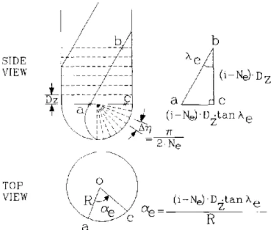
S.-T. Chiang et al. / Journal ~?f Materials Processing Technology 47 (1995) 231-.249 237 Ne is defined as the number of infinitesimal cutting areas of the ball part, in which Ne equals ~/(2 At/), the total number of areas for the ball part and end-mill part being N~. If the ith calculating infinitesimal element, Ne < i < N;, is considered, the infini- tesimal cutting area is on the end-mill part. The phase difference ~ is illustrated in Fig. 4. The ~e(i) of the ith disk can be represented in the form
( i - Ne)D= tan 2e
~(i) = , (10)
R
where Dz is the unit height along the Z axis and 2e is a constant of the helix angle of the end-mill part.
From Eq. (9) the new phase angle ~ is substituted into Eq. (5), and the new engage angle fl obtained. The infinitesimal cutting area projected onto the vertical cross- section is determined easily as f sin fi D~. Because the end-mill part has a constant helix angle )~e, the actual infinitesimal cutting area on the end mill part is described by
A (i,j, k) = f sin fl(i,j, k) D= sec 3,~. (1 l) Eq. (11) is an improved model that has less error than that presented by Kline [3]. The term sec 3o~ in Eq. (11) can fit the slope of the edge exactly, thus making the present model more precise than Kline's, which approximates the slope of an edge by a saw-tooth.
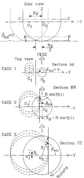
3.3. Cutting range and cusp e/~'ct
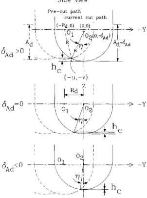
The parameters influencing the cutting range of ball-end milling are the axial depth of cut Ad, the radial depth of cut Rd, and the cusps on the workpiece. From Fig. 5, Ol is an adjacent center of the pre-cut path and 02 is the current path center with some variation of axial depth of cut 3Ao. In plane cutting, 6Ad is zero, whilst in curvature surface cutting 3Ad is either positive or negative. If it is assumed that the current
SIDE VIEW TOP V I E W
/o-h
a b~
(i Ne).D Z C (i-Ne) "Dztan X e - 2 . N e ~ _ (i-Ne)'D7~tan ;ke R238 S.-T. Chiang et al. / Journal of Materials Processing Technology 47 (1995) 231 249 d
%d=o
SAd 0
Side view i Pre-cut path ] LI I cu . . . . t cut path I - a -I / (-Rd,0) ( 0 0 ) ] L T , - ; - -- - - v - - - ' . . . . ---> - Y',,,
A d \\ ~ R VT]~// /Ad+~SAdh ? \ i
(-u,-v/
-J?-<?~~~!/h¢
. . . - > - Yi
__oli .... ÷
4 o,
_,
__iS~ho
Fig. 5. The cusp height h, related to variation of depth of cut 6Ad.
position of center 02 with zero 6,~, is at the original c o o r d i n a t e (0, 0), the intersection point ( - u, - v) is the engage line of the current t o o t h intersected with one of the past cuts. T h e values of u and v can be o b t a i n e d from the following relationship:
(-- u-F Rd) 2 + /;2 = R 2,
U 2 "F (-- U "4- t~Ad) 2 = R 2. (12)
After the a b o v e e q u a t i o n is solved, the current cusp height hc can be described as follows:
hc = R 6A~ Rd / 4 R 2 - R 2 - 62a~
T h e value hc increases when 6Ao goes f r o m positive to negative. T h e cutting range can be determined accurately by using the value of hc. Consider the engage angle f in any horizontal cross-section. T h e cutting range of f is b o u n d e d by the exit angle flex and entry angle fe., i.e.,
S.-T. Chiang et al. / Journal o/ Materials Processing Technology 47 (1995) 231 249 239 As described in Fig. 5, it is obvious that if the cutting area is below the cusp height he, the cutting process is full milling. In this situation, the entry angle fie. is ~ and the exit angle flex is zero. When the cutting area is above the cusp height, the value of flex still equals zero, but the value of fie, changes. The formulation of flen can be obtained for various values of tl(i), i.e., the height of the cutting area, using the following equations:
fien = n, case 1, if R(1 - cos q(i)) < hc --cos t 1 Rs~nq(i) ' case2, i f h c < ~ R ( l - c o s q ( i ) ) < R
= cos_l ( 1 _ ~__da), case 3, ifR~< R ( 1 - cosq(i)). (15) Fig. 6 shows the three cases of Be° with respect to values of R(1 - cosq(i)) with zero 6A~. In case 1, R(1 -- cos q(i)) is smaller than he, which means that the cusp is being formed, and fle~ equals re. In case 2, where h~ ~< R(1 - cos(i)) < R, the entry angle fie~ depends on the intersection of the pre-cut boundary and the engage line of current cutting. In case 3, the cutting condition Aa is greater than the normal radius R, i.e., including end milling. It appears that Eq. (15) can deal with typical applications of ball-end milling and it is also suitable for curvature surface milling. A further point is that for case 1, the formulation fl~ = cos ~(1 -(Ra)/(Rsinq(i)) used by other re- searchers [4] is not appropriate.
4. Cutting-force model
In this section, the specific cutting forces are defined and an effective method for obtaining these parameters is proposed. Previous papers [3, 4] assumed that the specific cutting forces are functions of feed per tooth and not of the workpiece hardness, but in this paper the effect of workpiece hardness on the specific cutting forces is considered.
4.1. Development of cutting-force model
The infinitesimal cutting force acting on the infinitesimal cutting area for the jth rotating angle and ith infinitesimal cutting area of the kth tooth are depicted in Fig. 7, where: Afn(i,j,k) is the normal force toward the cutting area; Afr(i,j,k) is the radial force acting from the center point of area A(i,j,k) to the origin of the frame O - X - Y - Z , and A f ( i , j , k ) is the tangential force along the cutting edge. The specific cutting forces in these three directions are K,, Kr, and K,, respectively; therefore,
Af~(i,j,k) = K ~ A ( i , j , k ) ,
Af~(i,j,k) = K~A(i,j,k), (16)
240 S.-T. Chiang et al. / Journal o/ Materials Processing Technology 47 (1995) 231 249 S i d e v i e w I Z t t R P
,
I L_•J,
I
IC4
~ 2 - - -- 7 ~ ] . . . . ~ C- < 2 - ; - ; - >-2- : - ÷ -~
~'Ad- \ , . B - - x - c . - ~ - - - - S - - -- - - B FEED T o p v i e w ~,:..',
I
Section A A CASE 1 < - _ ~ I f ~ - N S e n = V ~<----:/]-T---T . . . . 7 - . S e c t i o n BB - ' ~ Z ' - - , U R s i n Y ] ( i ) C A S E 2 V 0 " / \xx i" I___: ~ < - - " ]--2)- > _ y " \ ~ - = ~<Q ---~Rd _ R. s i n T]( i ) - C A S E S , : 5 5 I Z---.~\ / / / \ / ~ / ' S e c t i o n CC.
/
R/
k\'. ii/IFig. 6. T h e c u t t i n g r a n g e o f the b a l l - e n d milling.
The cutting forces described in Eq. (16) must be transformed to the global rectangular coordinates X, Y, and Z. The transfer matrices between the local coordinates and the global coordinate are [T3], [T2], and [T1], where
icos 0sin l
[i0
0
]
[ ' T 1 ] = 0 1 0 , t-T2] = cos(~/2 - q) -- sin(re/2-- q) ,
-- sin2 0 cos2 sin(rt/2-- q) c o s ( = / 2 - - r/)
(17)
Lo
Vc°sfl -sinfl
0 ]c o s , 0 •
S.-T. Chiang et al. Journal c?f Materials Processing Technology 47 (1995) 231 249 241 ~Y Y
7E21 ,
X z 2 z2 z3 x l , x 2 ~ ~ ~ y 2 ~ x 3 y l ~ XFig. 7. Illustration of three coordinate rotations of infinitesimal cutting forces Af., Aft, and Af,. Thus the relationship between the local and the global cutting forces is
- Afx(i,j, k) 1 - Af.(i,j, k)
7
A f r ( i , j , k ) [ " = IT3] [7"2] [ T , ] Afdi, j,k ) J . (18)
h.fz(i,j,k) J A f ( i , j , k )
The total cutting forces for the jth rotating angle in the X, Y, and Z directions are the accumulation of the infinitesimal cutting forces, i.e.,
Fx()) = ~ ~ Afx(i,j, k), i k
Fy(j) = ~ ~ Afy(i,j,k),
(19)
i k Fz(j) = ~ ~ Afz(i,j, k). i k4.2. Determination of the specific cutting forces
The specific cutting forces are the core of the force model. The procedures used to obtain K,, Kr, and Kt are described in the following. IfEq. (19) is summed for i,j and
242 S.-T. Chiang et al. / Journal of Materials Processing Technology 47 (1995) 231-249
k,
and each side multiplied by l / N j, then the equation becomesNJ
~k II~fY(i'J'k)
~-NjZ~i
~k
[T3][T2][TI]
Kr
A(i,j,l(),
[ _ A h ( i , j , k ) " J " K ,
(20)
Start )T
Initial d a t a -4." Calculate Ni, Nj N e ~ . Do 2 j=I,Nj >,4/
FX(j) =FY(j)= FZ(j) = 0 q / ~ , Do 1 i=l,Ni > D o i k : 1 , N fA(i,j,k) is on end mill p a r t
X=Xe
= ao + [ (i- Ne ) Dz' tan~e ]/R
Calculate chip t h i c k n e s s
I
and c u t t i n g a r e a I A(i,j,k)= ft'sin fl • s e c k e Dz i>Ne ] ft.sin fl- sire), secX. R. A~ i<N e [ A fn =Kn.A(i,j,k ) - ] 5 f r =KrA(i,j,k) a f t =Kt'A(i,j,k)N o
$
A(i,j,k) is on ball mill part ,kealculated by edge curve
i No A f n = O Af r =0 Af t =0
+
/Transfer Afn,Afr, Aft to /
Af x,Afy,Af z & accumulate to
F x (j),Fy (j),Fz(j) I Write F X (j),Fy (j),Fz(j) ]
( stop )
S.-T. Chiang et al. / Journal of Materials Processing Technology 47 (1995) 231 249 2 4 3 i.e.,
[Kn]
Fy=[T]
gr ,Fz
Kt (21)where [T] = ( 1 / N j ) ~ [ T 3 ] [7"2] [ T i ] A ( i , j , k ) . Thus K,, Kr, and Kt can be
j i k
induced by the inverse transformation,
Kr = [ T ] -1 Fr , (22)
Kt Fz
in which [ T ] - 1 can be calculated by programs and Fx, Fr, and Fz can be measured by experiments.
Using Eq. (22), the specific cutting forces can be obtained from the results of experiment. In previous papers other researchers considered the specific cutting forces to be a function of feed per tooth [1-3] or feed per tooth, rake angle, and cutting velocity [5]. For prediction purposes, the specific cutting forces can be viewed as functions of feed per tooth and workpiece hardness. Because the effects of radial depth of cut and axial depth of cut have been considered in deriving the cutting area, these parameters are no longer considered in the derivation of the specific cutting forces.
A series of tests was performed using different values of feed per tooth f and workpiece hardness ha. Third-order polynomial models were established to evaluate K., Kr, and Kt, as below:
Kn, Kr, Kt = cl + c2ft 4- C3hd 4- c4f2t + csfhd + ¢6 h2
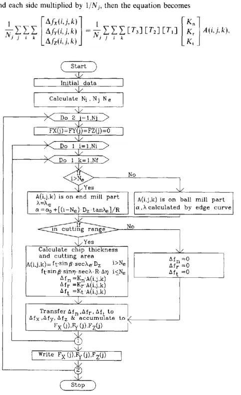
+ cvf 3 + csf2hd + c9fth 2 4- c,oh 3, (23) where c~-c,o are constant parameters that can be estimated by the regressive method from the values of Kn, Kr, and Kt obtained for different cutting conditions. These polynomial models provide a good fit to the specific cutting forces K,, Kr, and Kt, within the operating range of interest, the percentages of prediction errors of Kn, Kr, and Kt being less than 10%. Once parameters are obtained, the geometric parameters :~ and 2 are employed to calculate the instantaneous chip thickness, cutting area, and cutting force. A flow chart of the entire modeling procedure is given in Fig. 8.
5. Comparison between experimental and numerical results
5.1. Experimental set-up and conditions
The experimental set-up is shown in Fig. 9. The cutting forces were measured using a Kistler 9257B dynamometer and the data were collected by a data-acquisition system. The cutter used was a Nachi high-speed steel ball-end mill. Whilst the workpieces used were T6061, T2024, and T7075 aluminum alloy with hardness values of 55, 77 and 84 HRB (Hardness Rockwell B), respectively.
244 S.-T. Chiang et al. / Journal o/Materials Processing Technology 47 (1995) 231 249
+X +Y +Z
Limit switch Transformer Pulse
(--;.(/Aoptieal I
I ) Y / I c°up ler t - - ~ ~ [ F ~ I / ~ / linterface / x I ~ / ~ ' ~ " I ~ 1 / P o s i t i o n loop/ ihlYhl//control
// ] Z X i Linear scale // / r Data
Z ,' ~, / acquisition Yc~X c:~ Amplifier ~ l [ l Proximity / [ Cutter ~ IEEE488 Charge [ Xy Ampliiier~r___ j I Z X Y I Z [ [ Dynamometer O 0 Digital ~I oscilloscope Nicolet 2090 Fig. 9. Experimental set-up.The experiments consisted of two parts: one part was designed to determine the specific cutting forces and, thus, to obtain the cutting force model; the other part was used to verify the cutting force when the process contains the end-mill part of ball end milling. The cutting conditions for these two parts are listed in Table 2.
5.2. Experimental results and discussion
5.2.1. The relationship between K , , Kr, Kt andJ~, hd
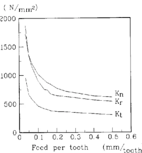
The experiments performed to determine K,, Kr, and Kt were conducted with 180 cutting conditions from the combination of the conditions listed in Table 2. Thus, 180 values of K,, Kr, and K, were obtained from Eq. (22). Fig. 10 presents the values obtained for K,, Kr, and K, vs. feed per toothft for the workpiece of hardness 84 HRB. From this figure, It is seen that Kn, Kr, and K, decrease as the feed per tooth increases. It is also noted that the specific cutting force Kt is minimum and the specific cutting force K, is maximum, amongst the values of Kn, Kr, and K,.
S.-T. Chiang et al. / Journal of Materials Processing Technology 47 (1995) 231 249 Table 2
The cutting conditions
245 Experiments (part 1) Cutting conditions Experiments (part 2) Cutting conditions Down milling, 6 A~ = 0 Spindle speed: 300, 600, 900 rpm Feedrate: 1, 2, 3, 4, 5 mm/s Hardness: 55, 77, 84 HRB Axial dept of cut: 3, 6 mm Radial depth of cut: 4, 8 mm No coolant
Down milling, 6A~ = 0 Spindle speed: 900 rpm Feedrate: 1, 2, 3 mm/s Hardness: 55, 77, 84 HRB Axial depth of cut: 12, 16 mm Radial depth of cut: 1, 2, 3 mm No coolant Table 3 Coefficients of K , K and K~ K K Kq ¢'j - 1 . 1 4 0 x l 0 , 3 1 . 8 0 0 x 1 0 3 - 5 . 1 0 0 x 1 0 -4 ¢'2 - 1.685 x 10⁴ - 2.850 x 10⁴ - 1.053 x 10⁴ c 3 1.087 x 10² 1.507 x 10² 7.204 x 101 ¢'4 1.399 x 10⁴ 2.059 × 10⁴ 7.189 x 10³ c s 3.977 × 10: 7.069 × 10² 2.669 x 10² ¢'6 - 2.590 x 10 ° 4.030 x 10 ° - 1.958 x 10 ° c~ -- 2.955 × 10⁴ - 4.292 x ]04 - 1.667 x 10'* c s 2.023 × 10² 2.861 x 10² 1.219 x 10² % -- 3.902 x 10 ° - 6.552 x 10 ° - 2.535 x 10 ° clO 1.885 x 10 ,2 3.059 x 10 -2 1.467 x 10 -2 F i g . l 0 a l s o s h o w s t h e r e l a t i o n s h i p b e t w e e n K n , K r , a n d K t w h e n )'i > 0 . 2 ( r a m / t o o t h ) , K r ~ 0 . 8 8 K , , K t ~ 0 . 5 0 K , . (24) T h i s r e l a t i o n s h i p c o n f i r m i n g t h e a s s u m p t i o n in [ 1 , 2 ] t h a t t h e r e is a l i n e a r r e l a t i o n s h i p b e t w e e n K , , K r , a n d K , . H o w e v e r , w h e n f , < 0.2 ( m m / t o o t h ) t h i s a s s u m p t i o n is n o t c o r r e c t . T h i s e r r o r is a v o i d e d i n t h e p r e s e n t p a p e r , b e c a u s e K . , K r , a n d K t h a v e b e e n c o n s i d e r e d i n d e p e n d e n t l y o f e a c h o t h e r .
5.2.2. Comparison between experimental and simulation results.[or the ball part A f t e r t h e s p e c i f i c c u t t i n g f o r c e s a r e o b t a i n e d , t h e c u t t i n g f o r c e c a n b e p r e d i c t e d b y i n s e r t i n g t h e s e v a l u e s i n t o t h e c u t t i n g f o r c e m o d e l . S o m e o f t h e p r e d i c t e d a n d
246 S.-T. Chiang et al. / Journal ~?f Materials Processing Technology 47 (1995) 231 249 ( N / r a m 2) 2000 1500 1000 500
I,
Kn Kr Kt I , I , I , I , I , 0.1 0.2 0.3 0.4 0.5 0.6Feed per t o o t h -'~.(mm/'oot~)
Fig. 10. The specific cutting force K., Kr, K, vs. feed per tooth for the workpiece of hardness HRB = 84.
Table 4
Actual and predicted cutting-forces of the part 1 experiments (radial depth of cut R d = 4 mm) No .[i h d A d rpm Measured forces (N) Predicted forces (N)
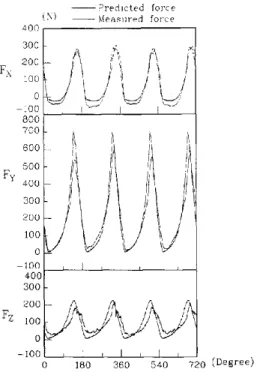
(mm/ (HRB) (mm) tooth) F x Fy F z F x Fy F z 1 0.033 55 3 900 18.6 62.6 42.2 15.4 60.1 35.6 2 0.033 77 3 900 17.2 80.5 58.1 16.1 77.7 50.8 3 0.033 84 3 900 24.1 116.6 101.3 19.1 102.6 77.9 4 0.050 55 6 600 24.3 78.8 49.7 22.0 82.1 46.4 5 0.050 77 6 600 24.9 102.0 62.2 22.3 104.9 65.8 6 0.050 84 6 600 31.4 140.6 108.3 26.5 139.6 103.9 7 0.067 55 3 900 16.1 61.9 45.4 16.9 58.1 43.8 8 0.067 77 3 900 16.9 76. I 60.5 17.3 72.1 60.9 9 0.067 84 3 900 17.5 102.3 96.7 22.5 94.3 95.9 10 0.100 55 6 600 20.7 74.3 58.7 23.3 76.0 52.1 11 0.100 77 6 600 16.7 95.0 73.4 22.4 90.7 69.8 12 0.100 84 6 600 19.5 124.7 112.9 29.1 119.1 115.5 13 0.200 55 3 300 47.8 101.6 61.9 42.1 125.2 75.6 14 0.200 77 3 300 31.5 156.4 105.0 34.0 129.4 80.2 15 0.200 84 3 300 31.1 184.5 153.8 42.5 160.7 135.8 16 0.200 55 6 300 69.6 202.5 89.8 70.8 213.0 100.0 17 0.200 77 6 300 75.7 250.4 122.8 69.9 201.0 96.2 18 0.200 84 6 300 85.4 281.9 189.5 82.9 243.9 161.4 e x p e r i m e n t a l c u t t i n g f o r c e s f o r t h e s a m e c u t t i n g c o n d i t i o n s a r e l i s t e d in T a b l e 4, a n d o n e o f t h e c a s e s is s h o w n in Fig. 11. I n t h i s l a t t e r f i g u r e , t h e t r e n d in t h e m e a s u r e d a n d p r e d i c t e d f o r c e s is s i m i l a r in e v e r y r e s p e c t . T h e r e s u l t s in t h e t a b l e s h o w a l s o t h a t t h e m e a n f o r c e e r r o r s a r e less t h a n 1 5 % a n d a r e t h u s m o r e a c c u r a t e t h a n t h e e r r o r o f 2 0 % g i v e n in [ 5 ] , w h i c h is b e c a u s e in t h e p r e s e n t w o r k t h e c u t t i n g r a n g e is c o n s i d e r e d m o r e
S.-T. Chiang et al. / Journal 0[" Materials Processing Technology 47 (1995) 231 249 247 Fx (Y) 40O 30O 20O 100 0 -3.00 8OO 7 0 0 60O 50O ~y 4OO 3(?0 2O0 100 0 100 4OO - - P r e d i c t e d force - - M e a s u r e d forc:e
/
/
.,,
Fz 300 F I 10 -I00 [ I r I I ~ I 0 180 3 6 0 5 4 0 7 2 0 ( D e g r e e )Fig. 11. Comparisons of predicted and actual cutting-forces in the X, Y, and Z directions. (test number 16 of Table 4 with v = 300 rpm, h~ = 55 HRB, Ad = 6 mm, Ra = 4 mm, ft = 0.2 mm/tooth).
adequately and a more accurate force model is used. The remaining predictive errors can be attributed to the following:
1. Although the assumption that K,, K,, and Kt are a third-order function o f f and h~ is reasonable, a small error still exists.
2. The deflection of the cutter is neglected.
3. There is an error between the actual profile of the edge and the approximate profile. Because of reason 2, as shown in Fig. 11, the predicted value of the Y direction force at the apogee is greater than the experimental value, since the deflection makes the real radial depth of cut less than the given depth of cut.
5.2.3. Comparison between experimental and simulation results ,for both the ball and end-mill parts
Selected results on the cutting force for both the ball and the end-mill parts from simulation and experiment are listed in Table 5, and one particular case is shown in Fig. 12. The results show that the error is less than 20%, which is slightly greater than the error described in Section 5.2.2. The error is greater because the rake angle was derived using the model of the ball-end-mill part, which has a bias to the real rake angle of the end-mill part. Thus, the derived coefficients cl-c~o in the specific cutting forces generate an error, which error can be decreased by considering these coeffi- cients separately for the ball part and the end-mill part.
248 S.-T. Chiang et al. / Journal o f Materials Processing Technology 47 (1995) 231-249
Table 5
Actual and predicted cutting-forces of the part 2 experiments (radial depth of cut R d = 2 m m and spindle speed v = 900 rpm)
No f h d A d Measured forces (N) Predicted forces (N)
(mm/ (HRB) (ram) tooth) F x F r F z F x F r F z 1 0.033 55 12 35.9 62.8 27.9 27.7 52.4 17.2 2 0.033 77 12 39.3 72.4 28.6 32.0 72.0 25.3 3 0.033 84 12 45.5 114.7 57.1 39.4 98.0 41.8 4 0.067 55 12 58.0 94.5 37.8 48.9 88.5 24.9 5 0.067 77 12 60.4 102.7 40.0 54.2 114.8 36.3 6 0.067 84 12 67.8 147.5 70.8 66.7 159.8 65.2 7 0.033 55 16 50.2 84.9 26.9 94.8 70.3 14.6 8 0.033 77 16 50.0 86.3 27.8 40.0 93.7 22.3 9 0.033 84 16 52.6 127.4 51.8 48.8 128.6 30.3 10 0.067 55 16 75.1 114.4 31.8 61.6 114.3 19.9 11 0.067 77 16 76.4 123.7 33.9 67.9 148.9 30.4 12 0.067 84 16 83.2 167.7 59.7 82.8 209.3 60.6 - - P r e d i c t e d force (N) - - Measured force 200 ] Fx lO!5 250 200 150 Fy lOO 5O 0 - 5 0 ~ I ~ I ~ I lO0 Fz o - 5 0 ~ I ~ I L I 0 180 360 540 720 (Degree)
Fig. 12. C o m p a r i s o n s of predicted and actual cutting forces in X, Y, and Z directions. (test n u m b e r 1 of Table 5 with v = 900 rpm, hd = 55 HRB, Ad = 12 ram, Rd = 2 ram, f, = 0.033 ram/tooth).
6. Conclusions
T h i s p a p e r d e v e l o p s a m e t h o d f o r p r e d i c t i n g t h e c u t t i n g f o r c e i n b a l l - e n d m i l l i n g . T h e m e t h o d is s i m p l e a n d y i e l d s a m o r e a c c u r a t e c u t t i n g - f o r c e m o d e l , a t t r i b u t e d t o t h e f o l l o w i n g : (i) a c o r r e c t d e s c r i p t i o n o f t h e c u t t i n g e d g e ; (ii) c o m p l e t e c u t t i n g
S.-T. Chiang et al. / Journal ~['Materials Processing Technology 47 (1995) 231 249 249 boundary conditions; and (iii) an adequate transformation of the infinitesimal cutting force.
The results of the simulations and experiments reported here support the following conclusions:
1. If the axial depth of cut is greater than the radius of the cutter, the cutting force can still be predicted using the proposed cutting-force model.
2. In the proposed method, the slope of the edge is approximated in the end mill part by the angle 2e instead of the saw-tooth approximation. Using the angle ,;~ results in far less bias of profile fitting and thus in a much lesser prediction error. 3. The appropriate range of entry angle/~en due to the cusp effect is considered in this
paper and a more accurate cutting range is given, i.e., the cutting force is estimated much more accurately.
References
[1] J. Tlusty and P. Macneil, Dynamics of cutting forces in end milling, Ann. CIRP 24, (1975), 20 25. [2] W.A. Kline, R.E. Devor and J.R. Lingberg, The prediction of cutting forces in end milling with
application to cornering cuts, Int. J. Math. Tool Des. Res., 22(1) (1982) 7 22.
[3] W.A. Kline and R.E. Devor, The effect of runout of cutting geometry and forces in end milling, Int. J. Math. Tool Des. Res., 23(2/3) (1983) 123 140.
[4] Y. Fujii and T. Terai, Ball-nose end mills simulator Simulation of a cutting force, J. Japan Soc. Prec'. Eng. (in Japanese), 54(12) (1988) 2301 2306.
[5] M. Yang and H.D. Park, The prediction of cutting forces in ball end milling, Int. J. Math. Tool Manufl, 31(1) (1991) 45-54.
[6] A. Hirota and E. Usui, Analytical prediction of cutting forces in slab milling operation, Bull. Japan Soc. Prec'. En9., 15(1) (1981) 40-46.